Fixed Points Structure & Effective Fractional Dimension
for $O(N)$ Models with Long–Range Interactions

Abstract

We study $O(N)$ models with power–law interactions by renormalization group (RG) methods: when the wave function renormalization is not present or not field dependent, their critical exponents can be computed from the ones of the corresponding short–range $O(N)$ models at an effective fractional dimension. Explicit results in $2$ and $3$ dimensions are given for the exponent $\nu$. We propose an improved RG to describe the full theory space of the models where both short–range and long–range interactions are present and competing, and no a priori choice among the two in the RG flow is done: the eigenvalue spectrum of the full theory for all possible fixed points is drawn and the effective dimension shown to be only approximate. A full description of the fixed points structure is given, including multicritical long–range universality classes.

$O(N)$ models are celebrated and tireless workhorses of statistical mechanics and play a key role in the field of critical phenomena: from one side the interest for their properties motivated the developments of numerous - analytical and numerical - techniques, from the other side they are concretely used as a test ground to benchmark the validity of new techniques for critical phenomena and lattice models.

Among the interactions studied in the context of $O(N)$ models an important and paradigmatic role is played by long–range (LR) interactions, having the form of power–law decaying couplings. A first reason is that the results can be contrasted with the findings obtained for short–range (SR) interactions, to explore how universal and non–universal quantities change increasing the range of the interactions. Apart from this motivation per se, internal to $O(N)$ models, another even more important reason for such studies is given by the long–lasting interest in understanding the properties of systems with LR interactions motivated by their crucial presence in many systems ranging from plasma physics to astrophysics and cosmology Dauxois10 . For a general $O(N)$ model with power–law interactions the Hamiltonian reads

$$H=-\frac{J}{2}\sum_{i\neq j}\frac{\mathbf{S}_{i}\cdot\mathbf{S}_{j}}{|i-j|^{d+\sigma}}\,,$$ (1)

where $\mathbf{S}_{i}$ denote a unit vector with $N$ components in the site $i$ of a lattice in dimension $d$, $J$ is a coupling energy and $d+\sigma$ is the exponent of the power–law decay (we refer in the following to cubic lattices). When $\sigma\leq 0$ a diverging energy density is obtained and to well define the thermodynamic limit it is necessary to rescale the coupling constant $J$ Campa09 . When $\sigma>0$ the model may have a phase transition of the second order, in particular as a function of the parameter $\sigma$ three different regimes occur Fisher72 ; Sak73 : (i) for $\sigma\leq d/2$ the mean–field approximation is valid even at the critical point; (ii) for $\sigma$ greater than a critical value, $\sigma_{*}$, the model has the same critical behaviour of the SR model (formally, the SR model is obtained in the limit $\sigma\to\infty$); (iii) for $d/2<\sigma\leq\sigma_{*}$ the system exhibits peculiar LR critical exponents. For the Ising model in $d=1$ Dyson69 ; Thouless69 ; Anderson70 the value $\sigma_{*}=1$ is found, and for $\sigma=\sigma_{*}$ a phase transition of the Berezinskii-Kosterlitz-Thouless universality class occur Cardy81 ; Froelich82 ; Luijten01 (see more references in Luijten97 ). Many efforts have been devoted to the determination of $\sigma_{*}$ and to the characterization of the universality classes in the region $d/2<\sigma\leq\sigma_{*}$ for general $N$ in dimension $d\geq 2$, which is the case we are going to consider in this paper. In the classical paper Fisher72 the expression $\eta=2-\sigma$ was found for the critical exponent $\eta$ by an $\epsilon$-expansion (at order $\epsilon^{2}$) and conjectured to be exact, implying a discontinuity in $\sigma_{*}$, where $\sigma_{*}=2$ Fisher72 .
A way out was proposed by Sak Sak73 , who found $\eta=2-\sigma$ for all $\sigma<\sigma_{*}$ and gave $\sigma_{*}=2-\eta_{SR}$ (where $\eta_{SR}$ is the $\eta$ exponent of the SR model). This $\eta$ is a continuous function of $\sigma$ and there is no correction to the canonical dimension of the field in the case of LR interactions. Subsequent Monte Carlo (MC) results, based on MC algorithms specific for LR interactions Luijten95 , confirmed this picture Luijten02 . However the Sak scenario was recently challenged by new MC results Picco12 , suggesting that the behavior of the anomalous dimension may be far more complicated that the one provided by Sak Sak73 . Defining the critical exponent $\eta_{LR}$ of the $O(N)$ LR models in dimension $d$ with power–law exponent $d+\sigma$ as

$$\eta_{LR}(d,\sigma)\equiv 2-\sigma+\delta\eta\,,$$ (2)

in Picco12 it was reported that there is a non–vanishing correction $\delta\eta$ to Sak’s result $\eta=2-\sigma$ in the region $d/2<\sigma<\sigma_{*}$ and that $\sigma_{*}=2$, as in the earliest work of Fisher, Ma and Nickel Fisher72 . In a subsequent work Blanchard13 the presence of a $\delta\eta\neq 0$ was discussed using an $\epsilon$–expansion, and as a result the correction $\delta\eta$ should be less than the anomalous dimension of a SR system in dimension $D_{\rm eff}^{BPR}\equiv 4+d-2\sigma$ (we refer to such dimension as $D_{\rm eff}^{BPR}$ from the authors of Blanchard13 ). In the following we are going to show that most of the critical properties of a LR model in dimension $d$ with power law exponent $d+\sigma$ can be inferred from those of a SR model in the effective fractional dimension $D_{\rm eff}=2d/\sigma\neq D_{\rm eff}^{BPR}$, this result being exact in the $N\to\infty$ limit. We also observe that the MC results recently presented for a percolation model with LR probabilities Grassberger13 seem to agree with the findings of Picco12 and not with the Sak scenario. In a very recent work new MC results for the Ising model with LR interaction in $d=2$ were presented Parisi14 : these results evidence the presence of logarithmic corrections into the correlation function of this kind of systems when the value of $\sigma$ is very close to $\sigma=2-\eta_{SR}$, implying the numerical difficulty of extracting reliable results for the critical exponents with small error bars around $\sigma=2-\eta_{SR}$.

The controversy about the actual value of $\sigma_{*}$ raised by recent MC results has not really a compelling quantitative raison d’être: after all, for the Ising model in $d=2$ it is $\eta_{SR}=1/4$ and $\sigma_{*}=7/4$ predicted by Sak should be contrasted with $\sigma_{*}=2$ suggested in Picco12 (even though the value of $\eta$ at $\sigma=7/4$ obtained in Picco12 is $\eta=0.332$ and it should be contrasted with $\eta=1/4$ predicted by Sak). The issue raised by recent MC results is rather of principle, since it generally questions how the LR terms ($p^{\sigma}$) renormalize and especially how the SR term ($p^{2}$) in the propagator is dressed by the presence of LR interactions. In this paper we aim at clarifying such issues using a functional renormalization group approach Berges02 ; Delamotte07 .

We are interested in universal quantities, and as usual we replace the spin variables $\{\mathbf{S}_{i}\}$ with an $N$–component vector field $\boldsymbol{\phi}(x)$ in continuous space. We define a scale dependent effective action $\Gamma_{k}$ depending on an infrared cutoff $k$ and on the continuous field $\boldsymbol{\phi}$: when $k\rightarrow k_{0}$, where $k_{0}$ is some ultraviolet scale, the effective action is equal to the mean–field free energy of the system, while for $k\rightarrow 0$ it is equal to the exact free energy Berges02 . Our first ansatz for the effective action reads

$$\Gamma_{k}[\phi]=\int d^{d}x\left\{Z_{k}\partial^{\frac{\sigma}{2}}_{\mu}\phi_{i}\partial^{\frac{\sigma}{2}}_{\mu}\phi_{i}+U_{k}(\rho)\right\}\,,$$ (3)

where the summation over repeated indexes is assumed, $\rho=\frac{1}{2}\phi_{i}\phi_{i}$, and $\phi_{i}$ is the $i$–th component of $\boldsymbol{\phi}$. The notation $\partial^{\frac{\sigma}{2}}_{\mu}$ is a compact way to intend that the inverse propagator of the effective action (3) in Fourier space depends on $q^{\sigma}$ and not on $q^{2}$ as in the SR case. $Z_{k}$ is the wave function renormalization of the model that at this level of approximation is field independent. The effective potential $U_{k}(\rho)$ satisfies a renormalization group equation Wetterich93 ; when this is rewritten in terms of dimensionless variables (denoted by bars) one can find the fixed points, or scaling solutions, $\bar{U}_{*}(\bar{\rho})$ by solving it Codello12 . Using an infrared cutoff suited for LR interactions, $R_{k}(q)=Z_{k}(k^{\sigma}-q^{\sigma})\theta(k^{\sigma}-q^{\sigma})$, we obtain the flow equation for the effective potential,

$$\begin{split}&\partial_{t}\bar{U}_{k}=-d\bar{U}_{k}(\bar{\rho})+(d-\sigma+\delta\eta)\bar{\rho}\,\bar{U}^{\prime}_{k}(\bar{\rho})\\ &+\frac{\sigma}{2}c_{d}(N-1)\frac{1-\frac{\delta\eta}{d+\sigma}}{1+\bar{U}^{\prime}_{k}(\bar{\rho})}+\frac{\sigma}{2}c_{d}\frac{1-\frac{\delta\eta}{d+\sigma}}{1+\bar{U}^{\prime}_{k}(\bar{\rho})+2\bar{\rho}\,\bar{U}^{\prime\prime}_{k}(\bar{\rho})}\,,\end{split}$$ (4)

where $c_{d}^{-1}=(4\pi)^{d/2}\Gamma\left(d/2+1\right)$ and $\delta\eta$ is an eventual anomalous dimension correction, related to the flow of the wave function renormalization by $\delta\eta=-\partial_{t}\log Z_{k}$, where $t=\log(k/k_{0})$ is the RG time and $k_{0}$ is the ultraviolet scale.

We start our analysis considering the case $Z_{k}=1$, which implies $\delta\eta=0$. It is then possible to show that the flow equation (4) for the effective potential can be put in relation with the corresponding equation for a SR model Codello12 ; Morris94 in an effective fractional dimension

$$D_{\rm eff}=\frac{2d}{\sigma}$$ (5)

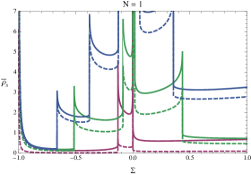
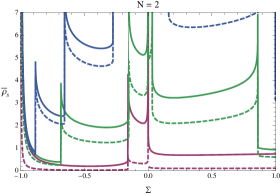
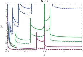
(in the following we denote by capital $D$ the dimension of the SR $O(N)$ model). Namely, we can see that the LR and SR universality classes in, respectively, dimension $d$ and $D_{\rm eff}$ are the same at this level of approximation. The equivalence between the fixed point structure of these two models can also be seen using the spike plot technique described in Codello12 ; Morris94 : the corresponding figure may be found in the Appendix A.

From this analysis it follows that by varying $\sigma$ at fixed $d$ we go trough a sequence of $\sigma_{c,i}$ at which new multicritical LR universality classes appear, in a way analogous to the sequence of upper critical dimensions found in SR models as $d$ is varied Codello12 . For the Ising universality class the lower critical decay exponent is $\sigma_{c,2}=d/2$ in agreement with known results Fisher72 . In the case of a $i$–th multicritical model with LR interaction the lower critical decay exponent is found to be $\sigma_{c,i}=\frac{d(i-1)}{i}$. Since the new fixed points branch from the Gaussian fixed point, their analysis based on the ansatz (3), first term of an expansion of the effective action in powers of the anomalous dimension, is consistent and the existence of multicritical LR $O(N)$ models can be extrapolated to be valid in the full theory.

Within this approximation it is also possible to establish a mapping between the LR correlation length exponent $\nu_{LR}(d,\sigma)$ and the equivalent SR one $\nu_{SR}(D_{\rm eff})$. The relation is found to be:

$$\nu_{LR}(d,\sigma)=\frac{2}{\sigma}\nu_{SR}(D_{\rm eff})\,.$$ (6)

As a check, we observe that relations (5) and (6) are satisfied exactly by the spherical model Joyce . In fact in the $N\to\infty$ limit our approximation provides exact critical exponents Tetradis94 .

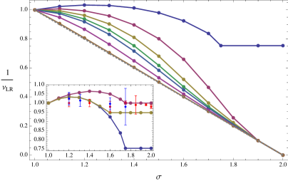
Figure 1: $y_{t}=1/\nu_{LR}$ exponent as a function of $\sigma$ in $d=2$ for some values of $N$ (from top: $N=1,2,3,4,5,10,100$). The dashed line is the analytical result obtained for the spherical model $N=\infty$. Inset: $y_{t}=1/\nu_{LR}$ vs. $\sigma$ for the $d=2$ LR Ising model compred with MC data of Luijten02 (red circles) and of Parisi14 (blue circles). The three continuous lines represents the estimates made using (8) with the numerical values of $\nu_{SR}(D_{\rm eff}^{\prime})$ and $\eta_{SR}(D_{\rm eff}^{\prime})$ taken from recent high–precision estimates in fractal dimensions El14 (top red line), from Codello13 ; Codello14 where the $O(N)$ model definition for $\eta_{SR}$ is used (blue bottom line) and from Codello12 where the Ising definition of $\eta_{SR}$ is used instead (yellow middle line) El14 .

To study anomalous dimension effects one has to study the equation for the effective potential $U_{k}$ in the case $\delta\eta\neq 0$, i.e. when $Z_{k}$ in (3) is non–constant. One obtains the scale derivative of the wave function renormalization from $\partial_{t}Z_{k}=\lim_{p\rightarrow 0}\frac{d}{dp^{\sigma}}\partial_{t}\Gamma_{k}^{(2)}(p,-p)$ and computes the anomalous dimension using $\delta\eta=-\partial_{t}\log Z_{k}$. Since the flow equation generates no non–analytic terms in $p$, from this definition we find $\delta\eta=0$, in agreement with Sak’s result Sak73 , in which the anomalous dimension does not get any non mean–field contribution. However, an anomalous dimension is present, at this approximation level, in the SR system, thus we obtain a new dimensional equivalence:

$$D_{\rm eff}^{\prime}=\frac{[2-\eta_{SR}(D_{\rm eff}^{\prime})]d}{\sigma}\,,$$ (7)

which is in agreement with the results of the dimensional analysis performed for the Ising model in Parisi14 and with the arguments presented for the LR and SR Ising spin glasses in Young12 . Eq. (7) is valid for any $N$ and it is an implicit equation for $D_{\rm eff}^{\prime}$: to find $D_{\rm eff}^{\prime}$ one has to know the critical exponent $\eta_{SR}$ in fractional dimension Codello13 ; Katz77 ; Holovatch93 ; El14 . At date the most precise evaluation of $\eta_{SR}$ for the Ising model ($N=1$) in fractional dimension is given in El14 ; results for general $N$ are given by in Codello13 , turning in rather good agreement with El14 for $N=1$ and with Holovatch93 for $N\geq 2$.

In the case of a running, not field dependent, wave function renormalzation we also obtain the following relation for the critical exponent $\nu_{LR}$:

$$\nu_{LR}(d,\sigma)=\frac{2-\eta_{SR}(D_{\rm eff}^{\prime})}{\sigma}\,\nu_{SR}(D_{\rm eff}^{\prime})\,.\\$$ (8)

In Fig. 1 we compare the exact behaviour for the $y_{t}=1/\nu_{LR}$ LR exponent in the spherical $N\to\infty$ limit with the behaviour obtained using the effective dimension $D^{\prime}_{eff}$ for various values of $N$. In the inset of Fig.  1 we plot MC results from Luijten02 and Parisi14 together with the results obtained by the effective dimension $D_{\rm eff}^{\prime}$ both at our approximation level and with the use of high–precision estimates of the SR critical exponents in fractal dimensions from El14 in (7). We expect these results to be more reliable as $N$ grows due to the relative decrease of anomalous dimensions effects in these cases. Relations (7) and (8) can be also used to extend this analysis to multicritical fixed points in LR systems. We also note the fact that in $d=2$ for every $N\geq 2$ the exponent $y_{t}$ goes to zero, and thus $\nu_{LR}$ goes to infinity, is a consequence of, and consistent with, the Mermin–Wagner theorem Codello13 .

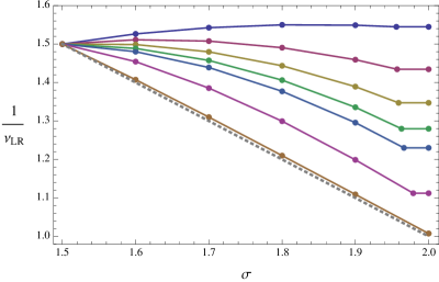
In Fig. 2 we plot the exponent $y_{t}$ for various $N$ in three dimensions using (7): due to the better performances of our approximation in three dimensions, we expect these results to be quantitatively very reliable, when compared with future numerical simulations. The curves of Fig. 1 and Fig. 2 are genuine universal predictions of our analysis and to our knowledge are new.

Figure 2: $y_{t}=1/\nu_{LR}$ exponent as a function of $\sigma$ in $d=3$ for some values of $N$ (from top: $N=1,2,3,4,5,10,100$). As in Fig. 1 the dashed line is the analytical result obtained for the spherical model.

The present analysis suggests the validity of Sak’s results for the value of $\sigma_{*}$. On the other hand, since the ansatz (3) does not contain any SR term, such approximation is not able to describe the case $\sigma>\sigma_{*}$, in which SR interactions could become dominant. In order to investigate these effects we enlarge our theory space and we propose the new ansatz:

$$\Gamma_{k}[\phi]=\!\int\!d^{d}x\!\left\{\!Z_{\sigma,k}\partial^{\frac{\sigma}{2}}_{\mu}\phi_{i}\partial^{\frac{\sigma}{2}}_{\mu}\phi_{i}\!+\!Z_{2,k}\partial_{\mu}\phi_{i}\partial_{\mu}\phi_{i}\!+\!U_{k}(\rho)\!\right\}\,,$$ (9)

where we have both LR and SR terms in the propagator. A similar ansatz was introduced in Tissier14 ; Balog14 where the dimensional reduction of the Ising model with LR interaction in presence of disorder was studied.

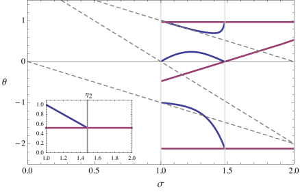
Figure 3: Eigenvalues ($\theta$) of the RG stability matrix in $d=2$ as a function of $\sigma$ for the SR (red lines) and LR (blue lines) fixed points. Mean field exponent are represented by dashed lines. The vertical lines mark $\sigma=\frac{d}{2}=1$ and $\sigma_{*}=2-\eta_{SR}$. For $1<\sigma<\sigma_{*}$ both fixed points are present, but the LR one has two IR attractive directions, while the SR has one. For $\sigma>\sigma_{*}$ only the SR fixed point is present, while for $\sigma<1$ the LR fixed point is Gaussian and the exponent are mean field. Inset: anomalous dimension $\eta_{2}$ vs. $\sigma$ in the same case.

We need to choose a proper cutoff function for the propagator of the theory (9). Since we do not know a priori which will be the dominant term for $\sigma\simeq\sigma^{*}$ we take the following combination:

$$R_{k}(q)=Z_{\sigma,k}(k^{\sigma}-q^{\sigma})\theta(k^{\sigma}-q^{\sigma})+Z_{2,k}(k^{2}-q^{2})\theta(k^{2}-q^{2})\,.$$ (10)

The ansatz (9) and the cutoff choice (10) are consistent with the ones of the previous analysis when LR interactions are dominant, but they are still valid when SR become important and will allow us to study the whole $\sigma$ range. The general flow equations that follows and further details are reported in the Appendix B.

To further proceed, we make a Taylor expansion of the effective potential around its minimum and we maintain only the lowest terms: $\bar{U}_{k}(\bar{\rho})=\frac{1}{2}\lambda_{k}(\bar{\rho}-\kappa_{k})^{2}$. In addition to the equations for $\lambda_{k}$ and $\kappa_{k}$ we have also an equation for the anomalous dimension $\eta_{2}=-\partial_{t}\log Z_{2,k}$ and one for the LR coupling $J_{\sigma,k}\equiv Z_{\sigma,k}/Z_{2,k}$. Here we report these equations in the two dimensional $N=1$ case:

$$\eta_{2} = \frac{(2+\sigma\bar{J}_{\sigma,k})^{2}\kappa_{k}\lambda_{k}^{2}}{(1+\bar{J}_{\sigma,k})^{2}(1+\bar{J}_{\sigma,k}+2\kappa_{k}\lambda_{k})^{2}}$$

$$\partial_{t}\kappa_{k} = \;-\eta_{2}\kappa_{k}+3\frac{1-\frac{\eta_{2}}{d+2}+\frac{\sigma}{2}\bar{J}_{\sigma,k}}{(1+\bar{J}_{\sigma,k}+2\kappa_{k}\lambda_{k})^{2}}$$

$$\partial_{t}\lambda_{k} = 2(-1+\eta_{2})\lambda_{k}+18\lambda_{k}\frac{1-\frac{\eta_{2}}{d+2}+\frac{\sigma}{2}\bar{J}_{\sigma,k}}{(1+\bar{J}_{\sigma,k}+2\kappa_{k}\lambda_{k})^{3}}$$

$$\partial_{t}\bar{J}_{\sigma,k} = (\sigma-2)\bar{J}_{\sigma,k}+\eta_{2}\bar{J}_{\sigma,k}\,.$$ (11)

Using these equations we are able to describe in detail the structure of the phase diagram. The anomalous dimension of LR $O(N)$ models is still $\eta=2-\sigma$, then for $\sigma>\sigma_{*}=2-\eta_{SR}$ the dimensionless coupling $\bar{J}_{\sigma,k}$ is always renormalized to zero, whatever initial conditions we choose and the system behaves as if only SR interactions were present. On the other hand when $\sigma<\sigma_{*}$ a new interacting LR fixed point branches from the SR one and is characterized by a finite value of $\bar{J}_{\sigma,*}$.

In Fig. 3 we show the critical exponents of both SR and LR fixed points obtained from the coupling set (11). The SR fixed point has just one repulsive direction for $\sigma>\sigma_{*}$ (the standard Wilson–Fisher one) and the LR fixed point does not exist at all. At $\sigma=\sigma_{*}$ the smallest attractive eigenvalue hits zero and the LR fixed point emerges from the SR fixed point. For $\sigma<\sigma_{*}$, the SR fixed points has two repulsive directions while the LR one has just one repulsive direction. Finally at $\sigma=\frac{d}{2}=1$ the LR fixed point becomes Gaussian and for all $\sigma<\frac{d}{2}=1$ the behavior is mean field.

From the analysis of Fig. 3 one clearly understands that the LR fixed point is attractive along the direction which connects it to the SR (Wilson–Fisher) fixed point, thus for $\sigma<\sigma_{*}$ the SR fixed point becomes repulsive in the $\bar{J}_{\sigma,k}$ direction and the LR fixed point controls the critical properties of the system. In the $\sigma\rightarrow\sigma_{*}$ limit the LR fixed point moves towards the SR one and finally merges with it at $\sigma=\sigma_{*}$. This structure for the phase diagram implies that the anomalous dimension is given (as show in the inset of Fig. 3) by the LR value $\eta_{2}=2-\sigma$ for $\sigma<2-\eta_{SR}$ and by the SR value $\eta_{2}=\eta_{SR}$ for $\sigma>2-\eta_{SR}$, thus confirming Sak’s scenario. It is important to stress that we are not imposing this picture by hand, but it emerges dynamically form the solution of (11). It is also important to underline that the threshold $\sigma^{*}=2-\eta_{SR}$ is also generated dynamically, with the SR anomalous dimension appearing in it being the one pertinent to the approximation level considered.

Conclusions: We studied $O(N)$ long–range (LR) models in dimension $d\geq 2$. Using the flow equation for the effective potential alone we found that universality classes of $O(N)$ LR models are in correspondence with those of $O(N)$ short–range (SR) models in effective dimension $D_{\rm eff}=2d/\sigma$. We also found new multicritical potentials which are present, at fixed $d$, above certain critical values of the parameter $\sigma$.

We then considered anomalous dimension effects considering also the flow of a field independent wave function renormalization. Extending the approach described in Delamotte07 to the LR case we found $\delta\eta=0$, i.e. the Sak’s result Sak73 in which there are no correction to the mean–field value of the anomalous dimension. The relation between the LR model and the SR model is now valid at the effective dimension $D_{\rm eff}^{\prime}$ defined by Eq. (7), while the correlation length exponent is given according to Eq. (8). Quantitative predictions for the exponent $\nu_{LR}$ for various values of $N$ were as well presented in $d=2$ and $d=3$.

Finally we introduced an effective action where both the SR and LR terms are present. This approach does not impose a priori which is the dominant coupling in the RG flow. We showed how Sak’s result is again justified by the fixed point structure of the model, where a LR interacting fixed point appears only if $\sigma<\sigma_{*}$ and controls the critical behavior of the system. Interestingly, the effective dimension $D_{\rm eff}^{\prime}$ can be shown not to be exact at this approximation level: however it is possible to estimate the error committed using the effective dimension $D_{\rm eff}^{\prime}$, this error being proportional to the ratio between SR and LR couplings.

The final picture emerging from the our analysis is the following: starting at $\sigma=0$ and increasing $\sigma$ towards $2$ we have that for $\sigma<d/2$ only the LR Gaussian fixed point exists and no SR terms in the propagator are present. At $\sigma=d/2$ a new interacting fixed point emerges from the LR Gaussian one and the same happens at the values $\sigma_{c,i}$ where new LR universality classes appear (in the same way as the multicritical SR fixed points are generated below the upper critical dimensions). Finally, when $\sigma$ approaches $\sigma_{*}$ the LR Wilson–Fisher fixed point merges with its SR equivalent and the LR term in the propagator disappears for $\sigma>\sigma_{*}$: this has to be contrasted with the case $\sigma<\sigma_{*}$ where at the interacting LR fixed points the propagator contains also a SR term. The same scenario is valid for all multicritical fixed points, provided that the $\sigma_{*}$ values are computed with the corresponding SR anomalous dimensions.

Acknowledgements. We are very grateful to G. Gori and M.A. Rajabpour for many useful discussions during various stages of the work. We also acknowledge useful correspondence with I. Balog, G. Tarjus and M. Tissier. The CP³-Origins centre is partially funded by the Danish National Research Foundation, grant number DNRF90.

Note added: During the final phase of this work a paper on LR interactions appeared on the arXiv Parisi14_2 , showing that for $\sigma\simeq\sigma_{*}$ logarithmic corrections to the correlation function are present. We observe that the vanishing of the smallest attractive eigenvalues for the LR fixed point at $\sigma=\sigma_{*}$ shown in Fig.3 is in agreement with such finding.

Appendix A Pure long–range analysis

Let us consider a Ising model where the spins interacts via a long–range (LR) potential, with power low decaying interactions: the Hamiltonian reads

$$H=-\frac{J}{2}\sum_{i\neq j}\frac{\mathbf{S}_{i}\cdot\mathbf{S}_{j}}{|i-j|^{d+\sigma}}\,,$$ (12)

where $d$ is the dimension of the model and $d+\sigma$ the exponent of the power low decaying potential. We study the continuous field model analogous to the Hamiltonian (12). The effective action in the pure (LR) case reads:

$$\Gamma_{k}[\phi]=\int d^{d}x\left\{Z_{k}\partial^{\frac{\sigma}{2}}_{\mu}\phi_{i}\partial^{\frac{\sigma}{2}}_{\mu}\phi_{i}+U_{k}(\rho)\right\}\,,$$ (13)

where the summation over repeated indexes is assumed, $\rho=\frac{1}{2}\phi_{i}\phi_{i}$ and $\phi_{i}$ is the $i$–th component of $\boldsymbol{\phi}$. The notation $\partial^{\frac{\sigma}{2}}_{\mu}$ is a compact way to intend that the inverse propagator of the effective action (13) in Fourier space depends on $q^{\sigma}$. The effective potential $U_{k}(\rho)$ in (13) obeys the evolution equation derived in Wetterich93 . The evolution equation for the potential is as usual rewritten in terms of dimensionless variables,

$$\bar{U}_{k}(\bar{\rho}) =k^{-d}U_{k}(\rho)\,,$$ (14)

$$\bar{\rho} =Z_{k}k^{\sigma-d}\rho\,,$$ (15)

$$\bar{q} =k^{-1}q\,,$$ (16)

and then equated to zero, in order to find the fixed point solution $\bar{U}_{*}(\bar{\rho})$ Codello12 . We define a generalized Litim cutoff suited for long–range (LR) interactions:

$$R_{k}(q)=Z_{k}(k^{\sigma}-q^{\sigma})\theta(k^{\sigma}-q^{\sigma})\,.$$ (17)

Using (17) we obtain the equation:

$$\begin{split}\partial_{t}\bar{U}_{k}=&-d\bar{U}_{k}(\bar{\rho})+(d-\sigma+\delta\eta)\bar{\rho}\,\bar{U}^{\prime}_{k}(\bar{\rho})+\frac{\sigma}{2}c_{d}(N-1)\frac{1-\frac{\delta\eta}{d+\sigma}}{1+\bar{U}^{\prime}_{k}(\bar{\rho})}\\ &+\frac{\sigma}{2}c_{d}\frac{1-\frac{\delta\eta}{d+\sigma}}{1+\bar{U}^{\prime}_{k}(\bar{\rho})+2\bar{\rho}\,\bar{U}^{\prime\prime}_{k}(\bar{\rho})}\,,\end{split}$$ (18)

where $c_{d}^{-1}=(4\pi)^{d/2}\Gamma\left(d/2+1\right)$ and $\delta\eta$ is defined by

$$\delta\eta=-\frac{1}{Z_{k}}\partial_{t}Z_{k}\,,$$ (19)

is an eventual non–mean field correction to the anomalous dimension of the model, i.e. $\eta_{LR}\equiv 2-\sigma+\delta\eta$. Here $t=\log(k/k_{0})$ is the RG time.

Figure 4: Each value of $\Sigma\equiv\bar{U}_{*}^{\prime}(0)$ for which we have a spike in the above figure is the derivative at the origin of a well defined fixed point effective potential: thus every spike is the signature of a different universality class. Solid lines represents spike plots of LR models in dimension $d$ with power–law exponent $\sigma$, while dashed lines represent spike plots of SR models in dimension $D=D_{\rm eff}=2d/\sigma$. The plot is for the case $N=1,2,5$ and $d=2$ for the cases $\sigma=1.25,1.75,1.9$.

We first study the flow Eq. (18) in the case $Z_{k}=1$, i.e. we set $\delta\eta=0$. For comparison we report the analogous flow equation for the effective potential of the short–range (SR) model Delamotte07 :

$$\partial_{t}\bar{U}_{k}=-D\bar{U}_{k}(\bar{\rho})+(D-2+\eta_{SR})\bar{\rho}\,\bar{U}^{\prime}_{k}(\bar{\rho})+c_{D}(N-1)\frac{1-\frac{\eta_{SR}}{D+2}}{1+\bar{U}^{\prime}_{k}(\bar{\rho})}+c_{D}\frac{1-\frac{\eta_{SR}}{D+2}}{1+\bar{U}^{\prime}_{k}(\bar{\rho})+2\bar{\rho}\,\bar{U}^{\prime\prime}_{k}(\bar{\rho})}\,.$$ (20)

Here we denote by $D$ the dimension of the SR model, while $d$ is the dimension of the lattice in which the LR model is defined. The key point of our analysis is that if we make the substitution

$$D=D_{\rm eff}=\frac{2d}{\sigma}\,,$$ (21)

in (20) we obtain again Eq. (18) with $\delta\eta=0$, apart for a factor $\frac{\sigma}{2}$ multiplying the scale derivative of the potential. When we study the fixed point effective potential $\bar{U}_{*}(\bar{\rho})$ the scale derivative term in (18) vanishes and there is no difference between (18) and (20) with $D=D_{\rm eff}=2d/\sigma$, as it is shown in Fig. 1 of the main text.

We plot in Fig.4 the results obtained for three $O(N)$ models: $N=1$ (Ising model), $N=2$ (XY model) and $N=5$ (similar plots can be drawn for any $N$). From now on we reabsorb the coefficients $c_{d}$ and $c_{D}$ in the definition of the field, following the same procedure described in Morris94 . We now establish the mapping, valid within this approximation, between the LR correlation length exponent $\nu_{LR}(d,\sigma)$ and the equivalent SR one $\nu_{SR}(D_{\rm eff})$ at the effective dimension. This can be done following the procedure in Morris94 to evaluate these exponents. In order to calculate these exponents we have to write an eigenvalue equation for the stability of the perturbations around the scaling solution and then make the substitution

$$\bar{U}_{k}(\bar{\rho})=\bar{U}_{*}(\bar{\rho})+k^{y}\bar{u}_{k}(\bar{\rho})$$

in Eqs. (18) and (20). The $y$s are the renormalization group eigenvalues and the correlation length critical exponent is determined by the relation $\nu^{-1}=y_{t}=\min\{y\}$. The eigenvalue equations for the LR and SR perturbation $\bar{u}_{k}(\bar{\rho})$ are, respectively, the following:

$$(d-y_{LR})\bar{u}_{k}(\bar{\rho})-(d-\sigma)\bar{\rho}\,\bar{u}_{k}^{\prime}(\bar{\rho})+\frac{\sigma}{2}\frac{(N-1)\bar{u}_{k}^{\prime}(\bar{\rho})}{(1+\bar{U}^{\prime}_{*}(\bar{\rho}))^{2}}-\frac{\sigma}{2}\frac{\bar{u}_{k}^{\prime}(\bar{\rho})+2\bar{\rho}\,\bar{u}_{k}^{\prime\prime}(\bar{\rho})}{(1+\bar{U}^{\prime}_{*}(\bar{\rho})+2\bar{\rho}\,\bar{U}^{\prime\prime}_{*}(\bar{\rho}))^{2}}=0\,,$$ (22a)

and

$$(D-y_{SR})\bar{u}_{k}(\bar{\rho})-(D-2)\bar{\rho}\,\bar{u}_{k}^{\prime}(\bar{\rho})+\frac{(N-1)\bar{u}_{k}^{\prime}(\bar{\rho})}{(1+\bar{U}^{\prime}_{*}(\bar{\rho}))^{2}}-\frac{\bar{u}_{k}^{\prime}(\bar{\rho})+2\bar{\rho}\,\bar{u}_{k}^{\prime\prime}(\bar{\rho})}{(1+\bar{U}^{\prime}_{*}(\bar{\rho})+2\bar{\rho}\,\bar{U}^{\prime\prime}_{*}(\bar{\rho}))^{2}}=0\,,$$ (22b)

where $\bar{U}_{*}(\bar{\rho})$ is the scaling solution and the boundary condition is given in Morris94 . Evaluating the SR equation in dimension $D=D_{\rm eff}$ and multiplying both sides for $\sigma/2$ gives the result reported in the main text:

$$\nu_{LR}(d,\sigma)=\frac{2}{\sigma}\nu_{SR}(D_{\rm eff})\,.$$ (23)

Let us now consider the approximation in which the wavefunction renormalization $Z_{k}$ is running but field independent and study Eq. (18) in the case $\delta\eta\neq 0$. Defining $Z_{k}$ as

$$Z_{k}=\lim_{p\rightarrow 0}\frac{d}{dp^{\sigma}}\Gamma_{k}^{(2)}(p,-p)\,,$$ (24)

leads to the following result:

$$\delta\eta=0\,.$$

This is due to the peculiar properties of LR interactions, which lead to a non analytic term in the propagator. However when we calculate the RG time derivative of the propagator it does not present any non–analytic, at our approximation level, thus the flow leaves the $Z_{k}$ unaltered.

Thus in Eq. (18) we can just drop the $\delta\eta$ terms also in this case. Proceeding in the same way as done in the case $Z_{k}=1$ (performing an additional rescaling of the field), we obtain a new dimensional equivalence:

$$D_{\rm eff}^{\prime}=\frac{[2-\eta_{SR}(D_{\rm eff}^{\prime})]d}{\sigma}\,.$$ (25)

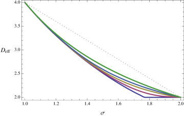
At date the most precise evaluation of $\eta_{SR}$ in fractional dimension $D$ for the Ising model ($N=1$) is given in El14 ; results for general $N$ are given in Codello13 , turning in rather good agreement with El14 for $N=1$ and with Holovatch93 for $N\geq 2$. Using these results we can then evaluate $D_{\rm eff}^{\prime}$ for various values of $N$ as shown in Fig. 5. The fact that the $N\geq 2$ curves reach two for $\sigma=2$ is due to the Mermin–Wagner theorem.

Figure 5: Different results for the effective dimension $D_{\rm eff}^{\prime}$ of a LR model $O(N)$ model in $d=2$:Ä (from left to right) $N=1,2,3,5,100$ using the data from Codello13 ; Codello14 . The $N=100$ case already overlaps with $D_{\rm eff}=2d/\sigma$ valid in the large–$N$ limit. The gray dashed line is the proposal made in Blanchard13 .

Following the previous procedure to compute the correlation length critical exponent now leads to the following relation:

$$\nu_{LR}(d,\sigma)=\frac{2-\eta_{SR}(D_{\rm eff}^{\prime})}{\sigma}\,\nu_{SR}(D_{\rm eff}^{\prime})\,.$$ (26)

The comparison of the exponent $y_{t}=1/\nu_{LR}$ for the LR Ising in $d=2$ obtained using (26) and Monte Carlo results from Luijten02 and Parisi14 is plotted in the inset of the Fig. 2 of the main text. Here we report other useful comment: the agreement is rather good for $\sigma\lesssim 1.75$, while for $\sigma\gtrsim 1.75$ the agreement becomes worst: this is due to the fact that in the SR case at this approximation level $\eta_{SR}(D=2)=0.233$ and then according to Sak one would have $\sigma_{*}=1.767$ which is not the exact value $\frac{7}{4}$ provided by Sak. Therefore, even if the result $\delta\eta=0$ is in agreement with Sak73 our prediction for $\nu_{LR}$ (blue line) has its own error due to the approximation of field independent wavefunction renormalization (e.g., the value of $\nu_{SR}(d=2)=1.05$, is not the exact one $\nu_{SR}(d=2)=1$). This is confirmed from the fact that using the numerically exact values of $\eta_{SR}$ in the equation (26) (showed as the top pink line of the inset) agreement with MC results greatly improves between $\sigma=\frac{7}{4}$ and $\sigma=2$.

Appendix B Competing interactions

According to Eq. (25) the value of the decay exponent for which we recover SR behaviour is $\sigma_{*}=2-\eta_{SR}$, in agreement with Sak’s result Sak73 . However in this case we are not able to investigate the behaviour of the system above this threshold since we are not including any $p^{2}$ term in our ansatz (13). On the other hand it is crucial to verify whether the system is actually recovering all its SR features above $\sigma_{*}$ or if it is still holding some LR properties. In order to pursue this investigation we enlarge our theory space. Our new ansatz is

$$\begin{split}\Gamma_{k}[\phi]=&\int d^{d}x\Bigl{\{}Z_{\sigma}\partial_{\mu}^{\frac{\sigma}{2}}\phi_{i}\partial_{\mu}^{\frac{\sigma}{2}}\phi_{i}+Z_{2}\partial_{\mu}\phi_{i}\partial_{\mu}\phi_{i}+U_{k}(\rho)\Bigr{\}}\,.\end{split}$$ (27)

It is quite straightforward to follow the same procedure given in the previous section using the following generalized Litim cutoff,

$$R_{k}(q)\!=\!Z_{\sigma}(k^{\sigma}-q^{\sigma})\theta(k^{\sigma}-q^{\sigma})\!+\!Z_{2}(k^{2}-q^{2})\theta(k^{2}-q^{2})\,,$$ (28)

this cutoff has the desired property to not choose any term as the relevant one, it acts on both terms, making us sure to be valid in the whole $\sigma$ range. The choice (28) turns to be the most simple, since it always influences the dominant term, while only adding an irrelevant modification to the other, yet it drastically simplifies the calculation.
We proceed deriving the flow equation for all the quantities in latter definition, once again we have,

$$\partial_{t}Z_{2} =\frac{1}{2}\lim_{p\rightarrow 0}\frac{d^{2}}{dp^{2}}\partial_{t}\Gamma^{(2)}_{k}(p,-p)$$ (29)

$$\partial_{t}Z_{\sigma} =\lim_{p\rightarrow 0}\frac{d}{dp^{\sigma}}\partial_{t}\Gamma^{(2)}_{k}(p,-p)\,,$$ (30)

while the flow for the potential derives from the flow of the effective action evaluated at constant fields. These equations were obtained starting from the usual Wetterich Eq. Wetterich93 , with the ansatz (27). The cutoff function is shown in Eq. (28). We firstly derived the equations for dimensional quantities,

$$\partial_{t}Z_{\sigma}=0\,,$$ (31a)

$$\partial_{t}Z_{2}=\!-\!\frac{\rho_{0}\,U^{\prime\prime}_{k}(\rho_{0})^{2}\,(\sigma Z_{\sigma}k^{\sigma}\!\!+\!2Z_{2})^{2}k^{d+2}}{(Z_{\sigma}k^{\sigma}\!+\!Z_{2}k^{2})^{2}(Z_{\sigma}k^{\sigma}\!+\!Z_{2}k^{2}\!+\!2\bar{\rho}_{0}U^{\prime\prime}_{k}(\rho_{0}))^{2}}\,,$$ (31b)

$$\partial_{t}U_{k}(\rho)=\;\frac{Z_{2}k^{2}-\frac{\partial_{t}Z_{2}}{d+2}+\frac{\sigma}{2}Z_{\sigma}}{Z_{\sigma}k^{\sigma}+Z_{2}k^{2}+U^{\prime}_{k}(\rho)+2\rho U^{\prime\prime}_{k}(\rho)}+(N-1)\frac{Z_{2}k^{2}-\frac{\partial_{t}Z_{2}}{d+2}+\frac{\sigma}{2}Z_{\sigma}}{Z_{\sigma}k^{\sigma}+Z_{2}k^{2}+U^{\prime}_{k}(\rho)}\,.$$ (31c)

To further proceed we need to choose the dimension of the field with the constraint that the effective action must be dimensionless. To properly define the dimensionless couplings, we have two natural choices: the first one is the one we did in previous section to make the $Z_{\sigma}$ coupling dimensionless and absorb it into the field – we refer to this choice as to LR-dimensions. On the other hand in this case we could also follow the usual way for $O(N)$ models defining the field dimension to make $Z_{2}$ dimensionless and then absorbing it in the field. This will lead to the definition of a LR coupling $J_{\sigma}=\frac{Z_{\sigma}}{Z_{2}}$ (SR-dimensions).
The two possible choices are summarized in the following table:

Quantity	SR–dimensions	LR–dimensions
$q$	$k\bar{q}$	$k\bar{q}$
$\rho$	$k^{d-2}Z_{2}^{-1}\bar{\rho}$	$k^{d-\sigma}Z_{\sigma}^{-1}\bar{\rho}$
$U(\rho)$	$k^{d}\bar{U}(\bar{\rho})$	$k^{d}\bar{U}(\bar{\rho})$
$Z_{2}$	$\bar{Z}_{2}$	$k^{\sigma-2}\bar{Z}_{2}$
$Z_{\sigma}$	$k^{2-\sigma}\bar{Z}_{\sigma}$	$\bar{Z}_{\sigma}$

Physical results should be the same in both cases. If we choose SR-dimensions we find three equations: one for the potential, one for the LR coupling and one for the anomalous dimension. These three equations reproduce the usual $O(N)$ models equations in the limiting case $J_{\sigma}\rightarrow 0$. On the other hand when we use LR-dimensions we have only two equations (since we do not have any anomalous dimension) and we may define a SR coupling $J_{2}=Z_{2}/Z_{\sigma}$: when $J_{2}$ runs to zero we recover the equations obtained for the pure LR approximation.

We conclude then that our last includes the results obtained in previous ones and extends them in the whole $\sigma$ range. SR-dimensions prove better to investigate the boundary $\sigma\simeq\sigma_{*}$, due to the fact that $Z_{\sigma}$ is always constant during the flow, while $Z_{2}$ is diverging in the case of dominant SR interactions and must be absorbed in the field.

SR–Dimensions

We are going to investigate the region $\sigma>\sigma_{*}$, where we believe the $p^{2}$ term to be dominant, so we choose the SR-dimensions in order to be able to recover exactly the SR case. We define our anomalous dimension as

$$\eta_{2}=-\frac{1}{Z_{2}}\partial_{t}Z_{2}\,,$$ (32)

(following the usual SR analysis Delamotte07 ), but in addition one gets the renormalized LR coupling defined as

$$J_{\sigma}=\frac{Z_{\sigma}}{Z_{2}}\,.$$ (33)

The flow equations for the renormalized dimensionless couplings are

$$\partial_{t}\bar{J}_{\sigma}=(\sigma-2)\bar{J}_{\sigma}+\eta_{2}\bar{J}_{\sigma}\,,$$ (34a)

$$\eta_{2}=\frac{(2+\sigma\bar{J}_{\sigma})^{2}\bar{\rho}_{0}\bar{U}^{\prime\prime}_{k}(\bar{\rho}_{0})^{2}}{(1+\bar{J}_{\sigma})^{2}(1+\bar{J}_{\sigma}+2\bar{\rho}_{0}\bar{U}^{\prime\prime}_{k}(\bar{\rho}_{0}))^{2}}\,,$$ (34b)

$$\begin{split}\partial_{t}\bar{U}_{k}(\bar{\rho})=&-d\bar{U}_{k}(\bar{\rho})+(d-2+\eta_{2})\bar{\rho}\,\bar{U}^{\prime}_{k}(\bar{\rho})+(N-1)\frac{1-\frac{\eta_{2}}{d+2}+\frac{\sigma}{2}\bar{J}_{\sigma}}{1+\bar{J}_{\sigma}+\bar{U}^{\prime}_{k}(\bar{\rho})}\\ &+\frac{1-\frac{\eta_{2}}{d+2}+\frac{\sigma}{2}\bar{J}_{\sigma}}{1+\bar{J}_{\sigma}+\bar{U}^{\prime}_{k}(\bar{\rho})+2\bar{\rho}\,\bar{U}^{\prime\prime}_{k}(\bar{\rho})}\,.\end{split}$$ (34c)

Looking at Eq. (34a) we see that there are only two possibilities for the r.h.s. to vanish and for $\bar{J}_{\sigma}$ to attain some fixed point value $\bar{J}_{\sigma}^{*}$.
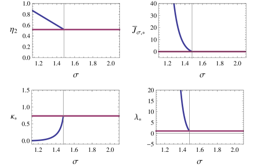
The first possibility is $\bar{J}_{\sigma}^{*}=0$ and we are in the SR case, the second is $\eta_{2}=2-\sigma$ which is a characteristic of the LR fixed point, a least at this approximation level.

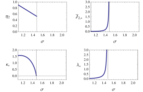
Figure 6: Anomalous dimension $\eta_{2}$ and fixed point values $J_{\sigma,*}$,$\kappa_{*}$,$\lambda_{*}$ in the truncation considered in the text. For $\sigma>\sigma_{*}\equiv 2-\eta_{SR}$ only the fixed point (red line) is present characterized by $\eta_{2}=\eta_{SR}$ and $J_{\sigma,*}=0$. At $\sigma=\sigma_{*}$ the LR fixed point (blue lines) branches from the SR fixed point and then controls the critical behaviour for every $\sigma<\sigma_{*}$. Thus even in the case of both SR and LR terms in the propagator the anomalous dimension as a function of $\sigma$ is thus LR ($\eta_{2}=2-\sigma$) for $\sigma<\sigma_{*}$ and SR for $\sigma>\sigma_{*}$.

This shows that we have no necessity to change the field dimension to study the case of a dominant LR term, since the $p^{2}$ term is still present in the LR fixed point.
In order to check these properties we turn to the approximation where we expand the potential around its minimum:

$$\bar{U}_{k}(\bar{\rho})=\frac{1}{2}\lambda_{k}(\bar{\rho}-\kappa_{k})^{2}\,.$$ (35)

Projecting the flow equation for the potential we can get the beta functions of these two couplings which, together with the flow equation for $\bar{J}_{\sigma}$, form a closed set:

$$\partial_{t}\bar{J}_{\sigma}=(\sigma-2)\bar{J}_{\sigma}+\eta_{2}\bar{J}_{\sigma}\,,$$ (36a)

$$\eta_{2}=\frac{(2+\sigma\bar{J}_{\sigma})^{2}\kappa_{k}\lambda_{k}^{2}}{(1+\bar{J}_{\sigma})^{2}(1+\bar{J}_{\sigma}+2\kappa_{k}\lambda_{k})^{2}}\,,$$ (36b)

$$\partial_{t}\kappa_{k}=\;-(d-2+\eta_{2})\kappa_{k}+3\frac{1-\frac{\eta_{2}}{d+2}+\frac{\sigma}{2}\bar{J}_{\sigma}}{(1+\bar{J}_{\sigma}+2\kappa_{k}\lambda_{k})^{2}}+(N-1)\frac{1-\frac{\eta_{2}}{d+2}+\frac{\sigma}{2}\bar{J}_{\sigma}}{(1+\bar{J}_{\sigma})^{2}}\,,$$ (36c)

$$\partial_{t}\lambda_{k}=(d-4+2\eta_{2})\lambda_{k}+18\lambda_{k}\frac{1-\frac{\eta_{2}}{d+2}+\frac{\sigma}{2}\bar{J}_{\sigma}}{(1+\bar{J}_{\sigma}+2\kappa_{k}\lambda_{k})^{3}}+2\lambda_{k}(N-1)\frac{1-\frac{\eta_{2}}{d+2}+\frac{\sigma}{2}\bar{J}_{\sigma}}{(1+\bar{J}_{\sigma})^{3}}\,.$$ (36d)

As discussed SR-dimensions are well suited to study the case $\sigma<\sigma_{*}$, since $Z_{2}$ is well defined in this case and is not brought to zero by the presence of a dominant LR term. The results for the couplings and the anomalous dimension at the fixed point is shown in Fig.6. We see that the anomalous dimension $\eta_{2}$ follows naturally the Sak’s behaviour with no possible LR fixed point solution for $\sigma>\sigma_{*}$, however at $\sigma=\sigma_{*}$ the LR fixed point (blue lines) appears and the value of the coupling in that point is shown. It is possible to see that the $\bar{J}_{\sigma,*}$ grows very fast when we approach $\sigma=d/2$ (which is $1$ in this case since we are plotting $2$ dimensional results). This coupling is actually diverging at $\sigma=1$ since at the point the LR fixed point merges with the Gaussian LR fixed point, which can be suitably described only in LR-dimensions, since it has no SR term in its propagator. This has been verified for different values of $\sigma>\sigma_{*}$, at different (also non-integer) dimensions and for various $O(N)$ models. It is also possible to show that the truncation of the potentials despite changing the value of any quantity at the fixed point does not modify the qualitative behaviour of the system nor the existence of the threshold $\sigma_{*}$.

Figure 7: Anomalous dimension $\eta_{2}$ and fixed point values $\bar{J}_{\sigma,*},\kappa_{*},\lambda_{*}$ in the truncation (27) with LR–dimensions. With this dimensional choice we are able to describe only the $\sigma<\sigma_{*}$ region, since in the other region the coupling $\bar{J}_{2,k}$ is divergent, as can be understood from the $\bar{J}_{2,k}$ plot. Also in this case, the anomalous dimension as a function of $\sigma$ is LR ($\eta_{2}=2-\sigma$) for $\sigma<\sigma_{*}$.

LR–Dimensions

Here for the sake of completeness we also report the results obtained using LR dimensionless variables. In this case we renormalize the field using the wave function $Z_{\sigma}$ and we define the SR coupling $\bar{J}_{2}=\bar{Z}_{2}/Z_{\sigma}$

$$\partial_{t}Z_{\sigma}=0\,,$$ (37a)

$$\partial_{t}\bar{J}_{2}=(2-\sigma)\bar{J}_{2}-\frac{\bar{\rho}_{0}\,\bar{U}^{\prime\prime}_{k}(\bar{\rho}_{0})^{2}(\sigma+2\bar{J}_{2})^{2}}{(1+\bar{J}_{2})^{2}(1+\bar{J}_{2}+2\kappa_{k}\bar{U}^{\prime\prime}_{k}(\bar{\rho}_{0}))^{2}}\,,$$ (37b)

$$\begin{split}\partial_{t}U_{k}(\rho)=&-d\bar{U}_{k}(\bar{\rho})+(d-\sigma)\bar{\rho}\,\bar{U}^{\prime}_{k}(\bar{\rho})+\frac{\bar{J}_{2}-\frac{(2-\sigma)\bar{J}_{2}+\partial_{t}\bar{J}_{2}}{d+2}+\frac{\sigma}{2}}{1+\bar{J}_{2}+\bar{U}^{\prime}_{k}(\bar{\rho})+2\bar{\rho}\,\bar{U}^{\prime\prime}_{k}(\bar{\rho})}\\ &+(N-1)\frac{\bar{J}_{2}-\frac{(2-\sigma)\bar{J}_{2}+\partial_{t}\bar{J}_{2}}{d+2}+\frac{\sigma}{2}}{1+\bar{J}_{2}+\bar{U}^{\prime}_{k}(\bar{\rho})}\,.\end{split}$$ (37c)

These equations in the $\bar{J}_{2}\rightarrow 0$ limit reproduce the results obtained for previous the approximations. Thus this approximation reproduces, as expected, all the previous results in the range $\sigma<\sigma_{*}$, but also gives information on their validity, comparing latter equation with (18) we see that they are equal up to a term of order $\bar{J}_{2}$. In fact if we use LR-dimensions we find coherently that $\bar{J}_{2}^{*}\neq 0$ is very small for all $\sigma<\sigma_{*}$ but in the region $\sigma\simeq\sigma_{*}$, when as we expected the effective dimension relations are spoiled (this is shown in Fig.7).

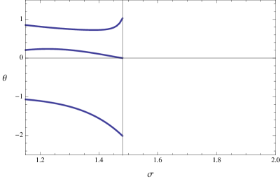
Figure 8: Eigenvalues ($\theta$) of the RG stability matrix as a function of $\sigma$ for the LR (blue lines) fixed points in the case of LR-dimensions. In this case we are not able to describe only the LR fixed point present when $\sigma<\sigma_{*}$ and,since RG eigenvalues are universal quantities, they agree with SR-dimensions ones.

We can then repeat the previous analysis. We have in this case one, very important, difference: we are renormalizing the field with the $Z_{\sigma}$ wave function. This is consistent in the range $\sigma<\sigma_{*}$ where the LR interaction, while in the case of a dominant $p^{2}$ interaction ($\sigma>\sigma_{*}$) we expect the $Z_{2}$ wave function to be diverging, this divergence is not absorbed in the field as an anomalous dimension and cannot be balanced by $Z_{\sigma}$ which we know to be constant at this approximation level. Thus this divergence will still be present in our flow and this choice for the dimensionless coupling is not suited in the case $\sigma>\sigma_{*}$ (Fig. 7).

We then investigate the case $\sigma<\sigma_{*}$ where our variable are well defined, as usual we refer to the very simple truncation shown in Eq. (35) and we use the renormalization time $t=\log(k/k_{0})$. The flow equations are:

$$\begin{split}\partial_{t}\bar{J}_{2}=(2-\sigma)\bar{J}_{2}+\frac{\kappa_{k}\lambda_{k}^{2}(\sigma+2\bar{J}_{2})^{2}}{(1+\bar{J}_{2})^{2}(1+\bar{J}_{2}+2\kappa_{k}\lambda_{k})^{2}}\,,\end{split}$$ (38a)

$$\begin{split}\partial_{t}\kappa_{k}=&\;-(d-\sigma)\kappa_{k}+3\frac{\bar{J}_{2}-\frac{(2-\sigma)\bar{J}_{2}+\partial_{t}\bar{J}_{2}}{d+2}+\frac{\sigma}{2}}{(1+\bar{J}_{2}+2\kappa_{k}\lambda_{k})^{2}}\\ &+(N-1)\frac{\bar{J}_{2}-\frac{(2-\sigma)\bar{J}_{2}+\partial_{t}\bar{J}_{2}}{d+2}+\frac{\sigma}{2}}{(1+\bar{J}_{2})^{2}}\,,\end{split}$$ (38b)

$$\begin{split}\partial_{t}\lambda_{k}=&\;(d-2\sigma)\lambda_{k}+18\lambda_{k}\frac{\bar{J}_{2}-\frac{(2-\sigma)\bar{J}_{2}+\partial_{t}\bar{J}_{2}}{d+2}+\frac{\sigma}{2}}{(1+\bar{J}_{2}+2\kappa_{k}\lambda_{k})^{3}}\\ &+2\lambda_{k}(N-1)\frac{\bar{J}_{2}-\frac{(2-\sigma)\bar{J}_{2}+\partial_{t}\bar{J}_{2}}{d+2}+\frac{\sigma}{2}}{(1+\bar{J}_{2})^{3}}\,.\end{split}$$ (38c)

The fixed points solutions of the couplings is reported in Fig. 7, where we see that only the LR fixed points solution are present and then only the region $\sigma<\sigma_{*}$ is investigated. In fact, as well as previous couplings showed a diverging $\bar{J}_{\sigma,*}$ for $\sigma\to 1$, these couplings show a divergence in the limit $\sigma\to\sigma_{*}$ where the LR term in the propagator is vanishing. However the results for the critical exponents in the region where both the couplings sets are defined are in perfect agreement between themselves, as it should be and as it is shown in Fig.8.

References

• (1) Long-Range Interacting Systems: Lecture Notes of Les Houches Summer School, T. Dauxois, S. Ruffo, and L. F. Cugliandolo eds. (Oxford, Oxford University Press, 2010).
• (2) F. J. Dyson, Comm. Math. Phys. 12, 91 (1969).
• (3) D. J. Thouless, Phys. Rev. 187, 732 (1969).
• (4) P. W. Anderson, G. Yuval, and D. R. Hamann, Phys. Rev. B 1, 4464 (1970).
• (5) A. Campa, T. Dauxois, and S. Ruffo, Phys. Rep. 480, 57 (2009).
• (6) M. E. Fisher, S. K. Ma, and B. G. Nickel, Phys. Rev. Lett. 29, 14 (1972).
• (7) J. Sak, Phys. Rev. B 8, 281 (1973).
• (8) J. L. Cardy, J. Phys. A 14, 1407 (1981).
• (9) J. FrΓΆlich and T. Spencer, Comm. Math. Phys. 84, 87 (1982).
• (10) E. Luijten and H. Messingfeld, Phys. Rev. Lett. 86, 5305 (2001).
• (11) E. Luijten, Interaction Range, universality and the Upper Critical Dimension, Ph. D. Thesis (1997).
• (12) E. Luijten and H. W. J. BlΓΆte, Int. J. Mod. Phys. C 6, 359 (1995).
• (13) E. Luijten and H. W. J. BlΓΆte, Phys. Rev. Lett. 89, 025703 (2002).
• (14) M. Picco, arXiv:1207.1018
• (15) T. Blanchard, M. Picco, and M. A. Rajapbour, Europhys. Lett. 101, 56003 (2013).
• (16) P. Grassberger, arXiv:1305.5940
• (17) M. C. Angelini, G. Parisi, and F. Ricci-Tersenghi, Phys. Rev. E 89, 062120 (2014).
• (18) J. Berges, N. Tetradis, and C. Wetterich, Phys. Rep. 363, 223 (2002).
• (19) B. Delamotte, in Order, disorder and criticality: advanced problems of phase transition theory, Yu. Holovatch ed. (Singapore, World Scientific, 2007) [arXiv:cond-mat/0702365].
• (20) A. Codello and G. D’Odorico, Phys. Rev. Lett. 110, 141601 (2013).
• (21) A. Codello, N. Defenu, and G. D’Odorico, arXiv:1410.3308
• (22) C. Wetterich, Phys. Lett. B 301, 90 (1993).
• (23) A. Codello, J. Phys. A 45, 465006 (2012).
• (24) T. R. Morris, Phys. Lett. B 334, 355 (1994).
• (25) G. S. Joyce, in Phase Transitions and Critical Phenomena vol. 2, C. Domb and M. S. Green eds., pp. 375-442 (London, Academic Press, 1972).
• (26) N. Tetradis and C. Wetterich, Nucl. Phys. B 422, 541 (1994).
• (27) H. E. Stanley, Phys. Rev. 176, 718 (1968).
• (28) R. A. BaΓ±os, L. A. Fernandez, V. Martin-Mayor, and A. P. Young, Phys. Rev. B 86, 134416 (2012).
• (29) S. L. Katz, M. Droz, and J. D. Gunton, Phys. Rev. B 15, 1597 (1977).
• (30) Yu. Holovatch, Int. J. Mod. Phys. A 8, 5329 (1993).
• (31) S. El-Showk, M. Paulos, D. Poland, S. Rychkov, D. Simmons-Dun, and A. Vichi, Phys. Rev. Lett. 112, 141601 (2014).
• (32) M. Baczyk, M. Tissier, G. Tarjus, and Y. Sakamoto Phys. Rev. B 88, 014204 (2013).
• (33) I. Balog, G. Tarjus, and M. Tissier J. Stat. Mech. P10017 (2014).
• (34) E. Brezin, G. Parisi, and F. Ricci-Tersenghi arXiv:1407.3358.