Strong Steiner Tree Approximations in Practice

Abstract

In this experimental study we consider Steiner tree approximation algorithms that guarantee a constant approximation ratio smaller than $2$. The considered greedy algorithms and approaches based on linear programming involve the incorporation of $k$-restricted full components for some $k\geq 3$. For most of the algorithms, their strongest theoretical approximation bounds are only achieved for $k\to\infty$. However, the running time is also exponentially dependent on $k$, so only small $k$ are tractable in practice.

We investigate different implementation aspects and parameter choices that finally allow us to construct algorithms (somewhat) feasible for practical use. We compare the algorithms against each other, to an exact LP-based algorithm, and to fast and simple $2$-approximations.

Funded by the German Research Foundation (DFG), project number CH 897/1-1.
Preliminary versions of this work appeared as [Chimani and Woste 2011] and [Beyer and Chimani 2014].

1 Introduction

The Steiner tree problem, essentially asking for the cheapest connection of points in a metric space, is a fundamental problem in computer science and operations research. In the general setting, we are given a connected graph $G=(V,E)$ with edge costs ${d}\colon{E}\to{\mathbb{R}_{\geq 0}}$ and a subset $R\subseteq V$ of nodes. Those required nodes $R$ are called terminals, and $V\setminus R$ are called nonterminals. A terminal-spanning subtree in $G$ is called a Steiner tree. The minimum Steiner tree problem in graphs (STP) is to find a Steiner tree $T=(V_{T},E_{T})$ in $G$ with $R\subseteq V_{T}\subseteq V$ and minimizing the cost $d(T):=d(E_{T}):=\sum_{e\in E_{T}}{d(e)}$.

As one of the hard problems identified by Karp [1972], the STP is even NP-hard for special cases like bipartite graphs with uniform costs [Hwang et al. 1992]. Papadimitriou and Yannakakis [1988] proved that the STP is in MAX SNP, Bern and Plassmann [1989] showed that this is even the case if edge costs are limited to $1$ and $2$. No problem in MAX SNP has a polynomial-time approximation scheme (PTAS) if $\textsf{P}\neq\textsf{NP}$, that is, it cannot be approximated arbitrarily close to ratio $1$ in polynomial time under widespread assumptions. The best known lower bound for an approximation ratio is $96/95\approx 1.0105$ [Chlebík and Chlebíková 2008].

The STP has various applications in the fields of VLSI design, routing, network design, computational biology, and computer-aided design. It serves as a basis for generalized problems like prize-collecting and stochastic Steiner trees, Steiner forests, Survivable Network Design problems, discount-augmented problems like Buy-at-Bulk or Rent-or-Buy, and appears as a subproblem in problems like the Steiner packing problem.

The versatile applicability of the STP gave rise to a lot of research from virtually all algorithmic points of view: heuristics, metaheuristics, and approximation algorithms [Rayward-Smith 1983, Kahng and Robins 1992, Gubichev and Neumann 2012, Poggi de Aragão et al. 2001, Leitner et al. 2014, Takahashi and Matsuyama 1980, Kou et al. 1981, Mehlhorn 1988, Zelikovsky 1992; 1993a; 1993b, Berman and Ramaiyer 1994, Goemans and Williamson 1995, Zelikovsky 1995, Karpinski and Zelikovsky 1995, Prömel and Steger 1997, Hougardy and Prömel 1999, Robins and Zelikovsky 2005, Byrka et al. 2013, Goemans et al. 2012] on the one side and exact algorithms based on branch-and-bound, dynamic programming, fixed-parameter tractability, and integer linear programs [Shore et al. 1982, Dreyfus and Wagner 1972, Hougardy et al. 2014, Vygen 2011, Chimani et al. 2012, Fafianie et al. 2013, Aneja 1980, Wong 1984, Polzin and Vahdati Daneshmand 2001] on the other side. Both areas are complemented by research about reduction techniques on the problem [Duin and Volgenant 1989, Polzin and Vahdati Daneshmand 2002]. However, by far not all of that research is backed by experimental studies. This paper attempts to close this gap in the field of strong approximation algorithms where there has only been the preliminary conference papers leading to this article [2011, 2014], and the work of Ciebiera et al. [2014] during the 11th DIMACS Implementation Challenge [2014]. By strong approximations we denote approximations with ratio smaller than $2$. Although those algorithms have been a breakthrough in theory, their actual practicability has remained unclear. We contribute by implementing, extending, evaluating, and comparing the different strong algorithms and a variety of algorithmic variants thereof. We also compare them to simple $2$-approximations and exact algorithms.

In the following section we first give an overview on the basic ideas behind strong algorithms and their evolution. We then describe the two known classes of algorithms, greedy combinatorial algorithms and LP-based algorithms, in more detail. We only give as many details as necessary to understand our subsequent design choices and algorithm variants. Section 3 is about different practical variants for the algorithms. In Section 4 we evaluate the algorithms and their variants, and compare their running times and solution qualities to basic $2$-approximations and an exact algorithm.

2 The Algorithms

For any graph $H$, we denote its nodes by $V_{H}$, its edges by $E_{H}$, and its terminals by $R_{H}$. When referring to the input graph $G$, we omit the subscript. By $\textrm{MST}(H)$ we denote a minimum spanning tree in $H$. Let $\bar{G}$ be the metric closure of $G$, that is, the complete graph on $V$ such that the cost of each edge $\{u,v\}$ is the minimum cost of any $u$-$v$-path in $G$. Let $\bar{G}_{U}$ denote the $U$-induced subgraph of $\bar{G}$ for $U\subseteq V$. For any graph $G$ and any subgraph $H\subseteq G$, we denote by $G/H$ the result of contracting $H$ into a single node in $G$.

We first give an overview on purely combinatorial approximation algorithms for the STP describing the basic ideas coarsely. In Section 2.1 we provide a more detailed description of some of the formerly strongest approximation algorithms. Section 2.2 is about recent approximation algorithms that are based on linear programming techniques.

The simplest algorithms are basic $2$-approximations. The algorithm by Takahashi and Matsuyama [1980] can be compared to the Jarník-Prim algorithm to find minimum spanning trees. In each iteration, a shortest path to an unvisited terminal (instead of a single edge to an unvisited node) is added. That is, the algorithm builds the Steiner tree starting with a single terminal node and iteratively adds the shortest path to the nearest terminal to the tree. The algorithm by Kou et al. [1981] computes $\bar{G}_{R}$ and $\textrm{MST}(\bar{G}_{R})$. After replacing the edges of $\textrm{MST}(\bar{G}_{R})$ by the corresponding shortest paths in $G$, and cleaning up the obtained graph (i.e., breaking possible cycles and pruning Steiner leaves), we obtain a Steiner tree that is a $2$-approximation. Mehlhorn [1988] suggests a more time-efficient variant that exploits the use of Voronoi regions.

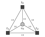
(a) The instance.

(b) Possible result of $2$-approximations.

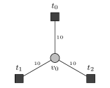
(c) Improved approximation (and optimum solution).

Figure 1: A simple example that shows how converting a well-chosen nonterminal (here $v_{0}$) to a terminal can improve a $2$-approximation. Square nodes are terminals, circular nodes are nonterminals.

Assume we want to improve a Steiner tree $T$ that is obtained by a $2$-approximation. One idea is to find nonterminals that are not already included in $T$ but whose inclusion would improve $T$. Hence, by temporarily converting these nonterminals to terminals and applying a $2$-approximation on the new instance, the result can be better. Fig. 1 shows such a case. The crucial ingredient in this idea is the choice of the nonterminals. Zelikovsky [1992, 1993a, 1993b] gives an approach that guarantees an approximation ratio of $11/6$. For every choice of three terminals, his algorithms find a nonterminal to be chosen as the center of a star where the three terminals are the leaves. Among all these stars, the “best” ones—according to some greedy criterion function—are chosen for the Steiner tree to be constructed.

From another point of view, this approach exploits the decomposition of a Steiner tree into full components, a concept already mentioned by Gilbert and Pollak [1968]. A Steiner tree is full if its set of leaves coincides with its set of terminals. Any Steiner tree can be uniquely decomposed into full components by splitting up inner terminals. We say a $k$-restricted component is a full component with at most $k$ leaves and a $k$-component is a full component with exactly $k$ leaves. A $k$-restricted Steiner tree is a Steiner tree where each component is $k$-restricted. In these terms, the algorithm by Kou et al. [1981] is a Steiner tree construction using $2$-components, and the mentioned algorithms by Zelikovsky use $3$-restricted components.

All strong algorithms for the STP known so far exploit the decomposition of a Steiner tree into full components by first constructing a set of $k$-restricted components and then putting the full components together to obtain a $k$-restricted Steiner tree. Interestingly, the cost ratio between a minimum $k$-restricted Steiner tree and a minimum Steiner tree is (tightly) bounded by $\varrho_{k}:=1+\frac{2^{r}}{(r-1)\,2^{r}+k}$ with $r=\lfloor\log_{2}{k}\rfloor$ Borchers and Du [1995]. Note that $\varrho_{2}=2$ is also the approximation ratio for approximations based on $2$-restricted Steiner trees since the minimum $2$-restricted Steiner tree of a graph corresponds to the back-transformation of $\textrm{MST}(\bar{G}_{R})$. However, $\varrho_{k}$ for $k\geq 3$ cannot simply serve as an approximation ratio: it is not known whether a polynomial-time algorithm for $k=3$ exists. However, there is a PTAS for this case [Prömel and Steger 1997], so it is possible to approximate arbitrarily close to ratio $\varrho_{3}=5/3$. Obtaining a minimum $k$-restricted Steiner tree for $k\geq 4$ is strongly NP-hard, as follows from a trivial reduction from Exact Cover by $r$-Sets with $r=k-1$.

With respect to $\varrho_{k}$, Zelikovsky’s approach yields an approximation ratio of $\frac{\varrho_{2}+\varrho_{3}}{2}=\frac{11}{6}$. Berman and Ramaiyer [1994] were the first to generalize this approach to arbitrary $k$ by using rather complicated preselection and construction phases. They obtain a ratio of $\varrho_{2}-\sum_{i=3}^{k}\frac{\varrho_{i-1}-\varrho_{i}}{i-1}\geq 1.7333$ but, in particular, $11/6\approx 1.8333$ for $k=3$ and $16/9\approx 1.7778$ for $k=4$. Zelikovsky [1995] generalizes his former approach using another greedy selection criterion (the relative greedy heuristic) and obtains an approximation ratio of $(1+\ln{\frac{\varrho_{2}}{\varrho_{k}}})\varrho_{k}\approx(1.693-\ln\varrho_{k})\varrho_{k}$ which becomes approximately $1.693$ for $k\to\infty$ since $\varrho_{k}$ tends to $1$. However, the proven approximation ratios for $k=3,4$ are only about $1.97$ and $1.93$, respectively.

Karpinski and Zelikovsky [1995] introduce the notion of the loss of a full component to allow some more sophisticated preprocessing. They utilize it to prove small improvements for the Berman-Ramaiyer algorithm with $k=4$ (from $1.778$ to $1.757$) and for the relative greedy heuristic with $k\to\infty$ (from $1.693$ to $1.644$). Hougardy and Prömel [1999] use the idea of Karpinsky and Zelikovsky in an iterated manner. They incorporate the loss of a full component with some well-chosen weight into the relative greedy heuristic and solve it to obtain a Steiner tree. In each iteration, the weight is decreased and the modified relative greedy heuristic is run again. The optimal sequence of weights can be found using numerical optimization. For 11 iterations and $k\to\infty$, they obtain an approximation ratio of $1.598$.

Prömel and Steger [1997] use algebraic techniques to attack the problem of obtaining a minimum $3$-restricted Steiner tree. They obtain a randomized fully polynomial-time $(\varrho_{3}+\varepsilon)$-approximation scheme, however, with a sequential time complexity of $\mathcal{O}\!\left(\frac{\log(1/\varepsilon)}{\varepsilon}n^{11+\omega}\log{n}\right)$ where $\omega$ is the exponent of matrix multiplication.

The so far best purely combinatorial approximation algorithm is the loss-contracting algorithm by Robins and Zelikovsky [2005]. The obtained approximation ratio is $(1+\frac{1}{2}\ln(\frac{4}{\varrho_{k}}-1))\varrho_{k}$ which tends to $1.549$ for $k\to\infty$ and is $1.947$ and $1.883$ for $k=3,4$, respectively. We will describe it in more detail in the following section, before discussing the even stronger LP-based algorithms in Section 2.2.

2.1 Greedy Contraction Framework

A lot of the strong algorithms are based on the contraction of full components. The idea behind all these algorithms is basically the same. It was first summarized by Zelikovsky [1995] and called the greedy contraction framework (GCF).

We are (implicitly or explicitly) given a list $\mathcal{C}_{k}$ of $k$-restricted components and a win function $\textit{win}_{f}$ that characterizes the benefit of choosing a full component in the final Steiner tree. Its value for a specific full component $C$ is called win, and we call $C$ promising if choosing $C$ guarantees an improvement. The GCF begins by computing the metric closure $M:=\bar{G}_{R}$ over the terminals $R$ in $G$. Recall that deducing a Steiner tree from $\textrm{MST}(\bar{G}_{R})$ yields a $2$-approximation. Iteratively, the GCF finds a full component $C\in\mathcal{C}_{k}$ that maximizes $\textit{win}_{f}(M,C)$, and contracts $C$ in $M$ if this win is promising. This process is repeated as long as there are full components with promising wins.

Each time a full component is contracted, it is incorporated into the final Steiner tree. This can be done by converting the nonterminals of the chosen full components into terminal nodes and computing a $2$-approximation using the new terminal node set. Alternatively, we can start with an empty graph $T$, inserting each chosen full component into $T$, and finally returning $\textrm{MST}(T)$ to clean up cycles that may have arisen (see [Zelikovsky 1995, Robins and Zelikovsky 2005]).

The loss-contracting algorithm (LCA) by Robins and Zelikovsky [2005] is a variant of GCF with a small difference: not the whole full component is contracted but only its loss.

Definition 1 (core edges, loss).

We denote as core edges of $C$ a minimal subset of $E_{C}$ whose removal disconnects all terminals in $C$. The loss $\textit{Loss}(C)$ of a full component $C$ is the minimum-cost subforest of $C$ such that all inner nodes are connected to leaves.

A full component with $k$ leaves has exactly $k-1$ core edges. Note that the definition of core edges does not involve edge costs. The complement of any spanning tree in $C/R_{C}$ forms a set of core edges. $\textit{Loss}(C)$, however, is a minimum spanning tree in $C/R_{C}$. Overall, the set of non-loss edges (the complement of $\textit{Loss}(C)$) is one possible core edge set (but not the only one). This distinction will become relevant for the randomized algorithm described in Section 2.2. When computing $\textit{Loss}(C)$, it is sufficient to insert zero-cost edges between all terminals $R_{C}$ into $C$ instead of considering the $C/R_{C}$ contraction, see [Robins and Zelikovsky 2005, Lemma 2].

The idea behind the LCA in contrast to the GCF is to leave out high-cost edges as long as they are not necessary to connect the solution. From another point of view, this allows the algorithm to reject edges in a full component after a full component has already been accepted for inclusion.

In order to be able to perform a loss-contraction, the full component has to be included into $M$ first. Hence $M/\textit{Loss}(C)$ is short-hand for $(M\cup C)/\textit{Loss}(C)$. Since only the MSTs of the contracted graphs are necessary, we can perform a contraction by adding zero-cost edges between contracted terminals, and a loss-contraction by adding the non-loss edges. Figure 2 illustrates the difference of a contraction and a loss-contraction.

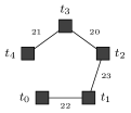
(a) $\textrm{MST}(M)$

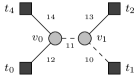
(b) Full component $C$ to be selected. Dashed lines denote loss edges.

(c) $\textrm{MST}(M/C)$

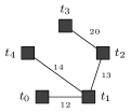
(d) $\textrm{MST}(M/\textit{Loss}(C))$

Figure 2: An example showing the difference between a contraction (using zero-cost edges) and a loss-contraction of a full component.

Among the purely combinatorial algorithms, the GCF and its variant LCA are the ones we will focus on. We refrain from explicitly implementing the mentioned GCF variants involving iterative and preprocessing techniques as they are either impractical [Hougardy and Prömel 1999] or dominated by other methods [Berman and Ramaiyer 1994, Karpinski and Zelikovsky 1995]. Also the algebraic approach [Prömel and Steger 1997] for the $3$-restricted case is clearly impractical.

Win functions.

One crucial ingredient of many win functions is the save. When inserting a full component $C$ into $\textrm{MST}(M)$, we obtain cycles. Those cycles can be broken by deleting the maximum-cost edges in these cycles. We call those edges save edges, and their total cost is the save. Formally, let $\textit{save}_{M}(u,v)$ be the maximum-cost edge on the unique path between $u,v\in\textrm{MST}(M)$, and let $\textit{save}(M,C):=d(\textrm{MST}(M))-d(\textrm{MST}(M/C))$ denote the cost difference between the minimum spanning trees in $M$ and $M/C$.

Several win functions have been proposed. Zelikovsky originally suggested the absolute win function $\textit{win}_{\text{abs}}(M,C):=\textit{save}(M,C)-d(C)$ that describes the actual cost reduction of $M$ when we include $C$. Using $\textit{win}_{\text{abs}}$ yields an $11/6$-approximation for $k=3$ [Zelikovsky 1992; 1993a; 1993b]. The relative win function $\textit{win}_{\text{rel}}(M,C):=\frac{\textit{save}(M,C)}{d(C)}$ achieves approximation ratio $1.69$ for $k\to\infty$ [Zelikovsky 1995].

For the LCA, Robins and Zelikovsky [2005] proposed $\textit{win}_{\text{loss}}(M,C):=\frac{\textit{win}_{\text{abs}}(M,C)}{d(\textit{Loss}(C))}$. It relates the cost reduction from the choice of a full component to the cost of connecting their nonterminals to terminals, which is the actual cost when contracting the loss of a full component. In their survey, Gröpl et al. [2001] used $\textit{win}_{\text{loss}^{\prime}}(M,C):=\frac{\textit{save}(M,\textit{Loss}(C))}{d(\textit{Loss}(C))}$ that coincides with $\textit{win}_{\text{loss}}(M,C)+1$ since $d(\textrm{MST}(M/\textit{Loss}(C)))=d(\textrm{MST}(M/C))+d(C)-d(\textit{Loss}(C))$. We see that $\textit{win}_{\text{loss}}$ is conceptually a direct transfer of $\textit{win}_{\text{rel}}$ to the case of loss contractions. It guarantees an $\approx 1.549$ approximation ratio for $k\to\infty$.

The GCF loop terminates when no promising full component has been found, that is, when the choice of a full component $C$ with maximum win does not improve $M$. This is the case if $\textit{win}_{\text{abs}}(M,C)\leq 0$ (and hence $\textit{win}_{\text{loss}}(M,C)\leq 0$) or $\textit{win}_{\text{rel}}(M,C)\leq 1$ for all $C\in\mathcal{C}_{k}$.

2.2 Algorithms Based on Linear Programming

In contrast to the purely combinatorial algorithms above, there are also approximation algorithms based on linear programming.

The primal-dual algorithm by Goemans and Williamson [1995] for constrained forest problems can be applied to the STP but only yields a $2$-approximation. It is based on the undirected cut relaxation (UCR) with a tight integrality gap of $2$. We obtain the bidirected cut relaxation (BCR) by transforming $G$ into a bidirected graph. Let $A:=\{{(u,v),(v,u)}\,\mid\,{e=\{u,v\}\in E}\}$ denote the arc set of $G$, and let $\delta^{-}({U}):=\{{(u,v)\in A}\,\mid\,{u\in U\setminus{V},v\in U}\}$ be the set of arcs entering $U\subseteq V$. The cost of each arc coincides with the cost of the corresponding edge. BCR is defined as:

min $$\sum_{e\in A}{d(e)\,x_{e}}$$ (BCR)

s. t. $$\sum_{e\in\delta^{-}({U})}{x_{e}}\,\geq\,1, U\subsetneq V r\in U\cap R\neq R$$ for all with , (1a)

$$0\leq x_{e}\leq 1\text{,} e\in A$$ for all (1b)

where $r\in R$ is an arbitrary (fixed) root terminal. We obtain the ILP of BCR by requiring integrality for $x$ (and analogously for the relaxations below). Clearly, every feasible solution of the ILP spans all terminals: the directed cut constraint (1a) guarantees that there is at least one directed path from any terminal to $r$. Since every optimal solution represents a tree where all arcs are directed towards $r$, dropping the directions of that arborescence yields a minimum-cost Steiner tree. Although BCR is strictly stronger than UCR, no BCR-based approximation with ratio smaller than $2$ is known.

Byrka et al. [2013] incorporate the idea of using $k$-restricted components to find the directed-component cut relaxation (DCR). They prove an upper bound of the integrality gap of $1+\frac{\ln{3}}{2}\approx 1.55$ for $k\to\infty$ and obtain an approximation algorithm with approximation ratio at most $\varrho_{k}\ln{4}$ that tends to $\approx 1.39$ for $k\to\infty$. Let $\mathcal{D}_{k}$ denote the set of directed full components obtained from $\mathcal{C}_{k}$: For each $C\in\mathcal{C}_{k}$ with $R_{C}=\{v_{1},\ldots,v_{|R_{C}|}\}$, we make $|R_{C}|$ copies of $C$ and direct all edges in the $i$-th copy of $C$ towards $v_{i}$ for $i=1,\ldots,|R_{C}|$. For each $D\in\mathcal{D}_{k}$ let $t_{D}$ be the node all edges are directed to. Let $\tilde{\delta}^{-}({U}):=\{{D\in\mathcal{D}_{k}}\,\mid\,{U\setminus R_{D}\neq\emptyset,t_{D}\in U}\}$ be the set of directed full components entering $U\subseteq R$. DCR is defined as:

min $$\sum_{D\in\mathcal{D}_{k}}{d(D)\,x_{D}}$$ (DCR)

s. t. $$\sum_{D\in\tilde{\delta}^{-}({U})}{x_{D}}\,\geq\,1, U\subsetneq R r\in U$$ for all with , (2a)

$$0\leq x_{D}\leq 1\text{,} D\in\mathcal{D}_{k}$$ for all (2b)

where $r\in R$ is again an arbitrary root. The approximation algorithm iteratively solves DCR, samples a full component $D$ according to a probability distribution based on the solution vector, contracts $D$, and iterates this process by resolving the new DCR instance. The algorithm stops when all terminals are contracted. The union of the chosen full components represents the resulting $k$-restricted Steiner tree. Although the sampling of the full components is originally randomized, a derandomization of the algorithm is possible.

Warme [1998] showed that constructing a minimum $k$-restricted Steiner tree is equivalent of finding a minimum spanning tree in the hypergraph $(R,\{{R_{C}}\,\mid\,{C\in\mathcal{C}_{k}}\})$, i.e., the terminals represent the nodes of the hypergraph and the full components represent the hyperedges. He introduced the following relaxation:

min $$\sum_{C\in\mathcal{C}_{k}}{d(C)\,x_{C}}$$ (SER)

s. t. $$\sum_{C\in\mathcal{C}_{k}}{(|R_{C}|-1)\,x_{C}}\,=\,|R|-1,$$ (3a)

$$\sum_{\begin{subarray}{c}C\in\mathcal{C}_{k}\\ R^{\prime}\cap R_{C}\neq\emptyset\end{subarray}}{(|R^{\prime}\cap R_{C}|-1)\,x_{C}}\,\leq\,|R^{\prime}|-1, R^{\prime}\subseteq R,|R^{\prime}|\geq 2$$ for all , (3b)

$$0\leq x_{C}\leq 1\text{,} C\in\mathcal{C}_{k}$$ for all . (3c)

Constraint (3a) represents the basic relation between the number of nodes and edges in hypertrees (like $|E|=|V|-1$ in trees). Since arbitrary subsets of nodes are not necessarily connected but cycle-free, this directly implies the subtour elimination constraints (3b). We call that relaxation the subtour elimination relaxation (SER).

Polzin and Vahdati Daneshmand [2003] proved that DCR and SER are equivalent. Könemann et al. [2011] and Chakrabarty et al. [2010a] also provided partition-based relaxations that are equivalent to DCR and SER. All these equivalent LP relaxations are summarized as hypergraphic relaxations.

Chakrabarty et al. [2010b] developed an $1.55$-approximation algorithm for $k\to\infty$ based on SER to prove the integrality gap of DCR in a simpler way than Byrka et al. [2013]. Their algorithm has the advantage that it only solves the LP relaxation once instead of solving new LP relaxations after each single contraction. This improves the running times. The disadvantage is that the approximation ratio is not better than the purely combinatorial algorithm by Robins and Zelikovsky [2005].

Goemans et al. [2012] used techniques from the theory of matroids and submodular functions to improve the upper bound on the integrality gap of the hypergraphic relaxations such that it matches the ratio $1.39$ of the approximation algorithm by Byrka et al. [2013]. They found a new approximation algorithm that solves the hypergraphic relaxation once and builds an auxiliary directed graph from the solution. Full components in that auxiliary graph are carefully selected and contracted, until the auxiliary graph cannot be contracted any further.

We will focus on this latter algorithm and describe it in the remaining section. Although the description of the algorithm by Byrka et al. [2013] is quite simple, we have not chosen to implement it. It is evident that it needs much more running time since the LP relaxation has to be re-solved in each iteration. To this end, a lot of max-flows have to be computed on auxiliary graphs. In contrast, the algorithm by Goemans et al. [2012] only solves one LP relaxation and then computes some min-cost flows on a shrinking auxiliary graph.

Solving the LP relaxation.

First, we have to solve the hypergraphic LP relaxation. The number of constraints in both above relaxations grows exponentially with the number of terminals, but both relaxations can be solved in polynomial time using separation: We first solve the LP for a subset of the constraints. Then, we solve the separation problem, i.e., search for some further violated constraints, add these constraints, resolve the LP, and iterate the process until there are no further violated constraints. An LP relaxation with exponentially many constraints can be solved in polynomial time iff its separation problem can be solved in polynomial time.

The separation problem of DCR includes a typical cut separation. We generate an auxiliary directed graph with nodes $R$. For each $D\in\mathcal{D}_{k}$, we insert one node $z_{D}$, an arc $(t_{D},z_{D},$) and arcs $(z_{D},w,$) for each $w\in R_{D}\setminus\{t_{D}\}$. The inserted arcs are assigned capacities $\bar{x}_{D}$ where $\bar{x}$ is the current solution vector. We can then check if there is a maximum flow from the chosen root $r$ to a $t\in R\setminus\{r\}$ with value less than $1$. In that case, we have to add constraint (2a) with $U$ being a minimum cut set of nodes containing $r$. Otherwise all necessary constraints have been generated.

A disadvantage of DCR over SER is that it has $k$ times more variables, but cut constraints can usually be separated more efficiently than subtour elimination constraints. However, Goemans et al. [2012, App. A] provide a routine for SER that boils down to only max-flows, similar to what would be required for DCR as well.

First, we observe that

$$\sum_{C\in\mathcal{C}_{k}\colon v\in C}{x_{C}}\,\geq\,1, v\in R$$ for all (4)

follows from projecting (2a) onto $\mathbb{R}^{|\mathcal{C}_{k}|}$ and by equivalence of DCR and SER. We can start with the relaxation using only constraints (3a) and (4). Let $\bar{x}$ be the current fractional LP solution. Let $\mathcal{\bar{C}}_{k}:=\{{C\in\mathcal{C}_{k}}\,\mid\,{\bar{x}_{C}>0}\}$ be the set of all (at least fractionally) chosen full components, and $y_{r}:=\sum_{C\in\mathcal{C}_{k}\colon r\in R_{C}}{\bar{x}_{C}}$ the ‘amount’ of full components covering some $r\in R$. We have $y_{r}\geq 1$ by (4), which is necessary for the separation algorithm to work correctly.

We construct an auxiliary network $N$ as follows. We build a directed version of every chosen full component $C\in\mathcal{\bar{C}}_{k}$ rooted at an arbitrary terminal $r_{C}\in R_{C}$. The capacity of each arc in $C$ is simply $\bar{x}_{C}$. We add a single source $s$ and arcs $(s,r_{C})$ with capacity $\bar{x}_{C}$ for each $C$, as well as a single target $t$ and arcs $(r,t)$ with capacity $y_{r}-1$ for all $r\in R$.

For each $r\in R$, the separation algorithm computes a minimum $s$-$\{r,t\}$-cut in $N$. Let $T$ be the node partition with $t\in T$ and $\gamma$ the cut value. Constraint (3b) is violated for $R^{\prime}:=R\cap T$ iff $\gamma<\sum_{r\in R}{y_{r}}-|R|+1$. If no violated constraints are found, $\bar{x}$ is a feasible and optimal fractional solution to SER.

The algorithm by Goemans et al. [2012].

Based on an optimal fractional solution to SER, the algorithm constructs an integral solution with an objective value that is at most $\varrho_{k}\ln{4}$ times worse than of the fractional solution. This results in an approximation ratio and integrality gap of at most $\varrho_{k}\ln{4}$. The algorithm has a randomized behavior but can be derandomized using dynamic programming (further increasing the running time by $\mathcal{O}\!\left(|V_{C}|^{k}\right)$ for each $C\in\mathcal{\bar{C}}_{k}$). We focus on the former variant where the approximation ratio is not guaranteed but expected.

Let $\bar{x}$ be an optimal fractional solution to SER. Initially, the algorithm constructs the auxiliary network $N$ representing $\bar{x}$ as discussed for the separation. Let $\mathcal{C}_{N}$ be the set of all components in $N$. For each $C\in\mathcal{C}_{N}$, a set of core edges (see Def. 1) is computed. Random core edges are sufficient for the expected approximation ratio. In $N$, we add an arc $(s,v)$ for each core edge $e=(u,v)$, with the same capacity as for $e$. In the main loop, we select beneficial components of $\mathcal{C}_{N}$ to contract, and modify $N$ to represent a feasible solution for the contracted problem. This is repeated until all components are contracted. The contracted full components form a $k$-restricted Steiner tree.

The nontrivial issue here is to guarantee feasibility of the modified network. Contracting the selected $C\in\mathcal{C}_{N}$ would make $N$ infeasible. It suffices to remove some core edges to reestablish feasibility. The minimal set of core edges that has to be removed is a set of bases of a matroid, and can hence be found in polynomial time. For brevity, we call a basis of such a matroid for the contraction of $C$ the basis for $C$.

In each iteration, the algorithm selects a suitable full component $C$ and a basis for $C$ of maximum weight. However, the weight of a basis is not simply its total edge cost: After removing core edges, there are further edges that can be removed without affecting feasibility and whose costs are incorporated in the weight of the basis. Computing the maximum-weight basis for $C$ boils down to a min-cost flow computation.

3 Algorithm Engineering

We now have a look at different algorithmic variants of the strong algorithms to achieve improvements for the practical implementation. All variants do not affect the asymptotical runtime but may be beneficial in practice. Since all strong algorithms are based on full components, we will look at the construction of full components first. Afterwards we look at the concrete algorithms, the GCF/LCA and the algorithm based on SER.

3.1 Generation of Full Components

We consider three ways to generate the set $\mathcal{C}_{k}$ of $k$-restricted components.

The first one is the enumeration of full components, that is, for a given subset of terminals $R^{\prime},|R^{\prime}|\leq k$, we construct every full component on $R^{\prime}$ and check which one has minimum cost. We call this strategy gen=all.

The second one is the generation using Voronoi regions. This differs from the enumeration method in that we only test full components for optimality where the inner nodes lie in Voronoi regions of the terminals. We call this strategy gen=voronoi.

These two generation strategies generate $\mathcal{C}_{k}$ in a first phase. The actual approximation algorithms then simply iterate over (and possibly delete from) this precomputed set $\mathcal{C}_{k}$.

In contrast, the third strategy generates a full component when it is needed in the Greedy Contraction Framework. Hence, $\mathcal{C}_{k}$ is only used implicitly. This strategy is called gen=ondemand.

Before we discuss these variants and their applicability in more detail, we consider different strategies for the computation of shortest paths.

Precomputing shortest paths.

For each of the above mentioned methods to construct full components, we need a fast way to retrieve shortest paths from any node to another node very often. We may achieve this efficiently by precomputing an all-pairs shortest paths (APSP) lookup table in time $\mathcal{O}\!\left(|V|^{3}\right)$ once, and then looking up predecessors and distances in $\mathcal{O}\!\left(1\right)$.

For $k=3$, there is at most one nonterminal with degree $3$ in each full component. Hence, to build $3$-components, we only need shortest paths for pairs of nodes where at least one node is a terminal. This allows us to only compute the single-source shortest paths (SSSP) from each terminal in time $\mathcal{O}\!\left(|R|\cdot|V|^{2}\right)$.

We call the two above strategies dist=apsp and dist=sssp, respectively.

We observe that since a full component must not contain an inner terminal, we need to obtain shortest paths over nonterminals only. We call such a shortest path valid. This allows us to rule out full components before they are generated.

We can modify both the APSP and SSSP computations such that they never find paths over terminals. This way, the running time decreases when the number of terminals increases. The disadvantage is that paths with detours over nonterminals are obtained. We call this strategy sp=forbid.

Another way is to modify the APSP and SSSP computations such that they prefer paths over terminals in case of a tie, and afterwards removing such paths (invalidating certain full components altogether). That way we expect to obtain fewer valid shortest paths, especially in instances where ties are common, for example, instances from VLSI design or complete instances. This strategy is called sp=prefer.

Enumeration of full components.

For arbitrary $k$, the enumeration of full components is the only method to generate the list $\mathcal{C}_{k}$. Note that for any $U\subseteq V$, $\bar{G}_{U}$ can be constructed in $\mathcal{O}\!\left(|U|^{2}\right)$ by a lookup in the distance matrix for each node pair of $U$. A naïve construction of $\mathcal{C}_{k}$, given in [Robins and Zelikovsky 2005], is as follows: for each subset $R^{\prime}\subseteq R$ with $2\leq|R^{\prime}|\leq k$, compute $M_{R^{\prime}}$ as the smallest $\textrm{MST}(\bar{G}_{R^{\prime}\cup S})$ over all subsets $S\subseteq V\setminus{R}$ with $|S|\leq|R^{\prime}|-2$. We insert $M_{R^{\prime}}$ into $\mathcal{C}_{k}$ if it does not contain inner terminals. We call this strategy gen=all:naïve. The time complexity (considering $k$ as input) is $\mathcal{O}\!\left(|R|^{k}|V\setminus R|^{k-2}k^{4}\right)$.

Reflecting on this procedure, we can do better. The above approach requires many MST computations. We can save time by precomputing a list $\mathcal{L}$ of potential inner trees of full components, that is, we store trees without any terminals. For all applicable terminal subset cardinalities $t=2,3,\ldots,k$, we perform the following step:

1. For all subsets $S\subseteq V\setminus R$ with $|S|=t-2$, we insert $\textrm{MST}(\bar{G}_{S})$ into $\mathcal{L}$, and

2. for all subsets $R^{\prime}\subseteq R$ with $|R^{\prime}|=t$, we iterate over all trees $T$ in $\mathcal{L}$, connect each terminal in $R^{\prime}$ to $T$ as cheaply as possible, and insert the minimum-cost tree (among the constructed ones) into $\mathcal{C}_{k}$.

We denote this strategy by gen=all:smart. Its time complexity (again considering $k$ as input) is $\mathcal{O}\!\left((|V\setminus R|^{k-2}+k|R|^{k})\,k^{3}\right)$.

One disadvantage is that components may be generated that will never be used: in step 2, it can happen that the path from a terminal in $R^{\prime}$ to another terminal in $R^{\prime}$ is cheaper than the cheapest path from a terminal in $R^{\prime}$ to a nonterminal in $T$ in $\mathcal{L}$. In this case, gen=all:naïve would not insert the constructed tree into $\mathcal{C}_{k}$ since it contains an inner terminal (and could hence be decomposed into full components $C_{1}$ and $C_{2}$ that are already included). For gen=all:smart, a full component $C$ with larger cost is inserted into $\mathcal{C}_{k}$. However, $C$ is never used in any of the algorithms since $d(C_{1})+d(C_{2})\leq d(C)$.

Although these general constructions work for all values of $k$, it is useful for the actual running time to make some observations for small values: $2$-components are exactly the shortest paths between any pair of terminals, so a $2$-component is essentially computed by a lookup. Moreover, $2$-components are not used in GCF and LCA, so these lookups can be skipped. For $3$-components, the graphs in $\mathcal{L}$ are single nodes. Generating $\mathcal{L}$ can hence be omitted and we directly iterate over all nonterminals instead. We apply these observations for gen=all:smart and gen=all:naïve.

Ciebiera et al. [2014] propose to compute $\mathcal{C}_{k}$ essentially by running the first $k$ iterations of the dynamic programming algorithm by Dreyfus and Wagner [1972]. It is based on the simple observation that in order to compute a minimum-cost tree spanning $k$ terminals, the Dreyfus-Wagner algorithm also computes all minimum-cost trees spanning less than $k$ terminals. Hence one call to this restricted Dreyfus-Wagner algorithm yields all $k$-restricted components. This is especially interesting for $k>3$. We denote this method by gen=all:dw. The time complexity is $\mathcal{O}\!\left(|R|^{k}|V|(2^{k}+|V|)\,k\right)$.

Using Voronoi regions to build full components.

Zelikovsky [1993b] proposed to use Voronoi regions to obtain a faster algorithm for full component construction. A Voronoi region $\mathcal{V}(r)=\{r\}\cup\{{v\in V\setminus{R}}\,\mid\,{d(r,v)\leq d(s,v)\;\forall s\in R}\}$ of a terminal $r\in R$ is the set of nodes that are nearer to $r$ than to any other terminal. Since we want the set of Voronoi regions of each terminal to be a partition of $V$, a node $v$ with $d(r,v)=d(s,v)$, $s\neq r$, is arbitrarily assigned either to $\mathcal{V}(r)$ or to $\mathcal{V}(s)$. Voronoi regions can be computed efficiently using one multi-source shortest path computation where the terminals are the sources. This can be performed using a trivially modified Dijkstra shortest path algorithm, or by adding a super-source, connecting it to all terminals with zero distance, and applying a single-source shortest path algorithm from the super-source [Mehlhorn 1988].

The basic idea of the full component construction using Voronoi regions is as follows: when we want to construct a minimum full component on terminals $R^{\prime}$ we only consider the nonterminals in $\mathcal{V}(R^{\prime}):=\bigcup_{t\in R^{\prime}}\mathcal{V}(t)$ instead of all nonterminals in $V$. Note that this is only a practical improvement to the naïve enumeration and does not affect the asymptotic worst-case behavior.

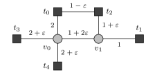
(a) Complete instance graph $G$. Invisible edges have distance costs.

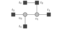
(b) Minimum solution with cost $8+4\varepsilon$.

(c) Minimum Voronoi-based solution with cost $9+3\varepsilon$.

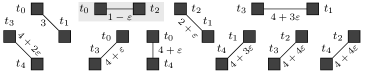
(d) All $2$-components and their costs.

(e) All $4$-components that can be constructed with and without using Voronoi regions.

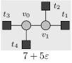
(f) The $4$-components that cannot be constructed using Voronoi regions.

(g) The latter $4$-components constructed using Voronoi regions.

Figure 3: Fig. 3(a) shows the complete instance $G$. The costs of the invisible edges coincide with the distances between each node pair. The unique Voronoi regions are $\mathcal{V}(t_{i})=\{t_{i},v_{i}\}$ for $i\in\{0,1\}$ and $\mathcal{V}(t_{j})=\{t_{j}\}$ for $j\in\{2,3,4\}$. By the structure of the instance, a minimum $4$-restricted Steiner tree contains a $4$-component and a $2$-component, i.e., $3$-components are not beneficial. Fig. 3(b) shows the minimum $4$-restricted Steiner tree that is obtained by an enumeration of full components. Fig. 3(c) shows the minimum $4$-restricted Steiner tree that is obtained by full components that are constructed from Voronoi regions only. The tree in Fig. 3(b) is constructed from the full components shown in Figures 3(d), 3(e) and 3(f) whereas the tree in Fig. 3(c) uses Fig. 3(g) instead of 3(f). The full components used in Fig. 3(b) and 3(c) are marked.

The question arises whether such a construction always leads to a set of full components that is necessary to obtain a minimum $k$-restricted Steiner tree. Zelikovsky [1993b] showed that GCF with $k=3$ and $\textit{win}_{\text{abs}}$ finds the same maximum win in each iteration no matter if gen=all or gen=voronoi is used. An analogous argumentation can be applied to prove this for $\textit{win}_{\text{rel}}$. We generalize this result to see that Voronoi regions can always be used for $k=3$. The following lemma shows that a minimum $3$-restricted Steiner tree can be obtained even if $\mathcal{C}_{3}$ is generated using Voronoi regions.

Lemma 2.

Let $T$ be a $3$-restricted Steiner tree for $\bar{G}$. There is a $3$-restricted Steiner tree $T^{\ast}$ for $\bar{G}$ with $d(T^{\ast})\leq d(T)$ such that for each nonterminal $v_{C}$ in any full component $C$ in $T^{\ast}$, we have $v_{C}\in\mathcal{V}(R_{C})$.

Proof.

As $T$ is $3$-restricted, we can w.l.o.g. assume that no nonterminal in $T$ is adjacent to another nonterminal. Hence there is at most one nonterminal in each full component. On the other hand, any $3$-component $C$ has at least one nonterminal. Let $v_{C}$ be the unique nonterminal in $C$. If $v_{C}\in\mathcal{V}(R_{C})$ for each $3$-component $C$, we are done.

Let $C$ be a $3$-component with $v_{C}\notin\mathcal{V}(R_{C})$. There must be a terminal $s\in R\setminus R_{C}$ such that $v_{C}\in\mathcal{V}(s)$. Consider the three connected components that emerge by removing $v_{C}$ from $T$. Let $t$ be the unique terminal adjacent to $v_{C}$ that is in the same connected component as $s$. Replacing edge $\{v_{C},t\}$ by $\{v_{C},s\}$ in the original $T$ results in a tree $T^{\prime}$ with $d(T^{\prime})\leq d(T)$. We obtain $T^{\ast}$ by repeating this process. ∎

The proof does not generalize to $k\geq 4$: let $u,v\in V_{C}\setminus{R_{C}},v\notin\mathcal{V}(R_{C})$; replacing an edge can remove $\{v,t\}$ and insert $\{u,s\}$ instead of $\{v,s\}$. That way, it is possible that the cost of the resulting component increases. For example, the $4$-component of Fig. 3(b) would become the $4$-component of Fig. 3(c). Fig. 3 leads to the following observation.

Observation 3.

For $k\geq 4$, the Voronoi-based approach does not guarantee minimum $k$-restricted Steiner trees. Even for $k=4$, one can obtain solutions at least $9/8$ times worse than using full component enumeration.

Direct generation of $3$-restricted components (gen=ondemand).

This way of generating full components has been proposed by Zelikovsky [1993a]. It is only available for $3$-restricted components and $\textit{win}_{\text{abs}}$ in the Greedy Contraction Framework.

In contrast to the other generation strategies, there is no explicit generation phase. An optimal full component is directly constructed when necessary. Therefore, we iterate over all nonterminals $v\in V\setminus R$. In each iteration, we

1. find $s_{0}\in R$ with minimum distance $d(v,s_{0})$ to $v$,

2. find $s_{1}\in R\setminus\{s_{0}\}$ with maximum $d(\textit{save}_{M}(s_{0},s_{1}))-d(v,s_{1})$,

3. find $s_{2}\in R\setminus\{s_{0},s_{1}\}$ with maximum $\textit{win}_{\text{abs}}(M,C)=\textit{save}(M,C)-d(v,s_{0})-d(v,s_{1})-d(v,s_{2})$ where $C$ is the full component of terminals $s_{0},s_{1},s_{2}$ with center $v$,

and keep the full component $C$ with maximum $\textit{win}_{\text{abs}}(M,C)$.

3.2 Greedy Contraction Framework

Reduction of the full component set.

We can show that the win of any $C\in\mathcal{C}_{k}$ will never increase during the execution of GCF or LCA. This follows from $\textit{save}(M,C_{2})\geq\textit{save}(M/C_{1},C_{2})$ and $\textit{save}(M,C_{2})\geq\textit{save}(M/\textit{Loss}(C_{1}),C_{2})$ for any full components $C_{1},C_{2}$, which we prove in the following lemma.

Lemma 4.

Consider the metric complete graph $M$ in any iteration of GCF or LCA. Let $u,v\in R$ with $u\neq v$, edge $e=\{u,v\}$ with arbitrary cost $d(e)$, and $M_{e}:=(V_{M},E_{M}\cup\{e\})$. We have $\textit{save}(M,C)\geq\textit{save}(M_{e},C)$.

Proof.

Consider $\textrm{MST}(M)$. Inserting edge $e$ closes a cycle, so either $e$ or $f:=\textit{save}_{M}(u,v)$ will not be in $\textrm{MST}(M_{e})$. We have $d(\textrm{MST}(M_{e}))=d(\textrm{MST}(M))+\min\{0,d(e)-d(f)\}$, and thus

$$\textit{save}(M,C)-\textit{save}(M_{e},C)$$

$$=d(\textrm{MST}(M))-d(\textrm{MST}(M/C))-d(\textrm{MST}(M_{e}))+d(\textrm{MST}(M_{e}/C))$$

$$=d(\textrm{MST}(M_{e}/C))-d(\textrm{MST}(M/C))-\min\{0,d(e)-d(f)\}$$

which proves the claim if $d(\textrm{MST}(M_{e}/C))\geq d(\textrm{MST}(M/C))$.

If $d(e)>d(f)$, we have $\textrm{MST}(M_{e})=\textrm{MST}(M)$. Now consider $d(e)\leq d(f)$. For any $x,y\in R_{C}$ with $\textit{save}_{M}(x,y)=f$, we have $d(\textit{save}_{M_{e}}(x,y))\leq d(f)$. In any case, we have $d(\textrm{MST}(M_{e}/C))\geq d(\textrm{MST}(M/C))$ and thus the claim holds. ∎

We can utilize this fact to reduce the number of full components. Every time we find a non-promising full component, we remove that full component from $\mathcal{C}_{k}$. In particular, when we construct a non-promising full component, we discard it already before inserting it into $\mathcal{C}_{k}$. We denote this variant by reduce=on. Note that this variant does not work together with gen=ondemand.

Save computation.

In order to compute the win of a full component $C$, we first have to compute $\textit{save}(M,C)=d(\textrm{MST}(M))-d(\textrm{MST}(M/C))$. Doing a contraction and MST computation for each potential component would be cumbersome and inefficient.

Since we can consider a contraction of $u$ and $v$ as an insertion of zero-cost edges $\{u,v\}$, we can construct $\textrm{MST}(M/C)$ from $\textrm{MST}(M)$ by removing $\textit{save}_{M}(u,v)$ and inserting a zero-cost edge $\{u,v\}$ for each pair $u,v\in R_{C}$. It follows that $\textit{save}(M,C)$ coincides with the total cost of the removed save edges. If we are able to compute $\textit{save}_{M}(u,v)$ in, say, constant time, we are also able to compute $\textit{save}(M,C)$ in $\mathcal{O}\!\left(k\right)$.

One simple idea (also proposed by Zelikovsky [1993b]) is to build and use an $|R|\times|R|$ matrix to simply lookup the most expensive edges between each pair of terminals directly. After each change of $M$, this matrix is (re-)built in time $O(|R|^{2})$. We call this method save=matrix.

The build times of the former approach can be rather expensive. Zelikovsky [1993a] provided another approach that builds an auxiliary binary arborescence $W(T)$ for a given tree $T:=\textrm{MST}(M)$. The idea of $W(T)$ is to represent a cost hierarchy to find a save edge using lowest common ancestor queries. We define $W(T)$ inductively:

• If $T$ is only one node $v$, $W(T)$ is a single node representing $v$.

• If $T$ is a tree with at least one edge, the root node $r$ of $W(T)$ represents the maximum-cost edge $e$ of $T$. By removing $e$, $T$ decomposes into two trees $T_{1}$ and $T_{2}$. The roots of $W(T_{1})$ and $W(T_{2})$ are the children of $r$ in $W(T)$.

Nodes in $T$ are leaves in $W(T)$ and edges in $T$ are inner nodes in $W(T)$. To construct $W(T)$, we first sort the edges by their costs and then build $W(T)$ bottom-up. The construction time of $W(T)$, dominated by sorting, takes time $\mathcal{O}\!\left(|R|\log|R|\right)$.

We now want to perform lowest common ancestor queries on $W(T)$ in $\mathcal{O}\!\left(1\right)$ time. Let $n\in\mathcal{O}\!\left(|R|\right)$ be the number of nodes in $W(T)$. Some preprocessing is necessary to achieve that. The theoretically best known algorithm by Harel and Tarjan [1984] needs time $\mathcal{O}\!\left(n\right)$ for preprocessing but is too complicated and cumbersome to implement and use in practice. We hence use a simpler and more practical $\mathcal{O}\!\left(n\log n\right)$-algorithm by Bender and Farach-Colton [2000]. In either case, the time to build $W(T)$ and do the preprocessing is $\mathcal{O}\!\left(|R|\log|R|\right)$.

Instead of rebuilding $W(T)$ from scratch after a contraction, we can directly update $W(T)$ in time proportional to the height of $W(T)$. This can be accomplished by adding a zero-cost edge-representing node $u_{0}$, moving the contracted nodes $u_{1},u_{2}$ to be children of $u_{0}$, and then fixing $W(T)$ bottom-up from the former parents of $u_{1}$ and $u_{2}$ up to the root. On the way up, we remove the node that represents edge $\textit{save}_{M}(u_{1},u_{2})$ as soon as we see it.

We denote the variant of fully rebuilding $W(T)$ by save=static, and the variant of updating $W(T)$ by save=dynamic. In the latter case, it is sufficient to update $W(T)$ only, without necessity to store $M$ or $T$ explicitly.

Evaluation passes.

The original GCF needs $\mathcal{O}\!\left(|R|\right)$ passes in the evaluation phase. In each iteration, the whole (probably reduced) list $\mathcal{C}_{k}$ of full components has to be evaluated. We investigate another heuristic strategy that performs one pass and hence evaluates the win function of each full component at most twice. The idea is to sort $\mathcal{C}_{k}$ in decreasing order by their initial win values. Then we do one single pass over the sorted $\mathcal{C}_{k}$ and contract the promising full components. We call this strategy singlepass=on.

Lemma 5.

GCF with singlepass=on on $k$-restricted components has an approximation ratio smaller than $2$.

Proof.

Let $T$ be the Steiner tree solution of the MST-based $2$-approximation [Kou et al. 1981] and $T^{\ast}$ be a minimum Steiner tree. Consider the case that there are promising $k$-restricted components. At least one of them, say $C$, will be chosen and contracted in the single pass. This yields a Steiner tree $T^{\prime}$ with $d(T^{\prime})\leq d(T)-\textit{win}_{\text{abs}}(T,C)<2d(T^{\ast})$. Now consider the case that there are no promising $k$-restricted components. The algorithm would not find any full component to contract, but GCF with singlepass=off would also not contract any full component. By the approximation ratio of GCF, we have $d(T)<2d(T^{\ast})$. ∎

3.3 Algorithms Based on Linear Programming

We now consider variants for the LP-based algorithm.

Solving the LP relaxation.

First, we can observe that during separation, each full component’s inner structure is irrelevant for the max-flow computation. It hence suffices to insert a directed star into $N$ for each chosen full component. That way, the size of $N$ becomes independent of $|V|$; this should hence be particularly beneficial if $|R|$ is small compared to $|V|$.

To solve SER, we start with constraints (3a). Since we need (4) for the separation algorithm, we may include them in the initial LP formulation (denoted by presep=initial) or add them iteratively when needed (presep=ondemand).

In the beginning of the separation process, it is likely that the hypergraph $(R,\mathcal{\bar{C}}_{k})$ for a current solution $\bar{x}$ is not connected. Hence it may be beneficial to apply a simpler separation strategy first: perform a connectivity tests and add (3b) for each full component. This variant is denoted by consep=on.

Pruning full leaf components.

After solving the LP relaxation, the actual approximation algorithm with multiple minimum-cost flow computations in a changing auxiliary network starts. However, solution $\bar{x}$ is not always fractional. If the solution is fractional, there may still be full components $C$ with $\bar{x}_{C}=1$. We will show that we can directly choose some of these integral components for our final Steiner tree and then generate a smaller network $N$ that does not contain them.

Lemma 6.

Let $C^{\ast}\in\mathcal{\bar{C}}_{k}$ and $|R_{C^{\ast}}\cap\bigcup_{C\in\mathcal{\bar{C}}_{k}\setminus\{C^{\ast}\}}{R_{C}}|=1$. Let $v^{\ast}$ be that one terminal. The solution $\bar{x}$ obtained by setting $\bar{x}_{C^{\ast}}:=0$ is feasible for the same instance with reduced terminal set $R\setminus(R_{C^{\ast}}\setminus\{v^{\ast}\})$.

Proof.

By constraint (4) we have $\bar{x}_{C^{\ast}}=1$. We set $\bar{x}_{C^{\ast}}:=0$ and $R:=R\setminus(R_{C^{\ast}}\setminus\{v^{\ast}\})$, and observe how the left- (LHS) and the right-hand side (RHS) of the SER constraints change. The LHS of constraint (3a) is decreased by $(|R_{C^{\ast}}|-1)x_{C^{\ast}}=|R_{C^{\ast}}|-1$, its RHS is decreased by $|R_{C^{\ast}}\setminus\{v^{\ast}\}|=|R_{C^{\ast}}|-1$; constraint (3a) still holds. Consider (3b). On the LHS, the $\bar{x}_{C}$-coefficients of full components $C\neq C^{\ast}$ with $\bar{x}_{C}>0$ are not affected since $R^{\prime}\cap R_{C}$ contains no terminal from $R_{C^{\ast}}\setminus\{v^{\ast}\}$. The LHS hence changes by $\max(|R^{\prime}\cap R_{C^{\ast}}|-1,0)$. The RHS is decreased by $|R^{\prime}\cap(R_{C^{\ast}}\setminus\{v^{\ast}\})|$ which coincides with the LHS change. ∎

Hence, we can always choose and contract such full leaf components without removing any core edges from outside that component and without expensive search. We call this strategy prune=on.

Solving a stronger LP relaxation.

One way that could help to improve the solution quality is to use a strictly stronger relaxation than SER. Consider the constraints

$$\sum_{C\in\mathcal{C}^{\prime}}{x_{C}}\;\leq\;S(\mathcal{C}^{\prime})\qquad\forall\mathcal{C}^{\prime}\subseteq\mathcal{C}_{k},$$ (5)

where $S(\mathcal{C}^{\prime})$ is the maximum number of full components of $\mathcal{C}^{\prime}$ that can simultaneously be in a valid solution. $S(\mathcal{C}^{\prime})$ coincides with the maximum number of hyperedges that can form a subhyperforest in $H=(R,\{{R_{C}}\,\mid\,{C\in\mathcal{C}^{\prime}}\})$. Unfortunately, obtaining $S(\mathcal{C}^{\prime})$ is an NP-hard problem as can be shown by an easy reduction from Independent Set.

We try to solve the problem for a special case of $\mathcal{C}^{\prime}$ only:

$$\sum_{C\in\mathcal{C}^{\prime}}{x_{C}}\; \leq\;1 \forall\mathcal{C}^{\prime}\subseteq\mathcal{C}_{k}\colon|C_{i}\cap C_{j}|\geq 2\;\forall C_{i},C_{j}\in\mathcal{C}^{\prime}\text{.}$$ (6)

Lemma 7.

SER with constraint (6) is strictly stronger than SER.

Proof.

Clearly, the new LP is at least as strong as SER since we only add constraints. Let $G=(V,E)$ be a graph with $V=\{v_{0},\ldots,v_{k},t_{0},\ldots,t_{k}\}$ and $E=\{{\{v_{i},t_{i}\},\{v_{i},v_{i+1}\}}\,\mid\,{i=0,\ldots,k}\},v_{k+1}=v_{0}$, with terminals $R=\{t_{0},\ldots,t_{k}\}$, cost $1$ for all edges incident to any terminal, and cost $0$ for all other edges. Each full component $C$ has exactly cost $|R_{C}|$.

Consider the solution $\bar{x}$ with

$$\bar{x}_{C}=\begin{cases}\frac{k}{k^{2}-1}&\text{if $|R_{C}|=k$,}\\ 0&\text{otherwise}\end{cases}$$

that is feasible to SER by

$$\sum_{C\in\mathcal{C}_{k}}{(|R_{C}|-1)\bar{x}_{C}} \;=\;\sum_{C\in\mathcal{C}_{k}\colon|R_{C}|=k}{(k-1)\frac{k}{k^{2}-1}}$$

$$\;=\;(k+1)(k-1)\frac{k}{k^{2}-1}\;=\;k\;=\;|R|-1\text{,}$$

and (3b) holds since for $|R^{\prime}|=k$ we have $\frac{k}{k^{2}-1}\leq k-1$, and for $|R^{\prime}|<k$ we have $0\leq|R^{\prime}|-1$. The objective value for $\bar{x}$ is $\sum_{C\in\mathcal{C}_{k}}{|R_{C}|\bar{x}_{C}}=(k+1)k\frac{k}{k^{2}-1}=\frac{k^{3}+k^{2}}{k^{2}-1}$.

Let $\bar{X}_{\ell}:=\sum_{C\in\mathcal{C}_{k}\colon|R_{C}|=\ell}{\bar{x}_{C}}$. Note that for any solution $\bar{x}$, (3a) and the objective function can be written as $\sum_{\ell=2}^{k}{(\ell-1)\bar{X}_{\ell}}=k$ and $\sum_{\ell=2}^{k}{\ell\bar{X}_{\ell}}$, respectively. Assume we decrease $\bar{X}_{k}$ by some $\varepsilon>0$. Since $\sum_{\ell=2}^{k}{(\ell-1)\bar{X}_{\ell}}=k-(k-1)\varepsilon<k=|R|-1$, we would have to increase $\bar{X}_{i}$ by $\frac{k-1}{i-1}\varepsilon_{i}$ for all $i\in\{2,\ldots,k-1\}$ to become feasible for (3a) again. Here, $\varepsilon_{2},\ldots,\varepsilon_{k-1}>0$ are chosen such that they sum up to $\varepsilon$. This increases the objective value by $\sum_{i=2}^{k-1}{i\,\frac{k-1}{i-1}\varepsilon_{i}}-k\varepsilon$ which is clearly minimized by setting $\varepsilon_{k-1}:=\varepsilon$ and $\varepsilon_{i}:=0$ for $i<k-1$. The increase of the objective value is hence at least $(k-1)\frac{k-1}{k-2}\varepsilon-k\varepsilon=\frac{1}{k-2}\varepsilon>0$.

Since

$$\sum_{C\in\mathcal{C}_{k}}{\bar{x}_{C}} \;=\;(k+1)\frac{k}{k^{2}-1}\;=\;\frac{k}{k-1}\;=\;1+\frac{1}{k-1}$$

violates (6), we add the constraint $\sum_{C\in\mathcal{C}_{k}\colon|R_{C}|=k}{x_{C}}\leq 1$. We thus have to decrease $\bar{X}_{k}$ by $\frac{1}{k-1}$ to form a feasible solution, which increases the objective value. ∎

Finding a $\mathcal{C}^{\prime}$ is equivalent to finding a clique in the conflict graph $G^{\prime}=(\mathcal{C}_{k},\{{\{C_{i},C_{j}\}}\,\mid\,{C_{i},C_{j}\in\mathcal{C}_{k},|R_{C_{i}}\cap R_{C_{j}}|\geq 2}\})$. Based on the proof of Lemma 7, we restrict ourselves to cliques with at most $k+1$ nodes. Such cliques can be found in polynomial time for constant $k$, in order to separate the corresponding constraints. Observe that $G^{\prime}$ need only be constructed from $\mathcal{\bar{C}}_{k}$ instead of $\mathcal{C}_{k}$. We call this strategy stronger=on.

Bounding the LP relaxation.

An idea to improve the running time for the LP is to initially compute a simple $2$-approximation and apply its solution value as an upper bound on the objective value. If this bound is smaller than the pure LP solution, there is no feasible solution to the bounded LP and we simply take the $2$-approximation. We call this strategy bound=on.

4 Experimental Evaluation

In the following experimental evaluation, we use an Intel Xeon E5-2430 v2, 2.50 GHz running Debian 8. The binaries are compiled in 64bit with g++ 4.9.0 and -O3 optimization flag. All algorithms are implemented as part of the free C++ Open Graph Drawing Framework (OGDF), the used LP solver is CPLEX 12.6. We evaluate our algorithms with the 1 200 connected instances from the SteinLib library [Koch et al. 2000], the currently most widely used benchmark set for STP.

We say that an algorithm fails for a specific instance if it exceeds one hour of computation time or needs more than 16 GB of memory. Otherwise it succeeds. Success rates and failure rates are the percentage of instances that succeed or fail, respectively.

We evaluate the solution quality of a solved instance by computing a gap as $\frac{d(T)}{d(T^{\ast})}-1$, the relative discrepancy between the cost of the found tree $T$ and the cost of the optimal Steiner tree $T^{\ast}$, usually given in thousandths (‰). When no optimal solution values are known, we use the currently best known upper bounds from the 11th DIMACS Challenge [2014].

Table 1: Mapping from SteinLib instance groups to our instance grouping.

Group	SteinLib group
EuclidSparse	P6E
EuclidComplete	P4E
RandomSparse	B, C, D, E; P6Z; non-complete instances from MC
RandomComplete	P4Z; complete instances from MC
IncidenceSparse	non-complete instances from I080, I160, I320 and I640
IncidenceComplete	complete instances from I080, I160, I320 and I640
ConstructedSparse	PUC; SP
SimpleRectilinear	ES$\star$FST and TSPFST with $|R|<300$ or $|R|/|V|>0.75$
HardRectilinear	ES$\star$FST and TSPFST with $|R|\geq 300$ and $|R|/|V|\leq 0.75$
VLSI / Grid	ALUE, ALUT, LIN, TAQ, DIW, DMXA, GAP, MSM; 1R, 2R
WireRouting	WRP3, WRP4

Besides the original SteinLib instance groups, we also consider a slightly different grouping where suitable, to obtain fewer but internally more consistent graph classes, see Table 1 for details. Additionally, Large consists of all instances with more than 16 000 edges or 8 000 nodes, Difficult are instances that could not be solved to proven optimality within one hour (according to the information provided by SteinLib), and NonOpt are 35 instances (31 from PUC and 4 from I640) we still do not know the optimal values for. Last but not least, we grouped instances by terminal coverage: the group Coverage $X$ contains all instances with $X-10<100\,|R|/|V|\leq X$.

4.1 Evaluation of $2$-Approximations

We consider the basic $2$-approximations by Takahashi and Matsuyama [1980] (TM, with [Poggi de Aragão and Werneck 2002]), Kou et al. [1981] (KMB), and Mehlhorn [1988] (M). TM and M succeed for all instances, whereas KMB fails for eight instances (mainly from TSPFST) due to the memory limit. Every instance is solved in less than 0.1 seconds using M, less than 0.3 seconds using TM, and at most 52 seconds using KMB (instance alue7080).

Comparing the solution quality of TM, KMB, and M gives further insights. TM yields significantly better solutons than M: 80.3 % of the solutions are better using TM and only 1.7 % are worse. Especially wire-routing instances are solved much better using TM. For example, the optimal solution for wrp3-60 is 6 001 164, and it is solved to 6 001 175 (gap 0.0018 ‰) using TM and to 11 600 427 (gap 933.03 ‰, i.e., almost factor $2$) using M. A comparison between TM and KMB gives similar results. On average, gaps are 74.1 ‰ for TM, 194.5 ‰ for M, and 198.3 ‰ for KMB. TM solves 9.2 % of the instances to optimality; M only 3.9 % and KMB 3.8 %.

We see that TM is the best candidate: although slower than M, it takes only negligible time, and solution quality is almost always better than for M or KMB. When considering $2$-approximations in the following, we will always choose TM. In particular, we set TM to be the final $2$-approximation to incorporate contracted full components (see Section 2.1).

4.2 Evaluation of Full Component Enumeration

Shortest path algorithms.

Before we consider the enumeration of full components, we compare the running times to compute the shortest path matrices using sp=forbid and sp=prefer. In combination with dist=sssp, these running times differ by at most 0.5 seconds for 97.8 % of the instances. The only four outliers with more than 10 seconds time difference (maximum 120 seconds) are precisely the instances with a terminal coverage $|R|/|V|\geq 0.25$ and more than 8 000 nodes. In combination with dist=apsp, there are already 20 instances where forbid can save between 15 seconds and 6 minutes, but the differences are still negligible for 87.1 % of the instances. Hence, for the majority of the instances, forbid does not provide a significant time saving.

In contrast to this, we are more interested in the number of valid shortest paths that are obtained by the different variants. A smaller (but sufficient) set of valid paths results in fewer full components. On average, forbid generates a path between 76.3 % of all terminals pairs; prefer only between 59.1 %. In particular, forbid could not reduce the number of valid paths at all for 65.8 % of the instances. This number drops to 37.6 % using prefer, which is much better. Consequently, prefer yields 10.5 % fewer $3$-restricted components than sp=forbid. Since this saves memory and time for the further steps of the algorithm, we use sp=prefer in the following.

For $k=3$, we can either use dist=sssp or dist=apsp. While sssp is able to compute the shortest path matrices for every instance of the SteinLib, all instances with more than 15 000 nodes fail using apsp since the full APSP matrix is too big to fit into 16 GB of memory.

After filtering out all instances with negligible running times using both algorithms, we obtain the following rule of thumb: use sssp iff the graph is not too dense (say, density $E/\binom{|V|}{2}\leq 0.25$). There are only a handful of outliers (in the I640 set) with small differences of up to $0.2$ seconds. We hence apply this rule to our experiments.

Full component generation.

Fig. 4 shows the percentage of instances such that the $3$-restricted components can be generated in a given time, for each gen- and sp-variant. Note that gen=all:smart and gen=all:naïve use the same observation for $k=3$ and are hence equal. It can clearly be observed that gen=voronoi with sp=prefer (as said above) is the best choice for $k=3$.

Fig. 5 shows the success rates for the generation of $k$-restricted components for $k\in\{3,4,5,6\}$. We can see that gen=all:dw is superior for $k\geq 4$.

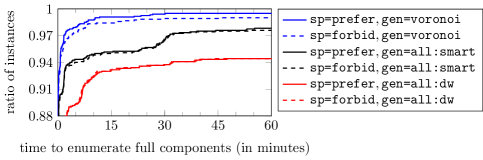
Figure 4: Percentage of instances whose $3$-restricted components are generated within the given time for different variants.

4.3 Evaluation of GCF and LCA

We now consider the strong combinatorial algorithms with $k=3$. Three instances failed for all algorithmic variants: rl11849fst (with 13 963 nodes and 11 849 terminals) is the only instance that failed due to the memory limit; es10000fst01 and fnl4461fst failed due to the time limit.

Strategies for GCF.

We first have a look at the reduction strategy reduce=on. A comparison for $\textit{win}_{\text{abs}}$ with gen=voronoi shows that without reduction, we generate 68 270 $3$-components on average, whereas we generate only 6 136 $3$-components with reduction; in other words, 91.0 % of the generated full components are not promising and are hence removed directly after construction. Considering the actual contractions, we effectively use 7.5 % of the generated unreduced full component set but 22.2 % of the reduced set. The biggest time savings can be observed on rectilinear instances, e.g., approximately half an hour for fl3795fst. Since reduce=on offers benefits without introducing overhead, it will always be enabled in the following.

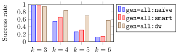
Figure 5: Success rates of component enumeration methods gen=all.

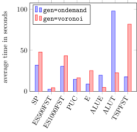
(a) Comparison between gen=ondemand and voronoi, each with save=static.

(b) Comparison between save strategies, each with $\textit{win}_{\text{rel}}$ and gen=voronoi.

Figure 6: Running times of GCF for different strategies, grouped by SteinLib instance groups, averaged over the instances where all considered strategies succeed. Different choices of secondary strategies show similar tendencies. Omitted instance groups have negligible running times.

However, gen=voronoi is not the only way to generate full components for $\textit{win}_{\text{abs}}$ and $k=3$. We can also use gen=ondemand. This strategy is often but not always beneficial in comparison to gen=voronoi. Let us, for example, consider GCF with $\textit{win}_{\text{abs}}$ and save=static. (Numbers for other choices of save are similar.) The average computation time decreases from 7.2 to 2.5 seconds. However, extreme examples where one or the other choice is better, are alut2625 with 192 seconds for voronoi and 849 seconds for ondemand, and fl3795fst with 1 782 and 148 seconds, respectively. See Fig. 6(a) for a comparison by instance groups. In general we might prefer ondemand but voronoi is the better choice for VLSI instances (like ALUE, ALUT and LIN).

We now compare the different strategies to compute save. Averaged over all instances, the times for save=static and save=dynamic are nearly the same. Strategy save=static is never (significantly) worse than save=matrix: the average time decreases from 10.3 (matrix) to 8.6 seconds (static) for gen=voronoi (and from 6.6 to 4.2 seconds for gen=ondemand). See Fig. 6(b) for a more detailed view based on SteinLib instance groups. Since static is easier to implement than dynamic, we recommend to use save=static.

Surprisingly, the strategy singlepass=on does not lead to notable time improvements in comparison to the original algorithm. The solution becomes worse in 33.3 % (28.4 %) and better in 22.7 % (18.8 %) of the instances using $\textit{win}_{\text{abs}}$ ($\textit{win}_{\text{rel}}$, respectively), deteriorating the solutions by 0.13 ‰ (0.28 ‰) on average. Hence, we will not consider singlepass=on in the following.

Table 2: Comparison of combinatorial algorithms by instance groups. Per group, we give the total number of instances (‘#’), portion of optimally solved instances, average gaps, and average solution times.

		Optimals%					Average gap‰					Average time in sec
Group	#	TM	ACO	AC3	RC3	LC3	TM	ACO	AC3	RC3	LC3	TM	ACO	AC3	RC3	LC3
EuclidSparse	15	33.3	93.3	86.7	80.0	66.7	15.18	1.92	1.99	2.00	5.27	0.00	0.00	0.00	0.00	0.00
EuclidComplete	14	7.1	78.6	78.6	78.6	78.6	10.84	0.35	0.35	0.35	0.35	0.01	0.08	0.08	0.08	3.98
RandomSparse	96	27.1	41.7	40.6	43.8	40.6	23.72	12.32	12.33	10.93	18.10	0.01	1.96	5.55	5.50	24.63
RandomComplete	13	30.8	61.5	61.5	61.5	53.8	22.34	20.55	37.56	39.73	45.03	0.00	0.01	0.01	0.01	0.06
IncidenceSparse	320	3.8	4.4	4.4	5.1	3.5	124.13	70.66	70.04	68.94	75.16	0.00	0.05	0.03	0.03	1.91
IncidenceComplete	80	0.0	0.0	0.0	0.0	0.0	384.29	126.37	127.30	128.71	126.65	0.06	0.26	0.28	0.29	40.90
ConstructedSparse	58	25.9	25.9	22.2	22.2	25.9	95.52	129.91	148.82	150.74	137.96	0.00	17.02	20.85	20.96	73.93
SimpleRectilinear	218	11.5	17.4	18.3	17.9	15.6	16.96	6.63	6.40	6.23	9.91	0.00	0.87	16.00	16.03	17.76
HardRectilinear	54	0.0	0.0	0.0	0.0	0.0	22.86	8.58	8.47	8.05	13.37	0.00	30.27	59.82	59.83	58.10
VLSI / Grid	207	10.6	35.7	35.3	33.8	29.0	33.83	9.75	9.94	9.74	24.17	0.00	5.99	1.53	1.53	2.12
WireRouting	125	3.2	4.0	2.4	3.2	3.2	0.01	0.01	0.01	0.01	0.02	0.00	0.14	0.07	0.07	0.60
Large	187	1.8	5.4	5.4	6.0	6.0	230.86	95.58	98.43	98.29	100.04	0.04	13.79	10.72	10.72	58.83
Difficult	146	2.7	2.7	1.8	2.7	3.6	206.46	110.13	116.83	117.39	113.30	0.03	7.55	8.89	8.94	60.16
NonOpt	35	—	—	—	—	—	134.88	153.86	169.94	170.53	156.79	0.01	20.95	23.61	23.74	112.92
Coverage 10	588	9.2	19.9	19.6	19.9	16.4	73.05	38.69	39.11	38.05	46.97	0.01	2.18	0.59	0.59	1.18
Coverage 20	159	9.6	18.5	16.4	15.8	14.4	111.47	57.03	57.89	59.16	61.03	0.00	1.13	0.40	0.40	22.89
Coverage 30	127	2.4	4.1	4.1	4.1	5.7	186.25	67.17	67.62	68.17	69.12	0.02	2.22	1.94	1.93	37.80
Coverage 40	92	1.1	3.3	3.3	3.3	2.2	26.19	9.55	9.27	8.82	15.60	0.00	5.94	8.51	8.52	8.19
Coverage 50	135	5.5	18.1	18.1	18.9	16.5	23.80	27.40	32.54	32.82	30.03	0.00	5.04	9.23	9.23	13.36
Coverage 60	45	11.1	26.7	31.1	24.4	24.4	18.88	16.27	17.64	18.33	18.31	0.00	20.49	36.58	36.66	36.08
Coverage 70	18	44.4	50.0	44.4	44.4	38.9	6.37	1.98	2.44	2.14	3.76	0.00	4.91	24.19	24.07	23.32
Coverage 80	11	54.5	54.5	54.5	54.5	54.5	5.12	2.36	2.32	2.43	2.45	0.00	21.36	222.85	223.27	259.47
Coverage 90	14	21.4	28.6	28.6	35.7	42.9	3.87	0.70	0.78	0.69	0.68	0.00	0.99	23.76	23.69	23.09
Coverage 100	11	54.5	63.6	63.6	72.7	63.6	0.94	0.07	0.25	0.27	0.23	0.00	0.93	116.49	116.70	112.91
All	1200	9.1	18.1	17.8	17.9	15.7	76.06	38.23	39.22	38.95	43.91	0.01	3.54	7.24	7.24	15.02

Comparison.

We compare the following algorithms for $k=3$: GCF with $\textit{win}_{\texttt{abs}}$ and gen=voronoi (AC3), GCF with $\textit{win}_{\texttt{abs}}$ and gen=ondemand (ACO), GCF with $\textit{win}_{\texttt{rel}}$ (RC3), and LCA with $\textit{win}_{\texttt{loss}}$ (LC3). Later we will also consider AC$k$, RC$k$, and LC$k$ for $k\geq 4$ where gen=all:dw will be used. Success rates are 99.7 % for ACO and 99.5 % for AC3, RC3, and LC3. We observe that these success rates are clearly dominated by the full component generation method. See Table 2 for a comparison of solution quality and time consumption based on our instance groups. With respect to solution quality, all algorithms are worthwile: in comparison to TM, the average gap halves and the number of optimally solved instances doubles. Noteworthy exceptions are RandomComplete where only ACO provides (slightly) better average gaps than TM, and ConstructedSparse, where TM provides the best average gaps.

Among the strong algorithms ACO, AC3, RC3, and LC3, there is no clear winner regarding solution quality for a majority of the instances. RC3 is better than AC3 on average within almost identical running time. ACO is almost always better than AC3; if not, it is only slightly worse. We emphasize that ACO becomes—in comparison—significantly faster for increasing terminal coverage, and outperforms the other algorithms already for $|R|/|V|>0.2$. Although LC3 takes significantly more time than the other algorithms, the obtained solution quality is not significantly better. ACO offers the best compromise between time and solution quality.

4.4 Evaluation of the LP-based Algorithm

The main stages of the LP-based algorithm are (1) the full component enumeration, (2) solving the LP relaxation, and (3) the approximation based on the fractional LP solution. We have already evaluated the strategies for (1) in Section 4.2, and will now evaluate the different strategies for the remaining stages, for $k=3$.

Solving the LP relaxation.

Fig. 7 shows that consep=on is clearly beneficial. Together with presep=ondemand, it allows us to compute the LP solutions for 89.0 % of the instances; a slight improvement over the 88.9 % with presep=initial. We hence perform all further experiments using connectivity tests and by separating constraints (4).

Figure 7: Percentage of instances whose LP relaxations for $k=3$ are solved within the given time for different variants.

Strategies.

Using the original algorithm, all instances that pass stage (2) also pass stage (3) of the algorithm. That leads to the assumption that stages (1) and (2) are the dominating stages.

The distribution of time in the three stages is very different for different instances. We consider the 133 instances with more than 10 seconds computation time. On average, we spend 8.7 % of the time in (1), 90.4 % in (2) and 0.8 % in (3). Stage (1) dominates in 7.5 % of the instances. An extreme example is u2152fst where the algorithm spends 280 seconds in (1), 40 seconds in (2), and 85 seconds in (3). In the remaining 92.5 % of the instances, stage (2) dominates. There are many instances, especially in the *FST set, with a long running time in (2) but negliglible running times for (1) and (3); the most extreme example is linhp318fst spending 57 minutes in (2). Stage (3) never dominates. The most extreme example is d2103fst, where it spends 4 minutes in (1), 36 minutes in (2) and almost 2 minutes in (3). This means that—as for the previous combinatorial algorithms—the actual approximation algorithm needs the least of the whole running time.

The strategy prune=on achieves that the time of stage (3) becomes negligible for every instance. Although the overall effect of that strategy may be considered rather limited (since usually most of the time is not spent in the last stage anyhow), we apply this strategy in the following.

Table 3: Comparison of algorithms by instance groups. Per group, we give the total number of instances (‘#’), success rates, portion of optimally solved instances, average gaps, portion of instances where LP3 obtained a worse or equal solution than TM or ACO, and average solution times.

		Success%			Optimals%			Average gap‰			LP3$\geq$		Avg. time in sec
Group	#	ACO	LP3	BC	TM	ACO	LP3	TM	ACO	LP3	TM	ACO	ACO	LP3	BC
EuclidSparse	15	100.0	100.0	100.0	33.3	93.3	80.0	15.18	1.92	3.31	33.3	93.3	0.00	0.02	0.29
EuclidComplete	14	100.0	100.0	92.9	7.1	78.6	78.6	10.84	0.35	0.35	7.1	100.0	0.01	0.12	21.29
RandomSparse	96	100.0	75.0	100.0	27.1	41.7	33.3	23.62	13.16	17.01	66.7	92.7	0.03	88.36	0.92
RandomComplete	13	100.0	100.0	100.0	30.8	61.5	46.2	22.34	20.55	37.14	76.9	100.0	0.01	0.36	6.78
IncidenceSparse	320	100.0	93.8	88.1	3.8	4.4	3.2	118.71	70.04	75.35	44.1	69.7	0.01	2.10	120.22
IncidenceComplete	80	100.0	93.8	81.2	0.0	0.0	0.0	378.80	125.72	140.93	6.2	85.0	0.14	0.61	129.74
ConstructedSparse	58	100.0	67.2	25.9	25.9	25.9	18.5	84.88	108.32	132.50	87.9	86.2	0.01	7.05	147.98
SimpleRectilinear	218	99.5	95.9	99.5	11.5	17.4	21.1	17.16	6.69	5.03	19.3	45.0	0.07	77.93	0.42
HardRectilinear	54	96.3	3.7	94.4	0.0	0.0	0.0	21.99	8.57	2.57	96.3	96.3	0.30	3321.97	5.88
VLSI / Grid	207	99.5	98.6	86.5	10.6	35.7	35.7	33.82	9.73	11.04	20.3	83.6	0.05	2.28	159.90
WireRouting	125	100.0	100.0	89.6	3.2	4.0	3.2	0.01	0.01	0.01	51.2	57.6	0.08	13.85	182.54
Large	187	97.9	78.6	51.3	1.8	5.4	4.8	241.62	93.49	101.69	31.0	85.6	0.18	2.34	292.48
Difficult	146	98.6	74.0	25.3	2.7	2.7	1.8	198.75	98.15	106.51	56.8	80.8	0.18	20.49	1192.83
NonOpt	35	100.0	42.9	0.0	—	—	—	115.58	141.40	159.32	88.6	85.7	—	—	—
Coverage 10	588	99.8	99.3	87.9	9.2	19.9	19.2	73.03	38.37	43.31	37.2	74.8	0.05	3.30	124.23
Coverage 20	159	100.0	91.2	84.9	9.6	18.5	11.6	112.95	55.65	62.30	47.2	78.6	0.03	12.07	104.40
Coverage 30	127	99.2	71.7	76.4	2.4	4.1	3.3	183.84	66.71	69.44	39.4	79.5	0.02	13.62	193.39
Coverage 40	92	98.9	65.2	98.9	1.1	3.3	4.3	26.70	9.76	7.78	35.9	55.4	0.04	81.67	0.86
Coverage 50	135	100.0	83.7	91.1	5.5	18.1	15.7	20.92	17.11	17.98	32.6	54.8	0.03	138.78	0.88
Coverage 60	45	100.0	82.2	93.3	11.1	26.7	31.1	11.57	6.17	6.42	37.8	66.7	0.00	52.41	1.94
Coverage 70	18	100.0	66.7	100.0	44.4	50.0	44.4	2.27	0.68	2.20	77.8	88.9	0.00	0.42	0.07
Coverage 80	11	100.0	72.7	90.9	54.5	54.5	54.5	2.22	0.55	0.38	81.8	81.8	0.03	50.70	0.07
Coverage 90	14	92.9	57.1	100.0	21.4	28.6	42.9	3.60	0.53	0.09	64.3	85.7	0.06	69.26	0.10
Coverage 100	11	100.0	90.9	100.0	54.5	63.6	90.9	0.94	0.07	0.00	63.6	72.7	0.93	486.39	0.17
All	1200	99.7	89.0	88.2	9.1	18.1	17.2	75.13	36.81	40.65	39.8	72.2	0.05	33.09	96.07

The strategy stronger=on might not be as worthwhile: the success rate drops to 88.8 %. However, 68.0 % of the solved LP relaxations are solved integrally with stronger=on whereas it is only 50.0 % for the original LP relaxation. Although this sounds promising, the final solution of the majority (74.2 %) of the instances does not change and the solution value increases (becomes worse) for 17.6 % of the instances. A harsh example is i160-043 where the fractional LP solution increases by $1.5$ but the integral approximation increases from 1 549 to 1 724. Only 8.2 % of the solutions improve. A good example is i080-003 where the fractional LP solution 1 902 increases to the (integral) LP solution 1 903 and yields an improvement from 1 807 to the optimum Steiner tree value 1 713. We mention these examples to conclude that the observed integrality gap of the relaxation’s solution seems secondary. The primary influence for the solution quality seems to be the actual choice of full components in the fractional solution, and the choice of core edges. We hence refrain from using stronger=on in the following and cannot recommend it.

We now evaluate bound=on. The success rate increases to 92.2 %. LP solving times improve for 43.1 % of the instances and deteriorate for 10.8 %, solutions improve for 49.5 % and deteriorate for 19.3 %. This behavior is due to the fact that the LP solver hits the bound on 67.8 % of the successful instances and then just returns the $2$-approximation. — Although bound=on is worthwhile in practice, we will not use it in the following comparison. It can be seen as an aggregation to combine two distinct methods, whereas in the following, we want to see a clearer picture on the differences between the various methods.

Comparison.

We compare the LP-based approximation algorithm (LP$k$) with $k=3$ to the recommended $2$-approximation TM, the $11/6$-approximation ACO, and an exact algorithm: BC, a highly-tuned branch-and-cut approach presented by Fischetti et al. [2014]. BC has been one of the winners of the DIMACS [2014]. It is based on an integer linear program that—using a branch-and-cut framework—is arguably much easier to implement than, e.g., the sophisticated strong approximation algorithms.

See Table 3 for a comparison based on our instance groups. In comparison to TM only, LP3 achieves a significantly better solution quality for most of the instances it can solve, and the average running times may be justifiable. However, the much simpler algorithm ACO is clearly better in terms of time and solution quality: its solutions are not worse than LP3 solutions in 72.2 % of the instances. BC fails for insignificantly more instances than LP3. The results suggest to use BC for rectilinear instances and instances with terminal coverage $|R|/|V|\geq 0.4$.

4.5 Higher $k$

Finally, we consider the strong approximation algorithms for higher $k$. see Table 4. The success rates for $k=6$ drop below 60 % which can be considered clearly impractical. Hence we compare the key performance indicators for the instances where AC$k$, RC$k$, LC$k$, and LP$k$ succeed for $k=3,4,5$. (Recall that ACO does not generalize to $k>3$.) All algorithms improve their solution qualities with increasing $k$. This is surprising for AC$k$ since it is only proven to be a $11/6$-approximation for any $k\geq 3$. On the other hand, $11/6$ is smaller than the theoretically proven bounds of the other algorithms for $k\leq 5$. AC$k$, RC$k$, and LP$k$ are comparable regarding their average gaps; only LC$k$ turns out to be worse than the others. RC$k$ always achieves the smallest gaps and also has the smallest or reasonable small running times. This is remarkable since, according to theoretical bounds, RC$k$ is the worst choice for $k\leq 18$. LP$k$ has the highest chances to find the optimum. However, if it fails to find the optimum, the solution is either quite weak (worse gaps than AC$k$ and RC$k$) or non-existent (worst success rates).

In Table 5, we give a more in-depth look at the solution qualities of the algorithms with $k=3$ and $k=4$ only, since $k=4$ still offers good success rates. Interestingly, for AC$k$, RC$k$, and LC$k$, the WireRouting and NonOpt solutions become slightly worse when we increase $k$ from $3$ to $4$ We can also see that the algorithms perform bad on high-coverage instances regarding success rates. However, if successful, the solution quality is good, e.g., LP4 is already a good choice for terminal coverage $|R|/|V|>0.3$.

Table 4: Comparison of strong approximation algorithms for higher $k$. Per $k$, we give the success rates for each algorithm, and then—limited to the 787 instances that could be solved by all algorithms with $k\in\{3,4,5\}$—the portion of optimally solved instances, the average gaps, and the average running time.

	Success%				Optimals%				Average gap‰				Average time in sec
Alg	AC$k$	RC$k$	LC$k$	LP$k$	AC$k$	RC$k$	LC$k$	LP$k$	AC$k$	RC$k$	LC$k$	LP$k$	AC$k$	RC$k$	LC$k$	LP$k$
$k=3$	99.5	99.5	99.5	89.0	23.8	23.5	20.7	22.6	38.99	38.57	44.92	43.08	0.02	0.02	0.08	0.16
$k=4$	85.2	85.2	85.2	77.2	29.1	29.9	24.0	38.2	26.63	25.89	34.16	26.90	9.77	9.97	9.73	10.60
$k=5$	70.8	70.8	70.6	65.7	30.6	32.1	24.9	46.3	20.41	19.42	30.22	20.75	131.07	128.24	129.08	130.89
$k=6$	57.4	57.4	57.2	54.3

5 Conclusion

We considered the strong approximation algorithms for the Steiner tree problem (STP) with an approximation ratio below 2. While there has been many theoretical advances over the last decades w.r.t. the approximation ratio, their practical applicability and strength has never been considered. In particular, all these algorithms use the tool of $k$-restricted components as a central ingredient to achieve astonishing approximation ratios for $k\to\infty$, while the runtime is exponentially dependent on $k$. The concept hence turned out to be a main stumbling block in real-world applications since they are both time- and memory-consuming. This paper is an attempt to show the importance of the research field algorithm engineering. Amongst other findings, we pinpoint further worthwhile research questions both from the theoretical and the practical point of view, and hope to increase the awareness for the necessity to complement high-level theoretical research with practical considerations, in order to ensure a certain degree of ‘groundedness’ of the theory.

Table 5: Comparison of solution qualities obtained by algorithms for $k=3$ and $k=4$. Per instance group, we give the number of instances (‘#’) that could be solved by all considered algorithms, portion of optimally solved instances, and average gaps.

			Optimals%								Average gap‰
Group	#	%	AC3	AC4	RC3	RC4	LC3	LC4	LP3	LP4	AC3	AC4	RC3	RC4	LC3	LC4	LP3	LP4
EuclidSparse	15	100	86.7	86.7	80.0	80.0	66.7	73.3	80.0	100	1.99	1.59	2.00	1.40	5.27	4.95	3.31	0.00
EuclidCompl.	13	92.9	84.6	100	84.6	100	84.6	100	84.6	100	0.36	0.00	0.36	0.00	0.36	0.00	0.36	0.00
Rand.Sparse	61	63.5	57.4	72.1	60.7	70.5	57.4	57.4	50.8	72.1	13.26	8.63	11.08	7.69	21.58	16.78	17.74	7.17
Rand.Compl.	12	92.3	66.7	58.3	66.7	50.0	58.3	66.7	50.0	66.7	26.20	22.66	28.55	19.70	35.19	27.24	26.64	23.12
Incid.Sparse	284	88.8	4.9	6.7	5.6	8.1	3.9	6.0	3.5	9.2	68.51	50.18	67.29	49.37	74.24	58.49	74.67	50.06
Incid.Compl.	71	88.8	0.0	0.0	0.0	0.0	0.0	0.0	0.0	0.0	125.76	78.01	127.43	77.56	125.53	77.52	140.58	95.26
Constr.Sparse	25	43.1	28.6	33.3	28.6	33.3	33.3	23.8	23.8	28.6	100.90	62.78	105.25	66.40	96.28	78.39	107.71	68.95
SimpleRect.	175	80.3	18.9	21.1	17.1	22.3	14.9	16.6	20.0	47.4	6.69	5.08	6.55	3.82	10.35	8.14	5.21	1.27
VLSI / Grid	180	87.0	40.6	52.2	38.9	53.3	33.3	42.2	41.1	67.2	9.36	5.17	9.06	4.39	23.22	20.29	10.56	2.49
WireRouting	91	72.8	3.3	5.5	4.4	6.6	4.4	3.3	4.4	6.6	0.01	0.02	0.01	0.02	0.02	0.02	0.01	0.01
Large	112	11.4	6.5	9.3	7.4	9.3	7.4	6.5	7.4	12.0	103.13	63.07	102.49	61.82	105.14	67.84	110.40	73.51
Difficult	63	43.2	3.4	5.1	5.1	5.1	6.8	1.7	3.4	5.1	112.14	75.27	112.47	75.30	111.28	79.14	115.25	80.67
NonOpt	4	59.9	—	—	—	—	—	—	—	—	94.28	107.82	96.42	108.43	103.94	114.57	101.74	94.45
Coverage 10	525	89.3	21.7	27.8	22.1	28.2	18.2	22.3	21.3	34.5	40.88	28.21	39.65	27.01	48.90	37.93	45.89	27.75
Coverage 20	129	81.1	18.6	19.4	17.8	21.7	16.3	16.3	13.2	22.5	52.14	36.72	53.80	37.64	55.55	42.71	58.16	41.33
Coverage 30	66	52.0	7.6	10.6	7.6	12.1	10.6	12.1	6.1	10.6	62.92	42.80	64.10	44.78	65.63	44.79	65.07	48.54
Coverage 40	52	56.5	5.8	9.6	5.8	7.7	3.8	3.8	7.7	21.2	9.23	6.51	8.86	5.34	15.70	11.71	7.59	2.01
Coverage 50	97	71.9	19.6	22.7	19.6	25.8	17.5	19.6	19.6	47.4	20.31	11.62	20.70	10.24	21.24	15.07	18.18	8.89
Coverage 60	35	77.8	40.0	40.0	31.4	37.1	31.4	31.4	40.0	77.1	3.39	4.44	4.39	3.11	4.04	2.85	2.06	0.58
Coverage 70	12	66.7	66.7	91.7	66.7	83.3	58.3	83.3	66.7	91.7	0.92	0.44	0.74	0.24	2.57	2.43	2.20	0.01
Coverage 80	6	54.5	100	100	100	100	100	100	100	100	0.00	0.00	0.00	0.00	0.00	0.00	0.00	0.00
Coverage 90	4	28.6	75.0	75.0	75.0	75.0	100	75.0	100	100	0.49	0.49	0.49	0.49	0.00	0.49	0.00	0.00
Coverage 100	1	9.1	100	100	100	100	100	100	100	100	0.00	0.00	0.00	0.00	0.00	0.00	0.00	0.00
All	927	77.2	21.2	25.9	21.0	26.5	18.5	21.3	20.4	34.9	37.67	25.89	37.35	25.22	43.39	32.99	41.15	25.99

For each strong approximation algorithm, we implemented the most promising variants, both of combinatorial and LP-based nature. Thereby, we identified several areas to improve or extend the known algorithms either theoretically (e.g., extending the applicability of the gen=voronoi strategy) or practically. We conducted a large study of the different algorithms and their variants, and compared them to simple $2$-approximations and an exact algorithm.

The choice of $k=3$ turns out to be practical; there, the simplest and oldest below-2 approximation—Zelikovsky’s $11/6$ approximation, combined with a direct $3$-restricted component generation [Zelikovsky 1993a]—offers the best compromise between time consumption and solution quality in practice. For higher $k$, the ‘relative greedy heuristic’ [Zelikovsky 1995] seems to be a viable choice w.r.t. solution quality. This is surprising since the loss-contracting algorithm [Robins and Zelikovsky 2005] and the LP-based algorithm [Goemans et al. 2012] provide better theoretical bounds.

In order to make the strong approximations more practical for higher $k$, it seems inevitable to find a way to significantly decrease the number of considered full components. This could, e.g., be achieved by a more efficient generation scheme (perhaps a generalization of the direct full component generation to $k\geq 4$), by removing dominated full components, or by starting with a small number of full components and constructing further ones only when it seems fit. All the above approaches clearly deserve further in-depth studies, both from theory and practice.

Acknowledgement.

We are grateful to Matthias Woste for initial implementations.

References

- [1]
- Aneja [1980] Y. P. Aneja. 1980. An Integer Linear Programming Approach to the Steiner Problem in Graphs. Networks 10, 2 (1980), 167–178.
- Bender and Farach-Colton [2000] M. A. Bender and M. Farach-Colton. 2000. The LCA Problem Revisited. In Proc. of LATIN 2000 (LNCS), Vol. 1776. Springer, 88–94.
- Berman and Ramaiyer [1994] P. Berman and V. Ramaiyer. 1994. Improved Approximations for the Steiner Tree Problem. Journal of Algorithms 17, 3 (1994), 381–408.
- Bern and Plassmann [1989] M. Bern and P. Plassmann. 1989. The Steiner Problem with Edge Lengths 1 and 2. Inform. Process. Lett. 32, 4 (1989), 171–176.
- Beyer and Chimani [2014] S. Beyer and M. Chimani. 2014. Steiner Tree 1.39-Approximation in Practice. In MEMICS 2014 (LNCS), Vol. 8934. 60–72.
- Borchers and Du [1995] A. Borchers and D.-Z. Du. 1995. The -Steiner ratio in graphs. In Proc. of STOC 1995. ACM, 641–649.
- Byrka et al. [2013] J. Byrka, F. Grandoni, T. Rothvoß, and L. Sanità. 2013. Steiner Tree Approximation via Iterative Randomized Rounding. J. ACM 60, 1 (2013), 6:1–33.
- Chakrabarty et al. [2010a] D. Chakrabarty, J. Könemann, and D. Pritchard. 2010a. Hypergraphic LP Relaxations for Steiner Trees. In Proc. of IPCO 2010 (LNCS), Vol. 6080. Springer, 383–396.