The hydrogen-poor superluminous supernova iPTF 13ajg and its host galaxy in absorption and emission

Abstract

We present imaging and spectroscopy of a hydrogen-poor superluminous supernova (SLSN) discovered by the intermediate Palomar Transient Factory: iPTF 13ajg. At a redshift of $z$=0.7403, derived from narrow absorption lines, iPTF 13ajg peaked at an absolute magnitude $M_{u,{\rm AB}}=-22.5$, one of the most luminous supernovae to date. The $uBgRiz$ light curves, obtained with the P48, P60, NOT, DCT, and Keck telescopes, and the nine-epoch spectral sequence secured with the Keck and the VLT (covering 3 rest-frame months), are tied together photometrically to provide an estimate of the flux evolution as a function of time and wavelength, from which we also estimate the bolometric light curve. The observed bolometric peak luminosity of iPTF 13ajg is $3.2\times 10^{44}$ erg s^-1, while the estimated total radiated energy is $1.3\times 10^{51}$ erg. We detect narrow absorption lines of Mg I, Mg II, and Fe II, associated with the cold interstellar medium in the host galaxy, at two different epochs with X-shooter at the VLT, at a resolving power $R\approx 6000$. From Voigt-profile fitting, we derive the column densities log $N$(Mg I) $=11.94\pm 0.06$, log $N$(Mg II) $=14.7\pm 0.3$, and log $N$(Fe II) $=14.25\pm 0.10$. These column densities, as well as the Mg I and Mg II equivalent widths of a sample of hydrogen-poor SLSNe taken from the literature, are at the low end of those derived for gamma-ray bursts (GRBs), whose progenitors are also thought to be massive stars. This suggests that the environments of SLSNe and GRBs are different. From the nondetection of Fe II fine-structure absorption lines, we derive a strict lower limit on the distance between the supernova and the narrow-line absorbing gas of 50 pc. The neutral gas responsible for the absorption in iPTF 13ajg exhibits a single narrow component with a low velocity width, $\Delta V=76$ km s^-1, indicating a low-mass host galaxy. No host-galaxy emission lines are detected, leading to an upper limit on the unobscured star-formation rate of SFR${}_{\rm[O~{}II]}<0.07~{}\mbox{M${}_{\odot}$ yr${}^{-1}$}$. Late-time imaging shows the host galaxy of iPTF 13ajg to be faint, with $g_{\rm AB}\approx 27.0$ and $R_{\rm AB}\geq 26.0$ mag, which roughly corresponds to $M_{B,{\rm Vega}}\gtrsim-17.7$ mag.

1 Introduction

The advent of high-cadence imaging of large fractions of the sky, by surveys such as the Texas Supernova Search (TSS; Quimby, 2006), the Catalina Real-Time Transient Survey (CRTS; Drake et al., 2009), the Palomar Transient Factory (PTF; Rau et al., 2009; Law et al., 2009), and Pan-STARRS (Kaiser et al., 2010), has led to the recognition (Quimby et al., 2011) of a class of superluminous supernovae (SLSNe), which includes previously unidentified transients such as SCP 06F6 (Barbary et al., 2009) and SN 2005ap (Quimby et al., 2007). SLSNe are typically defined as SNe reaching absolute magnitudes $M<-21$ (Gal-Yam, 2012), about 10–100 times brighter than normal SNe. Their observed redshift range is $z=0.02$–3.9 (Cooke et al., 2012), with a median of $z\approx 0.3$. SLSNe are rare; their total rate at $z\approx 0.2$ (Quimby et al., 2013a; McCrum et al., 2014a) is roughly $10^{-3}$ times that of core-collapse SNe at a similar redshift (Botticella et al., 2008). To date, about 50 SLSNe have been reported in the literature.

The inferred energetics of SLSNe require processes that are different from those in classical SNe, probably involving very massive stars, but the physical mechanisms powering these explosions are very poorly understood (for a review, see Gal-Yam, 2012). As with normal SNe (for a review, see Filippenko, 1997), SLSNe can be divided into hydrogen-rich (Type II) and hydrogen-poor classes (Type I). Type II SLSNe exhibit strong hydrogen features in their spectra, probably produced by a thick hydrogen envelope surrounding the explosion which complicates identification of their nature. This envelope is thought to be responsible for producing the energetics observed by capturing the kinetic energy of the explosion and converting it into thermal radiation at a sufficiently large distance, similar to the model that has been invoked for Type IIn SNe (Chevalier, 1982; Chevalier & Fransson, 1994; Ofek et al., 2010; Chevalier & Irwin, 2011; Moriya & Maeda, 2012; Moriya et al., 2013). Type I SLSNe lack hydrogen features and reach the highest peak luminosities among SLSNe (but see Benetti et al., 2013), with very blue spectra and copious ultraviolet (UV) flux persisting for many weeks. Late-time spectra of at least some Type I SLSNe show features of Type Ic SNe (Pastorello et al., 2010; Quimby et al., 2011). The currently discussed models for producing the energy in Type I SLSNe are the interaction of the SN with circumstellar material (CSM; Chevalier & Irwin, 2011) without displaying hydrogen features (Quimby et al., 2011; Blinnikov & Sorokina, 2010; Chatzopoulos & Wheeler, 2012; Ben-Ami et al., 2014), and the spin down of a highly magnetic, rapidly spinning neutron star, (a magnetar; Kasen & Bildsten, 2010; Woosley, 2010).

Among the hydrogen-poor class, several SLSNe have very slowly declining light curves which can be explained by the presence of several solar masses of radioactive nickel (⁵⁶Ni). Gal-Yam (2012) suggests identifying these hydrogen-poor, slowly declining events as a separate class: Type R (for radioactive). These explosions are thought to require an extremely massive ($\gtrsim 50$ M_⊙) progenitor, possibly leading to a pair-instability supernova (Gal-Yam et al., 2009), although this is debated (see Moriya et al., 2010; Dessart et al., 2012; Nicholl et al., 2013).

Imaging shows that SLSNe typically explode in dwarf galaxies, with likely low metallicities (Neill et al., 2011). The host galaxies of a sample of Type I SLSNe exhibit similarities to galaxies nurturing gamma-ray bursts (GRBs; Lunnan et al., 2013). Because of their high luminosity, SLSNe are in principle excellent probes of galaxies having a large fraction of massive stars at high redshift (Quimby et al., 2011; Berger et al., 2012), in a similar way as GRB afterglows have been used for more than a decade. SLSNe do not reach the extreme luminosities provided by GRB afterglows, but they stay luminous for a much longer time (at least in the rest-frame optical range), allowing for less time-restricted follow-up observations. Moreover, GRBs typically require a gamma-ray satellite such as Swift (Gehrels et al., 2004) to rapidly detect and accurately localize their afterglows (but see Cenko et al., 2013), whereas SLSNe can be detected from the ground.

Rest-frame near-UV spectra of different SLSNe have revealed narrow absorption lines of Mg II and Fe II, enabling a precise redshift measurement for the host galaxy in the absence of emission lines (Quimby et al., 2011). However, to date, these spectra have been taken at low resolution ($R=\lambda/\Delta\lambda\lesssim 1000$), which does not allow for meaningful constraints on the column density or the presence of multiple components at different velocities of the absorbing gas. The combination of apparent brightness and redshift of iPTF 13ajg permitted us to obtain the first set of intermediate-resolution ($R\sim 6000$) spectra of a SLSN.

This paper is organized as follows. In Section 2 we provide a description of our extensive photometric and spectroscopic observations of iPTF 13ajg, which is followed by a discussion of the photometric (Sect. 3), spectral (Sect. 4), and bolometric evolution (Sect. 5). The narrow resonance absorption features of Mg I, Mg II, and Fe II that we detect in our intermediate-resolution X-shooter spectra are analyzed in Sect. 6, while the absence of Fe II fine-structure lines is used alongside excitation modeling in Sect. 7 to derive a lower limit on the distance of the narrow-line absorbing gas to iPTF 13ajg. The properties of the supernova host galaxy are inferred in Sect. 8. We discuss our results in Sect. 9 and we briefly conclude with Sect. 10.

Unless noted otherwise, the uncertainties listed in this paper are at the 1$\sigma$ confidence level, while the limits are reported at 3$\sigma$. We adopt a luminosity distance to iPTF 13ajg at $z=0.7403$ of $d_{\rm L}=4.6$ Gpc (or distance modulus $\mu=43.32$ mag), assuming H${}_{0}=70$ km s^-1 Mpc^-1, $\Omega_{\rm m}=0.28$, and $\Omega_{\Lambda}=0.72$ (Hinshaw et al., 2013). We note that the cosmological parameters as derived by the Planck collaboration (H${}_{0}=67.3$ km s^-1 Mpc^-1, $\Omega_{\rm m}=0.315$, $\Omega_{\Lambda}=0.685$; Planck Collaboration et al., 2013) would result in a luminosity distance that is 2.2% larger than the one we adopt, leading to absolute magnitude estimates that are 0.05 mag brighter than those presented in this paper.

2 Identification, observations, and data reduction

iPTF 13ajg was flagged as a transient source as part of the regular operations of the intermediate Palomar Transient Factory (iPTF; see Rau et al., 2009; Law et al., 2009) on 2013 April 7 (UTC dates are used throughout this paper). A low-resolution Keck/LRIS spectrum taken the next night allowed the transient to be classified as a Type I SLSN at $z=0.7403$. This redshift is based on the detection of narrow absorption lines of Mg I, Mg II, and Fe II. The sky coordinates of iPTF 13ajg are $\alpha=16^{\rm h}39^{\rm m}03.95^{\rm s}$, $\delta=+37^{\circ}01^{\prime}38.4^{\prime\prime}$ (J2000.0), with an uncertainty of 0.1″. At this location the Galactic extinction is estimated to be low, $A_{V}=0.04$ mag (Schlafly & Finkbeiner, 2011). The field of iPTF 13ajg is shown in Figure 1, with and without the supernova present.

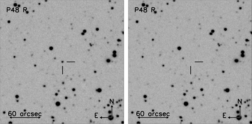
Figure 1: A combination of several Palomar 48 inch $R$-band images around the time of peak brightness of iPTF 13ajg (at left) and from before the explosion (at right); the latter image has an approximate limiting magnitude of $R=23.2$.

iPTF 13ajg was imaged with the Palomar 48 inch (P48) Oschin iPTF survey telescope equipped with a 12k $\times$ 8k CCD mosaic camera (Rahmer et al., 2008) in the Mould $R$ filter, the Palomar 60 inch and CCD camera (Cenko et al., 2006) in Johnson $B$ and SDSS $gri$, the 2.56-m Nordic Optical Telescope (on La Palma, Canary Islands) with the Andalucia Faint Object Spectrograph and Camera (ALFOSC) in SDSS $ugriz$, the 4.3-m Discovery Channel Telescope (at Lowell Observatory, Arizona) with the Large Monolithic Imager (LMI) in SDSS $r$, and with the Low Resolution Imaging Spectrograph (LRIS; Oke et al., 1995) and the Multi-Object Spectrometer for Infrared Exploration (MOSFIRE; McLean et al., 2012), both mounted on the 10-m Keck-I telescope (on Mauna Kea, Hawaii), in $g$ and $R_{s}$ with LRIS and $J$ and $K_{s}$ with MOSFIRE. All images were reduced in a standard fashion; for the P48 images this was done using the IPAC pipeline (Laher et al., 2014). The P48 observed the iPTF 13ajg field multiple times per night; to increase the depth of the P48 data, we combined all images with seeing better than 3″ over 3-day intervals before extracting the magnitude. The log of the imaging observations, where we list the 3-day averages for the P48 data, is presented in Table A.1 in the Appendix.

Aperture photometry of iPTF 13ajg was performed relative to two dozen reference stars in the field with SDSS (Fukugita et al., 1996; Ofek et al., 2012) and 2MASS (Skrutskie et al., 2006) photometry. We constructed the spectral energy distribution of the reference stars in the field from SDSS or 2MASS photometry, and derived their magnitudes in the relevant filter by using the filter transmission curve; this significantly reduces the scatter in the relative photometry in case the filter is very different from that of the SDSS or 2MASS filters, such as the P48 $R$ band. No attempt was made to subtract a reference image before measuring the SN magnitude as the host turned out to be very faint: $g_{\rm AB}\approx 27.0$ and $R_{s,\rm AB}\geq 26.0$ mag (Sect. 8). The AB magnitudes listed in Table A.1 are in the natural system of the different filters, which are very similar to the SDSS/2MASS filter set for all except the P48 $R$, P60 $B$, and Keck/LRIS $R_{s}$. The magnitude uncertainty is a combination of the measurement error and the uncertainty in the calibration derived from the scatter in the offsets with respect to the different reference stars.

Starting on 2013 April 8, long-slit low-resolution spectra of iPTF 13ajg were obtained at several different epochs with the DEep Imaging Multi-Object Spectrograph (DEIMOS; Faber et al., 2003) mounted on the 10-m Keck-II telescope, with LRIS (Oke et al., 1995) at Keck-I, and with the Dual Imaging Spectrograph (DIS) mounted on the 3.5-m Astrophysical Research Consortium (ARC) telescope at Apache Point Observatory (APO) in New Mexico. These spectra, all taken with the slit aligned with the parallactic angle (see Filippenko, 1982), were reduced, extracted, telluric corrected, and flux calibrated in a standard manner with IRAF and custom IDL routines. Cosmic rays were rejected using the recipe and routine of van Dokkum (2001). The flux calibration was performed using a standard star that was observed during the same night in the same setting and slit width as the object, and with the slit aligned with the parallactic angle. If more than one standard was observed during the night, we used the one with seeing conditions nearest to those during the iPTF 13ajg observations, thereby minimizing the slit-loss uncertainty. We note that an atmospheric dispersion corrector was used when observing with LRIS, including the last epoch spectrum which was taken at high airmass.

Table 1: Log of Spectroscopic Observations of iPTF 13ajg

Date	Telescope	Instrument	Exp. Time	Grating/Grism/Filter	Slit Width	$\lambda$ Coverage	Resolution	Seeing	Airmass
(UTC 2013)			(min.)		″	(Å)	km s-1(Å)	″
Apr. 8	Keck 2	DEIMOS	15	600ZD/GG455	0.7	4410–9640	150 (2.7)	0.9	1.05
Apr. 9	Keck 1	LRIS	20	400/3400, 400/8500	0.7	3000–10,300	230 (4.3)	0.9	1.05
Apr. 17	VLT Kueyen	X-shooter	$4\times 20$		1.0/0.9/0.9	3000–24,800	55/34/59	0.8	2.13
May 8	VLT Kueyen	X-shooter	$4\times 20$		1.0/0.9/0.9	3000–21,020	55/34/59	0.7	2.13
May 10	Keck 1	LRIS	10	600/4000, 400/8500	1.0	3130–10,260	190 (3.5)	0.9	1.09
May 18	ARC	DIS	15	B400/R300	1.5	3350–5450	250 (3.6)	1.5	1.07
June 6	Keck 2	DEIMOS	$2\times 15$	600ZD/GG455	0.8	4410–9640	160 (3.0)	0.9	1.05
June 10	Keck 2	DEIMOS	$2\times 10$	600ZD/GG455	1.0	4410–9630	180 (3.4)	0.7	1.22
July 12	Keck 2	DEIMOS	20	600ZD/GG455	0.8	4900–10,140	150 (2.7)	0.8	1.06
Sep. 9	Keck 1	LRIS	$2\times 20$	400/3400, 400/8500	0.7	5600–10,230	240 (4.5)	0.8	2.10

At two epochs close to the maximum $R$-band brightness ($R_{\rm AB}=20.28$ mag), iPTF 13ajg was also observed with the X-shooter echelle spectrograph (Vernet et al., 2011) mounted on the Kueyen 8.2-m unit of the Very Large Telescope (VLT) of the European Southern Observatory (ESO). These observations were performed in Director’s Discretionary Time (DDT; ESO program ID: 291.D-5009) by staff astronomers at Paranal in Chile. The echelle spectra of the object, flux standards, and telluric standards were reduced to bias-subtracted, flat-fielded, rectified, order-combined, and wavelength-calibrated two-dimensional spectra for all three arms (UVB, VIS, and NIR) using the Reflex package and version 2.2.0 of the X-shooter pipeline (Modigliani et al., 2010). Subsequently, the object spectra were optimally extracted, telluric corrected, and flux calibrated using custom IDL routines. The flux standard was observed with a slit much wider slit (5″) than the object spectra (1″, 0.9″, and 0.9″ for the UVB, VIS, and NIR arms, respectively). We estimated the slit loss by fitting a one-dimensional Gaussian function to the object profile along the spatial direction every 300 pixels, or 6 Å, along the dispersion axis. For each fit, we first sum 300 columns (assuming the spatial direction is along the image column) to boost the object’s signal to obtain a reliable Gaussian fit. The resulting best-fit values of the full width at half-maximum intensity (FWHM) as a function of wavelength were approximated with a low-order polynomial, and in comparison with the slit width the slit loss (again as a function of wavelength) was estimated, for which the spectra were corrected. The maximum slit losses in the UVB and VIS arms were 20% on April 17 and 13% on May 8.

Following the relative-flux calibration, all spectra were put on an absolute flux scale by tying them to the $R$-band photometry; how this was done is explained in more detail in Sect. 4. The wavelengths of all spectra were converted to vacuum and were heliocentric corrected. The log of the spectroscopic observations is shown in Table 1.

3 Photometric evolution

Figure 2 shows the resulting light curves of iPTF 13ajg. The AB magnitudes shown have been corrected for the Galactic extinction along this sightline ($E_{B-V}=0.012$ mag; Schlafly & Finkbeiner, 2011). The time axis shows the number of days in the observer’s frame (rest-frame days are given at the top) relative to the peak time of the $R$-band light curve. The latter has been determined to be 2013 April 23.6 (JD = 2456406.1) from a low-order polynomial fit to the P48 and Keck $R$-band data; this fit is shown by the solid black line in Figure 2. The corresponding peak brightness is $R_{\rm AB}=20.28$ mag.

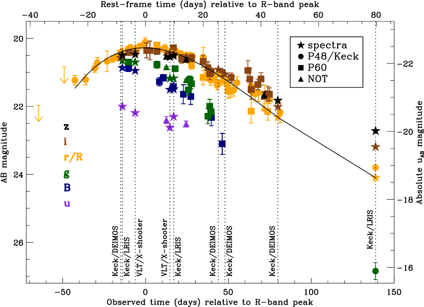
Figure 2: Light curves ($uBgRiz$) of iPTF 13ajg; the time in the observer’s (rest) frame at the bottom (top) is relative to the maximum brightness in the $R$ band. Filled circles, squares, and triangles are measurements from images obtained with the P48/Keck, P60, and NOT, respectively. For clarity, only a few prediscovery upper limits, determined using 3-day combined P48 data, are shown; see Table 1 for all relevant magnitude limits. The stars denote magnitudes derived from the flux-calibrated spectra after scaling them to the $R$-band light curve. The times at which the spectra were obtained (see Table 1) are marked with the vertical dotted lines. The right-hand axis shows the approximate absolute $u_{\rm AB}$ magnitude (corresponding to the $R$-band data), which includes a $K$ correction using the X-shooter spectrum taken on 2013 April 17. A polynomial fit to the P48+Keck $R$-band data, depicted by the solid black line, indicates that a maximum absolute magnitude of $u_{\rm AB}=-22.5$ was reached on 2013 April 23.6.

Following Hogg et al. (2002), we determine the $K$ correction from observed $R_{\rm AB}$ to rest-frame SDSS $u_{\rm AB}$ to be $K_{uR}=-0.57$ using the X-shooter spectrum from 2013 April 17. We note that since the observed $R$ band corresponds very well to rest-frame $u$ at $z=0.7403$, this $K_{uR}$ correction for iPTF 13ajg is very similar to $-2.5$ log $(1+z)$. As the iPTF 13ajg spectrum evolves with time, this $K$ correction changes from $-0.55$ for the spectra taken at tens of days before peak, to $-0.8$ for the spectra taken a month or two after peak.

Adopting a distances modulus at the iPTF 13ajg redshift ($z=0.7403$) of $\mu=43.32$ mag and a $K$ correction of $K_{uR}=-0.57$, we derive an absolute $u_{\rm AB}$-band peak magnitude of $M_{u,{\rm AB}}=-22.5$. Transforming the observed $R_{\rm AB}$ magnitude to the rest-frame Johnson $U$ and $B$ filters in the Vega system using the same spectrum results in $M_{U,{\rm Vega}}=-23.5$ and $M_{B,{\rm Vega}}=-22.2$ mag. These absolute magnitudes, which have an estimated uncertainty of 0.1–0.2 mag, are similar to those of the brightest Type I and II SNSNe to date, such as SCP 06F06 ($M_{u,{\rm AB}}=-22.2$ mag, $z=1.189$; Barbary et al., 2009), PTF 09cnd ($M_{u,{\rm AB}}=-22.1$ mag, $z=0.258$; Quimby et al., 2011), SNLS 06D4eu ($M_{U,{\rm Vega}}=-22.7$ mag, $z=1.588$; Howell et al., 2013), and CSS121015:004244+132827 ($M_{B,{\rm Vega}}=-22.6$ mag, $z=0.287$; Benetti et al., 2013). On the right-hand axis of Fig. 2 we indicate the approximate absolute magnitude $M_{\rm u}$ corresponding to the $R$-band light curve of iPTF 13ajg. Although this is correct for the values around peak, owing to the evolving $K$ correction this is only an approximation at later times.

The date of explosion of iPTF 13ajg was estimated by fitting a parabolic and exponential function to the pre-peak light curve, following Ofek et al. (2014). These two methods provide very similar dates of explosion: March 2/3 (JD = 2456354/5), which is 51/52 days (observed) before the $R$-band peak magnitude. In the rest frame, this corresponds to an exponential rise time of about a month, which is much longer than the rise times of standard core-collapse SNe of type II (Anderson et al., 2014; Sanders et al., 2014) and type Ib/c (Taddia et al., 2014). We caution that despite these two methods leading to similar date estimates, the date of explosion is highly uncertain. Moreover, the early-time (unobserved) light curve of iPTF 13ajg may have contained a plateau as was observed for SLSN 2006oz (Leloudas et al., 2012), in which case the rise time of about 30 rest-frame days should be considered a lower limit.

4 Spectral evolution

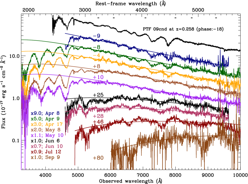
Figure 3: Time series of Keck/DEIMOS, Keck/LRIS, and VLT/X-shooter spectra of iPTF 13ajg (see Table 1). The spectra were corrected for Galactic extinction (Schlafly & Finkbeiner, 2011) and scaled to the polynomial fit to the $R$-band photometry depicted in Fig. 2. To avoid the spectra overlapping each other, an additional arbitrary scaling was applied as indicated at the bottom left, along with the civil date of observation (UTC 2013); the phase (rest-frame days relative to the $R$-band maximum) is shown next to each spectrum. The iPTF 13ajg spectra were smoothed with a Gaussian filter having a FWHM of 5 Å. The spectra were fit with a Planck function to selected 50 Å-wide wavelength regions (the same for all spectra; these regions are indicated with dashes at the top of the plot) free from apparent features, where the region blueward of rest-frame 3200 Å has been discarded owing to the presence of very strong absorption. These blackbody fits are shown by the solid lines (see also Fig. 5). For comparison, we include the Keck/LRIS spectrum of PTF 09cnd (shifted in wavelength to match that of iPTF 13ajg) at its actual flux scale (Quimby et al., 2011).

We took particular care with the relative flux calibration of the spectra (Sect. 2) and placed them on an absolute flux scale as follows. We multiplied the P48 $R$-band filter transmission curve by each spectrum and integrated the resulting flux over wavelength, did the same for the hypothetical AB standard star (which emits 3631 Jy independent of wavelength), and scaled the resulting AB magnitude to the value derived from the polynomial fit to the $R$-band light curve at that epoch. Once on this absolute scale, we derived synthetic $uBgriz$ magnitudes from each spectrum, provided that the spectrum covered (most of) the wavelength range of the corresponding transmission filter. These spectral magnitudes are shown as stars in Figure 2. The agreement between these synthetic magnitudes and the magnitudes derived from the images is fairly good (with a scatter less than 0.2 mag), even for the X-shooter spectra which were taken at high airmass, showing that the absolute and relative flux calibration of the spectra is reasonably reliable.

Figure 3 shows the time series of spectra of iPTF 13ajg, starting at $9$ rest-frame days before the $R$-band peak and ending at a phase of $+80$ days. For clarity, some of the spectra have been offset from their true absolute flux scale. At the top, we also include the spectrum of PTF 09cnd (shifted in wavelength to match that of iPTF 13ajg), a prototypical hydrogen-poor SLSN at $z=0.258$ (Quimby et al., 2011). The resemblance between iPTF 13ajg and PTF 09cnd (both lacking hydrogen features) combined with the peak absolute magnitude leads to the classification of iPTF 13ajg as a SLSN-I. The redshift, as measured from the narrow Mg I, Mg II, and Fe II absorption lines discussed in detail in Sect. 6, is 0.7403.

The spectra show very prominent broad absorption features in the rest-frame near-UV range, as well as weaker features in the rest-frame optical. The latter can be identified with blueshifted O II (the five features between $\lambda_{\rm rest}=3600$ and 4500 Å) at early times (Quimby et al., 2011). At later times broad Ca II ($\lambda_{\rm rest}\approx 3700$ Å) and probably Fe II ($\lambda_{\rm rest}\approx 3700,4300,5000$ Å) are present; that is, the spectrum of iPTF 13ajg is evolving to appear similar to spectra of SNe Ic (see Pastorello et al., 2010; Quimby et al., 2011). The identification of the near-UV features is not so unambiguous: Quimby et al. (2011) suggested that the lines at rest-frame wavelengths of 2200 Å, 2400 Å, and 2650 Å are produced by C II, Si III, and Mg II (respectively), while Howell et al. (2013) instead suggest them to be due to C III+C II, C II, and Mg II+C II. The latter authors were also able to detect a feature at 1900 Å in the spectrum of SNLS 06D4eu, which they attribute to Fe III, and it was also suggested to be present in SLSN 2006oz (Leloudas et al., 2012).

To view these features in more detail, we zoom in on the near-UV part of the relevant spectra in Fig 4. These spectra have been normalized by an approximation of the continuum obtained from fitting a Planck function to selected 50 Å-wide wavelength regions (the same for all spectra) free from apparent features. The region blueward of 5600 Å (rest-frame 3200 Å) has been discarded in the fit owing to the presence of very strong absorption. These Planck fits are shown by the solid lines in Figure 3.

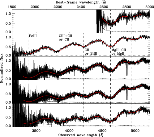
Figure 4: The blue side of the spectra taken at epochs 1–5 or phase $-9,-8,-4,+8$, and $+10$ days (top to bottom panels), normalized by the blackbody fits (see Fig. 3), are shown by the black solid lines. The spectra have not been smoothed. The corresponding error spectra are indicated with the dotted lines. Gaussian fits are shown by the solid red lines. To illustrate the evolution of the central wavelength of the lines with time, their best-fit wavelengths in the earliest epoch are marked with the vertical dashed lines. The strengths of these features evolve little to moderately over the course of 20 rest-frame days. The epoch 3 and 4 X-shooter spectra clearly display the narrow absorption features of Mg II and Fe II between 4000 Å and 5000 Å (observed); these are less significant at the other epochs owing to the lower spectral resolution. In the second panel from the top we list the line identification of the broad features according to Howell et al. (2013) (top label) and Quimby et al. (2011) (bottom label).

To derive basic quantities such as line center and strength, we fit simple Gaussian profiles to all the obvious lines present in the near-UV range. Keeping in mind the fact that the extrapolation of the continuum fits to this wavelength range is fairly uncertain, it is still interesting to note that the strength of the absorption features does not seem to vary much with time. The only exception is the feature at rest-frame 2650 Å, whose strength seems to increase at later times. The line center is independent of the continuum extrapolation. For the features at 2200 Å and 2400 Å, it evolves roughly 3000 km s^-1 to the red over the course of 20 rest-frame days. By contrast, the line center is constant for the absorption at 1900 Å (uncertain due to the low signal-to-noise ratio [S/N] at these wavelengths), 2650 Å, and 2850 Å.

Recently, an expansion velocity of $\sim$ 16,500 km s^-1 was estimated from the velocity difference between the narrow Mg II lines and the broad absorption feature for the SLSN PS1-11ap at $z=0.524$ (McCrum et al., 2014b). This is similar to those found for other SLSNe: velocities range from 10,000–20,000 km s^-1 (e.g., Quimby et al., 2011; Chomiuk et al., 2011; Inserra et al., 2013). Assuming the feature at rest-frame 2650 Å is Mg II $\lambda$2800, the expansion velocity for iPTF 13ajg is 15,500 km s^-1. In Sect. 5, we present an estimate of the blackbody radius evolution of iPTF 13ajg as a function of time, which appears to be well described by a linear increase in time until at least 50 rest-frame days after peak. The expansion velocity corresponding to this radius evolution is 11,500 km s^-1.

5 Bolometric luminosity evolution

As already mentioned in the previous section, the solid lines in Figure 3 depict blackbody fits to selected 50 Å-wide wavelength spectral regions (the same for all spectra) redward of 5600 Å (to avoid the strong absorption features in the blue) and free from apparent features. These blackbody fits result in an estimate of the temperature and radius of an expanding photosphere at each of the nine spectral epochs; these are shown by the solid circles in the top (temperature) and middle (radius) panels of Figure 5. For comparison, the open squares show the temperatures and radii as derived for the SLSN CSS121015:004244+132827 at $z=0.287$ by Benetti et al. (2013); these data points are not used in any of the fits described below.

Figure 5: Time evolution of the blackbody temperature (top panel), blackbody radius (middle), and bolometric luminosity (bottom panel) of iPTF 13ajg. The blackbody fits to the observed spectra (shown by the solid lines in Fig. 3) provide nine temperature and radius estimates, depicted with the filled circles. The down-pointing triangles in the bottom panel indicate the bolometric luminosity ($L_{\rm bol}=4\pi R^{2}\sigma T^{4}$) corresponding to these estimates. The upward-pointing triangles show the luminosities inferred from simply integrating the observed spectra over wavelength and converting the integrated flux to luminosity. The functions fit to the temperature (power law) and radius (first-order polynomial) evolution combine to produce an estimate of the bolometric luminosity evolution of iPTF 13ajg, shown by the solid line in the bottom panel. The open circles in the middle panel are the blackbody radii inferred from the P48/Keck $R$-band photometry and assuming the power-law temperature evolution; these points are included in the polynomial fit to the radius evolution. The open squares indicate the $T$ and $R$ evolution reported for the SLSN CSS121015 (Benetti et al., 2013); these points are not used in the fits. The dashed line in the bottom panel, our best estimate for the bolometric light curve, is a combination of interpolation between the available spectra, and extrapolation using the blackbody fits, which are modified in the near-UV by the Gaussian fits to the broad absorption features (see Fig. 4). Finally, the dotted line in the bottom panel indicates the light curve produced by a magnetar model with a magnetic field of $B=2.3\times 10^{14}$ G and an initial spin period of $P=1.1$ ms.

The temperature evolution of iPTF 13ajg is poorly described by a linear decline in time; instead a second-order polynomial and a power-law function ($T\propto(t-t_{0})^{\alpha}$) provide a good fit. We adopt the power-law function, as the polynomial fit results in an unphysical upturn at late times which is avoided in the power-law fit. The best-fit values for the power-law fit parameters are highly dependent on the choice of the start time $t_{0}$. For example, when fixing $t_{0}$ to $-30$ rest-frame days, $\alpha=-0.1$, with a very steep decay at early times, whereas $\alpha=-3.5$ when $t_{0}$ is unconstrained. The latter fit is shown by the solid line in the top panel of Figure 5. The photospheric radius evolution is well described by a linear increase in time, with a slope of $1.0\times 10^{14}$ cm per rest-frame day, or 11,500 km s^-1. Adopting the temperature evolution inferred above, the radius evolution can also be constrained from the imaging measurements by converting the magnitudes to flux at the effective wavelength of the corresponding filter. In the fit to the radius evolution, we have also included the P48/Keck $R$-band light-curve data, which are shown by the open circles in the middle panel of Fig. 5. We note that at phase +80, it is not clear whether the photometry or spectroscopy provides a more reliable estimate of the radius; it may well be that the radius evolution is flattening off around this phase.

These fits to the photospheric temperature and radius evolution are combined to estimate the total bolometric luminosity of iPTF 13ajg, using $L_{\rm bol}=4\pi R^{2}\sigma T^{4}$, illustrated by the solid line in the bottom panel of Figure 5. The downward-pointing triangles in this panel show the bolometric luminosity corresponding to the temperatures and radii inferred from the nine spectra. A strict lower limit can be obtained by simply integrating the observed spectra over their observed wavelength ranges, and converting the integrated flux to luminosity in the rest frame. Those values are indicated by the upward-pointing triangles in the bottom panel.

Finally, we provide a “best” estimate of the bolometric light curve of iPTF 13ajg by constructing a flux surface as a function of time and wavelength as follows. Whenever the flux at a particular wavelength at a particular time can be recovered by interpolation between the observed spectra, we do so. Before interpolation, the spectra are first median filtered to avoid introducing extreme features based on a single low or high value in one of the spectra. Each interpolated spectrum is scaled to the value of the polynomial fit to the P48/Keck $R$-band photometry (shown by the solid line in Figure 2). For wavelengths and time intervals falling outside the surface covered by the observed spectra, we adopt the blackbody model flux described by the temperature evolution power law, again combined with the P48/Keck $R$-band flux evolution. In the UV part, this flux surface is modified by the near-UV absorption features as described by the Gaussian fits discussed in the previous section. We simply extrapolate these fits to earlier and later times, assuming their strength at early times is the same as in the spectrum at epoch 2, and the same as in the epoch 5 spectrum for late times. This flux surface ranges in time from $-24$ to $+80$ days, and in wavelength from 1900 to 12,000 Å, both in the rest frame; beyond these boundaries it is assumed to be zero. The integral of this flux surface over wavelength results in the dashed line in the bottom panel of Figure 5. As the luminosity absorbed by the UV features is expected to be re-emitted at longer wavelengths, our “best” bolometric luminosity estimate (which has been corrected downward owing to the strong absorption in the UV) does not necessarily describe the true bolometric luminosity evolution of iPTF 13ajg. We expect the latter to be bracketed by the blackbody and the “best” luminosity curves, depicted by the solid and dashed lines in the bottom panel of Figure 5, respectively.

The observed bolometric peak luminosity of iPTF 13ajg is $3.2\times 10^{44}$ erg s^-1 ($6.3\times 10^{44}$ erg s^-1) assuming the “best” (blackbody) bolometric light curve. Integrating these two light curves over the time interval $-24$ to $+80$ rest-frame days leads to the following estimates of the total radiated energy of iPTF 13ajg: $1.3\times 10^{51}$ erg (“best”) and $2.5\times 10^{51}$ erg (blackbody). These values are similar to those found for other SLSNe, such as the Type I SNLS 06D4eu (Howell et al., 2013) and the Type II CSS121015:004244+132827 (Benetti et al., 2013).

Closely following Inserra et al. (2013), using their equations D1 through D7, we generated light curves using a magnetar model based on the Arnett (1982) formalism. We found that a magnetar with $B=2.27\times 10^{14}$ G, $P=1.14$ ms, $\tau_{m}=34.59$ days, and $t_{i}=-32.06$ days is consistent with our estimated range for the bolometric light curve of iPTF 13ajg, as shown by the dotted line in the bottom panel of Figure 5.

6 Narrow absorption features

The combination of X-shooter’s sensitivity and intermediate resolving power, and the brightness and significant redshift of iPTF 13ajg, resulted in the clear detection of several narrow rest-frame near-UV absorption lines. No significant variation of the absorption-line strength is detected when comparing the spectra taken on April 17 and May 8. Spectral regions around the relevant absorption lines detected in the combined spectrum are presented in Figure 6. The continuum has been normalized to unity, and a redshift of 0.7403 has been adopted as the systematic redshift of the host galaxy of iPTF 13ajg. In Table 2 we report the observed transitions, wavelengths, and rest-frame equivalent widths ($W_{r}$), plus some limits for other nondetected significant transitions. These include excited lines associated with iron and nickel, regularly detected in GRB afterglow spectra (e.g., Chen et al., 2005; Vreeswijk et al., 2007).

Table 2: Absorption-Line Parameters

Ion	$\lambda_{\rm obs}$	$W_{\rm r}$	COG			Voigt
	(Å)	(Å)	$\log N_{\rm X}$ [cm-2]	$b$ (km s-1)		$\log N_{\rm X}$ [cm-2]	$b$ (km s-1)
Fe ii $\lambda 2600$	4525.08	$0.293\pm 0.029$	$14.04^{+0.13}_{-0.07}$	$12.64\pm 0.91$		$14.25\pm 0.10$	$11.9\pm 1.1$
Fe ii $\lambda 2586$	4501.54	$0.226\pm 0.025$	. . .	. . .		. . .	. . .
Fe ii $\lambda 2382$	4146.72	$0.354\pm 0.027$	. . .	. . .		. . .	. . .
Fe ii $\lambda 2374$	4132.27	$0.134\pm 0.027$	. . .	. . .		. . .	. . .
Fe ii $\lambda 2344$	4079.63	$0.261\pm 0.030$	. . .	. . .		. . .	. . .
Mg ii $\lambda 2796$	4866.44	$0.510\pm 0.015$	$14.44^{+0.25}_{-0.20}$	(12.64)		$14.68^{+0.34}_{-0.28}$	(11.9)
Mg ii $\lambda 2803$	4878.93	$0.451\pm 0.014$	. . .	. . .		. . .	. . .
Mg i $\lambda 2852$	4965.26	$0.076\pm 0.014$	$11.82\pm 0.09$	(12.64)		$11.94\pm 0.06$	(11.9)
Mn ii $\lambda 2594$	4516.94	$<0.082$	. . .	. . .		$<12.80$	(11.9)
Mn ii $\lambda 2576$	4484.53	$<0.070$	$<12.2$	(12.64)		. . .	. . .
Mn ii $\lambda 2606$	4536.02	$<0.092$	. . .	. . .		. . .	. . .
Fe ii${}^{*}\lambda 2612$	4546.80	$<0.101$	. . .	. . .		. . .	. . .
Fe ii${}^{*}\lambda 2396$	4170.38	$<0.095$	$<12.4$	(12.64)		. . .	. . .
Fe ii${}^{*}\lambda 2626$	4570.81	$<0.090$	. . .	. . .		$<12.8$	(11.9)
Fe ii${}^{*}\lambda 2389$	4158.20	$<0.083$	. . .	. . .		. . .	. . .
Fe ii${}^{*}\lambda 2365$	4116.77	$<0.077$	. . .	. . .		. . .	. . .
Fe ii${}^{*}\lambda 2333$	4061.02	$<0.111$	. . .	. . .		. . .	. . .
Fe ii${}^{5*}\lambda 2360$	4108.36	$<0.078$	$<13.54$	(12.64)		$<14.0$	(11.9)
Fe ii${}^{5*}\lambda 2348$	4087.68	$<0.094$	$<13.42$	(12.64)		$<13.9$	(11.9)
Fe ii${}^{5*}\lambda 2332$	4058.42	$<0.107$	. . .	. . .		. . .	. . .
Ni ii${}^{**}\lambda 2316$	4031.84	$<0.120$	$<13.06$	(12.64)		$<13.4$	(11.9)
Ni ii${}^{**}\lambda 2217$	3858.54	$<0.234$	$<13.18$	(12.64)		. . .	. . .

We performed Voigt profile fitting of the absorption lines to infer the column densities. For completeness, we explored the lines’ parameters by using two other different methods: the apparent optical depth (AOD; Savage & Sembach, 1991) and the curve of growth (COG; Spitzer, 1978). Although we are not in the ideal situation of high spectral resolution ($R\mathrel{\hbox{\hbox to0.0pt{\lower 2.36806pt\hbox{$\sim$}\hss}\kern 0.0pt\raise 1.72218pt\hbox{$>$}}}40,000$) and signal-to-noise ratio ($S/N>30$), comparing results from these different tools allows us to evaluate the reliability of the resulting column densities. These are summarized in Table 2 for the COG and Voigt profiles; the AOD results do not provide additional information so they are not included in the table. Adopting the Voigt profile values, we find log $N$(Mg I) $=11.94\pm 0.06$, log $N$(Mg II) $=14.7\pm 0.3$, and log $N$(Fe II) $=14.25\pm 0.10$. The relative magnesium over iron abundance is [Mg/Fe] $=0.3\pm 0.3$. In principle, this quantity can be used to infer the amount of dust in a similar way as is done for [Zn/Fe] (see De Cia et al., 2013); however, the large uncertainty in the observed [Mg/Fe] prevents us from drawing any conclusions about the dust depletion.

The absorption lines are in one single and narrow component. Being narrow is an indication that the absorbing gas is not associated with the supernova ejecta, for which features are generally very broad and blueshifted with respect to the rest-frame velocity (see, e.g., Fig. 3). In Sect. 7 we derive a lower limit on the distance between the iPTF 13ajg and the absorbing gas responsible for the narrow lines, showing that these lines are produced by gas in the interstellar medium (ISM) of the host galaxy of iPTF 13ajg.

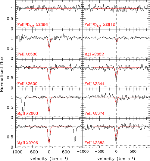
Figure 6: Spectral regions centered on absorption lines of Mg I, Mg II, and Fe II, associated with neutral gas, in the averaged X-shooter spectrum (black solid line). No other narrow absorption lines are detected. The spectrum has been normalized to unity by fitting a low-order polynomial to the surrounding continuum. The red solid line indicates the best-fitting Voigt profile, from which we infer the column densities (Table 2). In the top panels, we also show the expected location of the strongest transitions of the first excited level of Fe II, ⁶D_7/2, which are not detected.

We determined a small effective Doppler width, $b\approx 12$ km s^-1, in a single component, indicating that the low-ionization gas is distributed in a region with a small velocity dispersion along the sight line. The low ionization state is indicated by the presence of Mg I, Mg II, and Fe II. Owing to the limited resolution and resolving power, we cannot exclude that the intrinsic absorption is originating in more than one cloud.

However, we still can limit these clouds to be distributed over a velocity range smaller than $\sim 100$ km s^-1. Following Ledoux et al. (2006) (see also Møller et al., 2013), we measure the line profile velocity width, $\Delta V$, defined by the wavelengths where the cumulative apparent optical depth profile is equal to 5% and 95%: $\Delta V=c[\lambda(95\%)-\lambda(5\%)]/\lambda_{0}$ km s^-1, where $c$ is the speed of light. We use the absorption lines Fe II $\lambda$$\lambda$2374,2586,2600 and Mg II $\lambda$2803 and find $\Delta V\approx 76$ km s^-1. This value is only moderately higher than the resolving power in the UVB arm of X-shooter (55 km s^-1), which implies that the true $\Delta V$ of iPTF 13ajg could be lower. Moreover, the absorption lines used may be somewhat saturated, which would also lead to an overestimate of the intrinsic $\Delta V$ value. Compared to the QSO damped Ly$\alpha$ absorber (DLA) sample of Ledoux et al. (2006), the iPTF 13ajg absorber is among the 30% lower velocity DLAs, even though the UVES resolution of the Ledoux et al. sample allows the $\Delta V$ to be constrained down to much lower velocities (20 km s^-1 or so). Using the QSO-DLA velocity-metallicity relations as shown in the left panel of Figure 4 of Ledoux et al. (2006), and considering the iPTF 13ajg $\Delta V$ that we measure as an upper limit, we can obtain a very crude limit on the metallicity along the iPTF 13ajg sightline: [M/H] $\lesssim-1$. One additional caveat in this comparison is that the low-redshift QSO-DLA sample of Ledoux et al. (2006) is at $1.7<z<2.43$, while the redshift of iPTF 13ajg is much lower, $z=0.7403$. Using the redshift evolution of the DLA mass-metallicity relation as measured by Møller et al. (2013) (see their Figure 2), we estimate [M/H] $\lesssim-0.7$ for the host galaxy of iPTF 13ajg.

7 Distance between iPTF 13ajg and Fe II gas

We estimate a lower limit on the distance between the supernova and the Fe II and Mg II material from the absence of fine-structure lines, similar to what has been done for GRB afterglows (e.g., Vreeswijk et al., 2007). The ultraviolet photons from the GRB afterglow or SLSN will excite any Fe II material that is near enough. At sufficient photon fluxes, a significant fraction of the atoms will be excited to levels just above the ground state. In the case of GRB afterglows, absorption lines from these excited levels of ions such as Si II (Vreeswijk et al., 2004; Savaglio et al., 2012), Fe II (Chen et al., 2005; Prochaska et al., 2006), and Ni II have been detected along tens of sightlines. The GRB-cloud distances inferred from these observations range from about 50 pc to well over a kiloparsec (e.g., Vreeswijk et al., 2007; D’Elia et al., 2009; Vreeswijk et al., 2013).

To our knowledge, the only SN in which such fine-structure lines have been detected to date is the Type IIn SN 1998S (Bowen et al., 2000). Their detection is challenging in the case of SNe, as spectroscopic observations at intermediate resolving power or higher in the near-UV are required. SLSNe, being very luminous and UV bright, in principle allow the detection of these fine-structure lines from the ground, as they are sufficiently bright to obtain a good S/N at the relevant optical wavelengths.

Figure 7: Expected population of the first excited level of Fe II (⁶D_7/2, indicated with the dashed lines) due to excitation by UV photons released by iPTF 13ajg, if the Fe II atoms were located at a distance of 10 pc, 50 pc, and 100 pc from the UV source. The upper limit on the column density, log $N$(Fe II ⁶D_7/2) $<$ 12.4, shows that the Fe II atoms (as detected by the narrow absorption lines) are at least 50 pc away from iPTF 13ajg.

For iPTF 13ajg, we measured a column density for Fe II of log $N$(Fe II) $=14.25\pm 0.10$, while constraining the population in the first excited level to be log $N$(Fe II ⁶D_7/2) $<$ 12.4. We calculate the excitation of the Fe II ions, closely following the method described by Vreeswijk et al. (2013), assuming different distances between iPTF 13ajg and the absorbing material. This provides the population of different excited levels, including the first excited level ⁶D_7/2, as a function of time. For the input light curve, we adopt the “best” flux evolution as a function of time and wavelength of iPTF 13ajg that was described in Sect. 5, starting at 30 rest-frame days before the $R$-band peak. We note that this does not include a potential early-time UV flash; if present, such a flash would increase the amount of excitation and would therefore increase the lower limit on the distance inferred below. Since the amount of ionizing flux at rest-frame wavelengths below 912 Å from iPTF 13ajg is not expected to be high due the large opacity of the ejected material in the UV wavelength range, even at early times (see Fig. 3), we neglect ionization in the modelling. Even in case iPTF 13ajg would be emitting a considerable amount of ionizing photons, the estimated H I column density associated with the metal absorption lines is of the order of log N(H I) $\approx$ 20 (see Sect. 9), which is sufficient to shield the absorber from most photons capable of ionizing Fe II.

The Fe II excitation is caused by UV photons with wavelengths from the Lyman limit up to about 2600 Å. We conservatively assume that the iPTF 13ajg flux is negligible for rest-frame wavelengths below 1900 Å. If there is significant flux present in that wavelength region, the inferred lower limit on the distance would increase, since the amount of excitation would be underestimated. The dashed lines in Figure 7 show the expected time evolution of the Fe II ⁶D_7/2 level, assuming a distance of 10 pc (top dashed line), 50 pc (middle), and 100 pc (bottom). For all three calculations, the ground-level population is indicated with the same solid line. The upper limit on the ⁶D_7/2 level column density constrains the distance between iPTF 13ajg and the Fe II absorption that we observe to be at least 50 pc. If the Fe II ions were much closer, we should have detected significant absorption lines from this level.

8 The host galaxy of iPTF 13ajg

We secured late-time images of the field of iPTF 13ajg with Keck/LRIS on 2013 September 9, 2014 April 28, and July 30 using filters $g$ and $R_{s}$ on all three nights. These dates correspond to 80, 213, and 267 rest-frame days after the $R$-band peak magnitude. In $g$, the magnitudes at these epochs are $26.89\pm 0.25$, $26.49\pm 0.14$, and $>26.9$, respectively (all AB; see Table 1). The bright April measurement may have been due to a rebrightening of the supernova. Although the host is formally not detected in the July measurement, it appears to be present at the 2.5$\sigma$ level. Summing the September 9 and July 30 images, we find $g=26.8\pm 0.2$ mag; this combined image is shown in Figure 8. From the Keck $R_{s}$-band images, we measure $23.83\pm 0.08$, $24.84\pm 0.09$, and $26.01\pm 0.22$ mag at 80, 213, and 267 days, respectively (all AB; see Table 1). Even in the last $R$-band epoch the SN may still be contributing to the flux. The $g$-band detection ($g_{\rm AB}\approx 27.0$ mag) and the limiting $R_{s}$-band measurement ($R_{s,\rm AB}\geq 26.0$ mag) roughly correspond to an absolute $B$-band magnitude $M_{B,{\rm Vega}}\gtrsim-17.7$ for the host of iPTF 13ajg. On 2014 February 13, or a phase of 170 days, we also imaged the field with DCT/LMI in the SDSS $r$ band. We do not detect iPTF 13ajg or its host, and derive a limiting magnitude of $r>25.12$. In addition, we imaged the field of iPTF 13ajg in the near-infrared with Keck/MOSFIRE on 2014 June 7 in $K_{s}$ and on 2014 June 8 in $J$. We do not detect any source at the location of iPTF 13ajg and derive the following limiting AB magnitudes: $J>23.5$ and $K_{s}>23.1$ (see Table 1).

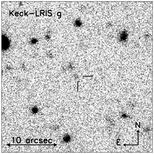
Figure 8: Keck/LRIS $g$-band image of the host galaxy of iPTF 13ajg; it is the sum of the 2013 September 9 and 2014 July 30 observations. The position of the early-time supernova, indicated at the center, has been projected onto this image using NOT images from 2013 May 5 and several stars in the field for the alignment; the uncertainty in the projection is 0.4 pixels (0.05″), too small to show. We measure the host-galaxy magnitude to be $g_{\rm AB}\approx 27.0$.

Using NOT images of iPTF 13ajg around peak magnitude, we project the position of the supernova onto the sum of the 2013 September and 2014 July Keck $g$-band images, shown by the crossbars in Figure 8. The uncertainty in this projection is 0.4 LRIS pixels (0.05″). There does not appear to be a significant offset between the location of the SN and the peak of the galaxy light. There is an additional object about 3″ to the northeast of the iPTF 13ajg location, which might be related to the host galaxy of iPTF 13ajg, but given its faintness and the relatively large offset it is more likely to be unrelated.

No emission lines are detected at the redshift of iPTF 13ajg in any of our spectra. We determined the most stringent limits on the [O II] $\lambda$3727, [O III] $\lambda$5007, and H$\alpha$ observed line fluxes to be $1.5\times 10^{-18}$ erg s^-1 cm^-2, $1.5\times 10^{-18}$ erg s^-1 cm^-2, and $4.6\times 10^{-18}$ erg s^-1 cm^-2, respectively. Adopting the apparent host-galaxy $g$-band magnitude of $g=27.0$ as the continuum flux (corresponding to $8.8\times 10^{-20}$ erg s^-1 cm^-2 Å^-1), these flux limits correspond to the following rest-frame equivalent-width limits: $W_{r}({\rm[O~{}II]~{}\lambda 3727})<10$ Å, $W_{r}({\rm[O~{}III]~{}\lambda 5007})<10$ Å, and $W_{r}({\rm H\alpha})<30$ Å.

We convert the [O II] and H$\alpha$ flux limits to star-formation rate (SFR) limits of SFR${}_{\rm[O~{}II]}<0.07~{}\mbox{M${}_{\odot}$ yr${}^{-1}$}$ and SFR${}_{\rm H\alpha}<0.15~{}\mbox{M${}_{\odot}$ yr${}^{-1}$}$, using the [O II]-SFR conversion derived by Savaglio et al. (2009) for low-luminosity star-forming GRB host galaxies at $z<0.5$ and the H$\alpha$-SFR conversion provided by Kennicutt (1998). In the [O II] flux-to-SFR conversion, we have conservatively increased the limit by a factor of 3.4, which is twice the dispersion of the [O II]-SFR conversion factor (see Savaglio et al., 2009). In the H$\alpha$ conversion we use the initial mass function (IMF) of Baldry & Glazebrook (2003); this results in an SFR that is a factor of 1.8 lower than when adopting a Salpeter IMF. We note that we have not included any dust or slit-loss corrections in these SFR limits. As an example, an extinction of $A_{V}=0.5$ mag would increase the SFR${}_{\rm[O~{}II]}$ limit by a factor of about two. From the lack of absorption at the expected wavelengths of the Na I D doublet, we can constrain the host-galaxy extinction. The upper limit on the equivalent width of Na I D2 of $W_{\rm rest}<0.5$ Å (the spectrum S/N around the expected wavelength of this line is 2.5-3) provides $E_{B-V}<0.12$ mag (Poznanski et al., 2012), or $A_{V}\lesssim 0.4$ mag. Given the very small amount of neutral metal absorption, the extinction along the iPTF 13ajg sight line and in the host galaxy is likely smaller than the limit inferred from Na I D: $A_{V}\lesssim 0.1$ mag.

We searched for potential diffuse interstellar bands (DIBs), but do not detect any. DIBs have been successfully detected in the host galaxies of SN 2001el and SN 2003hn (Sollerman et al., 2005) and have been observed to vary with time in spectra of the broad-lined Type Ic supernova SN 2012ap (Milisavljevic et al., 2014). The S/N of the X-shooter spectra in the near-infrared region, where the iPTF 13ajg DIBs would be located, is so low (S/N $\approx 3$) that we cannot put meaningful constraints on their strength.

9 Discussion

Gas clouds similar to the one in the host of iPTF 13ajg are observed in halos of high-redshift galaxies. Mg II absorbers are routinely detected in QSO spectra (e.g., Nestor et al., 2005; Kacprzak et al., 2011). QSO Mg II absorption equivalent widths at $0.07<z<1.1$ as a function of galaxy impact parameter have recently been reported by Nielsen et al. (2013). About 60% of the detections have equivalent widths above the one detected in iPTF 13ajg: $W_{r}(2796)=0.51\pm 0.02$ Å. This fraction increases to 74% when considering the absorbers within 20 kpc of their galaxy counterpart. Compared to the sample of Mg II absorbers with impact parameters to their galaxy counterparts collected by Chen et al. (2010), this latter number is very similar: 78% of absorbers within 20 kpc of a galaxy have a larger Mg II $\lambda$2796 equivalent width than the iPTF 13ajg absorber. The Mg II $\lambda$2796 equivalent width of iPTF 13ajg is lower than all but one of a sample of 23 sub-DLAs (absorbers along QSO sightlines with $19\lesssim$ log $N$(H I)${}_{\rm sub-DLA}<20.3$) at $z<1.5$ (Meiring et al., 2008; Péroux et al., 2008; Meiring et al., 2009). This shows that the gas column density along the sightline to iPTF 13ajg is low compared to a sample of random sightlines through galaxies in the foreground of QSOs. Following Ellison (2006), we calculate the $D$-index, which can help determine whether a Mg II absorber is a DLA (with log $N$(H I) $\geq 20.3$), when the H I column density is not known. For iPTF 13ajg, $D=1000\times W_{r}(2796)/\Delta V=6.7$ (with $\Delta V=76$ km s^-1; Sect. 6); this value is higher than the recommended $D$-index DLA threshold of 5.1 for our resolution, and therefore the iPTF 13ajg absorber has a reasonable probability ($\sim 90$%) of being a DLA.

Lunnan et al. (2013) have recently studied a sample of 31 host galaxies of hydrogen-poor SLSNe, showing that SLSN-I hosts appear to have some similarities to GRB hosts. We note that, although unbiased samples of GRB host galaxies do exist (e.g., Hjorth et al., 2012), the sample of GRB hosts that Lunnan et al. use to compare with SLSNe (mostly from Svensson et al., 2010) is biased toward brighter GRB hosts. For the SLSN-I sample, on the other hand, host galaxies that are not detected are included in the analysis. Also, the most massive SLSN host galaxy in the sample of Lunnan et al. (2013) is that of PS1-10afx, which was shown by Quimby et al. (2013b) to be a gravitationally lensed SN Ia.

An interesting alternative method of probing the environments of SLSNe, thereby providing a potential way to constrain the nature of the progenitor, is through absorption-line spectroscopy. In this paper we present the first Mg I, Mg II, and Fe II column-density measurements of a SLSN, thanks to the sensitivity and intermediate resolving power of X-shooter. Normally, spectra of SLSNe are observed at low resolution, which allows only for the measurement of the equivalent width of the absorption features.

Table 3: Absorption-line strengths in Type I SLSNe

ID	$z$	$W_{\rm r}$ (Å)			Ref.
		Fe II $\lambda$2600	Mg II $\lambda$2800	Mg I $\lambda$2852
SN 2005ap	0.2832	$<0.8$	$2.92\pm 0.16$	$0.39\pm 0.10$	1
SN 2006oz	0.396	$<3.0$	$3.43\pm 0.84$	$<1.2$	2
SCP 06F6	1.189	$<0.5$	$0.93\pm 0.24$	$<0.3$	6,4
PS1-10ky	0.9558	$<0.7$	$1.87\pm 0.19$	$\cdots$	3
PS1-10awh	0.9084	$<1.0$	$2.79\pm 0.32$	$<0.8$	3
PTF 09atu	0.501	$\cdots$	$2.21\pm 0.16$	$0.51\pm 0.08$	4
PTF 09cnd	0.258	$\cdots$	$2.69\pm 0.15$	$0.33\pm 0.09$	4
PTF 09cwl	0.349	$\cdots$	$1.02\pm 0.13$	$0.42\pm 0.09$	4
PTF 10cwr	0.230	$<1.0$	$3.53\pm 0.24$	$<0.45$	4
SNLS-06D4eu	1.588	$<1.2$	$2.78\pm 0.51$	$<1.3$	5
SNLS-07D2bv	1.50	$<1.5$	$4.40\pm 0.59$	$<1.8$	5
SN 2013dg	0.26	$<0.7$	$<0.4$	$<0.2$	7

Note. — References: [1] Quimby et al. (2007); [2] Leloudas et al. (2012); [3] Chomiuk et al. (2011); [4] Quimby et al. (2011); [5] Howell et al. (2013); [6] Barbary et al. (2009); [7] Nicholl et al. (2014).

Using published spectra of hydrogen-poor SLSNe available through the Weizmann interactive SN data repository (WISeREP; Yaron & Gal-Yam, 2012), we have measured $W_{\rm r}$ of the Mg I $\lambda$2852 and Mg II $\lambda\lambda$2796, 2803 absorption lines for about a dozen SLSNe-I. We also attempted to measure the same quantity for the Fe II $\lambda$2600 absorption line, but the low redshift and/or low S/N of the spectra in the blue results in the nondetection of this line in most cases. Table 3 lists the SNe with publicly available spectra for which the SN redshift is sufficiently high ($z\gtrsim 0.2$) for the relevant transitions to shift into the wavelength range covered by the spectra. We report upper limits in cases where the line is covered by the spectrum but not detected. Most spectra lack an associated error spectrum; we therefore estimate the flux error per pixel by measuring the scatter in the continuum free from absorption lines and close to the relevant transition. The normalized flux error, the number of pixels used in the equivalent width measurement, and the pixel size in Å determine the uncertainty in the equivalent width.

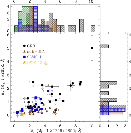
Figure 9: Comparison of the rest-frame Mg I $\lambda$2852 and Mg II $\lambda\lambda$2796, 2803 equivalent widths ($W_{\rm r}$) measured in spectra of GRB afterglows (black circles; de Ugarte Postigo et al., 2012), sub-DLAs in the foreground of background QSOs (brown triangles; Meiring et al., 2008; Péroux et al., 2008; Meiring et al., 2009), and hydrogen-poor SLSNe with published spectra (blue squares; see Table 3 for details). The average strength of the Mg I and Mg II absorption in SLSN host galaxies is significantly lower than in GRB hosts, and is similar to that of sub-DLAs. The measurements for iPTF 13ajg are indicated with the orange star. In the Mg II histogram, we also plot (in green) a sample of Mg II absorbers along QSO sightlines that are within 20 kpc of a nearby galaxy (Nielsen et al., 2013). The histograms (which do not include the upper limits) of the Mg II absorbers and sub-DLAs have been normalized to match the peak of the SLSN histograms.

In Figure 9, we compare the $W_{r}$ of Mg I and Mg II (sum of $\lambda$2796 and $\lambda$2803) of a sample of hydrogen-poor SLSNe with those measured for GRBs, taken from de Ugarte Postigo et al. (2012), and a sample of sub-DLAs in the foreground of background QSOs (Meiring et al., 2008; Péroux et al., 2008; Meiring et al., 2009). The GRB sample includes a total of 69 afterglows in the redshift range $0.12<z<6.7$ with low-resolution optical spectroscopy available. We include all GRBs (28) for which de Ugarte Postigo et al. (2012) list detections and/or upper limits for both the Mg I and Mg II host-galaxy absorption lines. The redshift range for this subsample is $0.4<z<2.4$ with a median value of $z=1.2$. The sub-DLA sample redshift range is $0.68<z<1.55$ with a median of $z=0.95$. For the SLSN-I sample, the redshift range is $0.2<z<1.6$ with a median of $z=0.5$.

On average, the absorption-line strengths in the environments of SLSNe are lower than those measured for GRB host galaxies. Applying a Kolmogorov-Smirnov (KS) test (see Press et al., 1992), we find a probability that the GRB and SLSN Mg I and Mg II distributions are taken from the same parent population to be 0.16% and 2.3%, respectively. Performing the same KS tests when compared to the sub-DLA sample, the corresponding Mg I and Mg II probabilities are 61% and 27%, respectively. This suggests that the environments of SLSNe and GRBs are different (see van den Heuvel & Portegies Zwart, 2013). We note that this inference would not be in disagreement with SLSNe and GRBs exploding in galaxies that appear to be similar, as argued by Lunnan et al. (2013).

It is important to note that even though the difference in absorption strengths in SLSN and GRB hosts appears to be significant, it might be that the sample of SLSNe is biased toward sightlines having low extinction and hence low gas column densities. GRB afterglows in principle suffer from the same bias, and they are detected at higher redshifts, leading to the observed extinction to be higher, on average, for GRB sightlines than for SLSNe. But since GRBs are also much brighter at early times, only the dustier sightlines are being missed in the GRB case. For SLSNe the bias could be significant, also because the redshift needs to be $z\gtrsim 0.2$ for the Mg absorption lines to shift into the optical range and for the SN to make it onto Figure 9; this redshift requirement results in apparently fainter SNe, which are more difficult to detect. On the other hand, several of the targets listed in Table 3 have peak magnitudes well above the limiting magnitude of the survey that discovered them, which suggests that this bias is probably not too important.

In summary, a strong bias is not likely to be present, and Figure 9 provides a strong indication that the environments of SLSNe-I and GRBs are different. In any case, expanding the number of SLSNe with measurements of the strength of narrow low-ionization ISM absorption lines, using either equivalent widths but preferably column densities, can provide useful clues to the place of birth and progenitor nature of SLSNe (see also Berger et al., 2012).

Different models have been invoked for explaining the energetics observed in hydrogen-poor SLSNe, such as a pair-instability SN (Barkat et al., 1967; Gal-Yam et al., 2009), the interaction of the SN ejecta with a dense circumstellar medium (Chevalier & Irwin, 2011; Blinnikov & Sorokina, 2010; Chatzopoulos et al., 2013), additional energy injection by a highly magnetized millisecond pulsar or magnetar (Kasen & Bildsten, 2010; Woosley, 2010), or fall-back accretion (Dexter & Kasen, 2013). The late-time decay of iPTF 13ajg is too rapid for the light curve to be powered by radioactive decay of ⁵⁶Ni, and therefore the pair-instability SN is not compatible with the observations of iPTF 13ajg. In the interaction model, the circumstellar medium is required to be hydrogen-poor given the lack of narrow hydrogen emission lines in the spectra of iPTF 13ajg; such a medium could potentially have been created by a pulsational pair-instability SN (Woosley et al., 2007; Chatzopoulos & Wheeler, 2012; Ben-Ami et al., 2014).

Interestingly, the less energetic cousins of the hydrogen-rich (Type II) superluminous SNe, the SNe IIn, are usually found in regions of their host galaxies with little recent star formation as traced by H$\alpha$ (Habergham et al., 2014). Such a location distribution would be compatible with the absorption-line strengths that we measured for a sample of H-poor SLSNe. Although the bolometric light curve of iPTF 13ajg is consistent with additional energy input from a magnetar with a magnetic field strength of $B=2.3\times 10^{14}$ G and an initial spin period of $P=1.1$ ms (Sect. 5), similar to what has been found for other hydrogen-poor SLSNe (e.g., Inserra et al., 2013), given the generic nature and flexibility of the magnetar model it would be premature to conclude that it accounts for the energetics of iPTF 13ajg. Perhaps owing to their generic nature, magnetars have also been invoked as a possible central engine of GRBs (e.g., Usov, 1992; Zhang & Mészáros, 2001; Bucciantini et al., 2009).

Placing iPTF 13ajg at higher redshifts, assuming our best estimate for the flux evolution as a function of time and wavelength (Sect. 5), it would have an apparent peak magnitude of $z_{\rm AB}=22.5$ and $24.5$ at redshifts of 2 and 3, respectively. Therefore, the next generation of 30-m class telescopes, such as the European Extremely Large Telescope (E-ELT) and the Thirty Meter Telescope (TMT), will be capable of studying in detail the host-galaxy ISM of superluminous explosions at an age of the Universe when the star-formation activity was peaking. These redshifts will also allow the detection of Ly$\alpha$ absorption from the ground, making it possible to measure H I column densities and metallicities.

10 Conclusions

We have presented an extensive imaging and spectroscopic campaign on a superluminous supernova discovered by the intermediate Palomar Transient Factory: iPTF 13ajg. This is one of the most luminous SNe to date, with an absolute magnitude at peak of $M_{u,{\rm AB}}=-22.5$ ($M_{U,{\rm Vega}}=-23.5$, $M_{B,{\rm Vega}}=-22.2$ mag).

We infer the photospheric radius and temperature evolution as a function of time using the nine epochs of Keck and VLT spectra spanning the phases from $-9$ to $+80$ days, from which we estimate the bolometric light curve. The observed bolometric peak luminosity of iPTF 13ajg is $3.2\times 10^{44}$ erg s^-1, while the estimated total radiated energy is $1.3\times 10^{51}$ erg. The bolometric light curve is consistent with a highly magnetized, rapidly rotating neutron star spinning down and providing its rotational energy to boost the supernova energetics. However, owing to the generic nature and flexibility of the magnetar model, it would be premature to conclude that it is accounting for the energetics of iPTF 13ajg.

Intermediate-resolution spectra ($R\approx 6000$) of iPTF 13ajg obtained with X-shooter enabled us to infer the metal column densities of the following UV absorption-line features: log $N$(Mg I) $=11.94\pm 0.06$, log $N$(Mg II) $=14.7\pm 0.3$, and log $N$(Fe II) $=14.25\pm 0.10$. These column densities, as well as Mg I and Mg II equivalent widths of a sample of hydrogen-poor SLSNe taken from the literature, are at the low end of those derived for GRBs, also sites of massive-star formation. This suggests that the environments in which SLSNe and GRBs explode are different. From the nondetection of Fe II fine-structure absorption lines, we derive a strict lower limit on the distance between the SN and the narrow-line absorbing gas of 50 pc. The velocity width of the features is narrow, $\Delta V=76$ km s^-1, indicating a low-mass host galaxy with an estimated metallicity of [M/H] $\lesssim-0.7$.

No host-galaxy emission lines are detected, leading to an upper limit on the star-formation rate of SFR${}_{\rm[O~{}II]}<0.07~{}\mbox{M${}_{\odot}$ yr${}^{-1}$}$. Late-time imaging shows the host galaxy of iPTF 13ajg to be faint, with $g_{\rm AB}\approx 27.0$ and $R_{\rm AB}\geq 26.0$ mag.

Table 1: Log of imaging observations of iPTF 13ajg

MJD	JD-JDRpeak	Phase	Telescope	Exp. Time	Filter	Seeing	Magnitude
(days)	(days)	(days)		(min)		″	AB
56324.553	-81.047	-46.571	P48	$2\times 1.0$	$R$	2.5	$>$ 21.43
56327.550	-78.050	-44.849	P48	1.0	$R$	2.5	$>$ 21.50
56341.043	-64.557	-37.095	P48	$2\times 1.0$	$R$	2.6	$>$ 22.00
56356.484	-49.116	-28.223	P48	1.0	$R$	2.7	$>$ 20.87
56362.969	-42.631	-24.496	P48	$6\times 1.0$	$R$	2.8	21.26 $\pm$ 0.14
56365.545	-40.055	-23.016	P48	$3\times 1.0$	$R$	2.5	21.67 $\pm$ 0.43
56367.502	-38.098	-21.892	P48	$2\times 1.0$	$R$	2.7	$>$ 20.31
56369.448	-36.152	-20.773	P48	$3\times 1.0$	$R$	2.8	21.24 $\pm$ 0.15
56372.390	-33.210	-19.083	P48	$3\times 1.0$	$R$	2.7	$>$ 19.89
56374.945	-30.655	-17.615	P48	$6\times 1.0$	$R$	2.7	20.91 $\pm$ 0.12
56376.452	-29.148	-16.749	P48	$3\times 1.0$	$R$	2.2	20.75 $\pm$ 0.15
56382.382	-23.218	-13.341	P48	1.0	$R$	2.8	20.70 $\pm$ 0.30
56385.884	-19.716	-11.329	P48	$6\times 1.0$	$R$	2.7	20.64 $\pm$ 0.10
56387.956	-17.644	-10.138	P48	$4\times 1.0$	$R$	2.9	20.58 $\pm$ 0.10
56389.389	-16.211	-9.315	P48	$3\times 1.0$	$R$	2.6	20.59 $\pm$ 0.09
56394.993	-10.607	-6.095	P48	$3\times 1.0$	$R$	2.6	20.34 $\pm$ 0.08
56396.325	-9.275	-5.330	P48	$3\times 1.0$	$R$	3.0	20.30 $\pm$ 0.09
56399.891	-5.709	-3.280	P48	$6\times 1.0$	$R$	2.9	20.44 $\pm$ 0.07
56401.899	-3.701	-2.127	P48	$6\times 1.0$	$R$	2.9	20.26 $\pm$ 0.07
56403.882	-1.718	-0.987	P48	$6\times 1.0$	$R$	2.2	20.23 $\pm$ 0.06
56405.397	-0.203	-0.117	P48	$3\times 1.0$	$R$	2.5	20.14 $\pm$ 0.13
56412.775	7.175	4.123	P48	$5\times 1.0$	$R$	2.7	20.39 $\pm$ 0.10
56415.852	10.252	5.891	P48	$6\times 1.0$	$R$	2.4	20.34 $\pm$ 0.07
56417.306	11.706	6.726	P48	$2\times 1.0$	$R$	3.1	20.32 $\pm$ 0.10
56422.881	17.281	9.930	P48	$6\times 1.0$	$R$	2.5	20.42 $\pm$ 0.06
56424.839	19.239	11.055	P48	$6\times 1.0$	$R$	2.5	20.46 $\pm$ 0.06
56426.743	21.143	12.149	P48	$5\times 1.0$	$R$	2.7	20.47 $\pm$ 0.07
56428.571	22.971	13.199	P48	$4\times 1.0$	$R$	2.7	20.57 $\pm$ 0.11
56431.886	26.286	15.104	P48	$6\times 1.0$	$R$	2.5	20.68 $\pm$ 0.09
56433.845	28.245	16.230	P48	$6\times 1.0$	$R$	2.5	20.56 $\pm$ 0.10
56440.358	34.758	19.972	P48	$2\times 1.0$	$R$	3.0	20.58 $\pm$ 0.29
56442.902	37.302	21.434	P48	$4\times 1.0$	$R$	2.5	21.13 $\pm$ 0.15
56444.810	39.210	22.531	P48	$4\times 1.0$	$R$	2.3	21.26 $\pm$ 0.14
56446.752	41.152	23.646	P48	$4\times 1.0$	$R$	2.1	21.22 $\pm$ 0.12
56448.747	43.147	24.793	P48	$4\times 1.0$	$R$	2.2	21.41 $\pm$ 0.14
56450.748	45.148	25.943	P48	$4\times 1.0$	$R$	2.3	21.04 $\pm$ 0.11
56452.744	47.144	27.090	P48	$4\times 1.0$	$R$	2.5	21.27 $\pm$ 0.13
56454.739	49.139	28.236	P48	$4\times 1.0$	$R$	2.3	21.39 $\pm$ 0.15
56456.738	51.138	29.385	P48	$4\times 1.0$	$R$	2.3	21.60 $\pm$ 0.18
56458.735	53.135	30.532	P48	$4\times 1.0$	$R$	2.2	21.55 $\pm$ 0.18
56460.730	55.130	31.678	P48	$4\times 1.0$	$R$	2.3	21.33 $\pm$ 0.18
56462.727	57.127	32.826	P48	$4\times 1.0$	$R$	2.4	$>$ 21.93
56469.205	63.605	36.548	P48	$2\times 1.0$	$R$	2.1	21.43 $\pm$ 0.23
56471.718	66.118	37.992	P48	$4\times 1.0$	$R$	2.4	21.66 $\pm$ 0.21
56473.718	68.118	39.142	P48	$4\times 1.0$	$R$	2.2	21.62 $\pm$ 0.26
56475.805	70.205	40.341	P48	$4\times 1.0$	$R$	2.6	$>$ 21.68
56477.297	71.697	41.198	P48	$2\times 1.0$	$R$	2.2	21.68 $\pm$ 0.28
56486.725	81.125	46.616	P48	$4\times 1.0$	$R$	2.1	22.21 $\pm$ 0.30
56488.800	83.200	47.808	P48	$4\times 1.0$	$R$	2.3	$>$ 22.26
56490.904	85.304	49.017	P48	$3\times 1.0$	$R$	2.7	$>$ 20.97
56395.324	-10.276	-5.905	P60	2.0	$i$	1.6	20.44 $\pm$ 0.09
56395.326	-10.274	-5.904	P60	2.0	$r$	1.5	20.39 $\pm$ 0.05
56395.327	-10.273	-5.903	P60	2.0	$B$	1.4	20.92 $\pm$ 0.10
56395.329	-10.271	-5.902	P60	2.0	$g$	1.4	20.74 $\pm$ 0.06
56406.208	0.607	0.349	P60	3.0	$i$	1.6	20.38 $\pm$ 0.22
56407.206	1.606	0.923	P60	$2\times 3.0$	$B$	1.7	$>$ 20.62
56408.200	2.600	1.494	P60	3.0	$i$	1.8	20.38 $\pm$ 0.28
56412.442	6.842	3.932	P60	3.0	$i$	1.8	20.41 $\pm$ 0.09
56412.444	6.844	3.933	P60	3.0	$r$	1.6	20.23 $\pm$ 0.06
56412.449	6.849	3.936	P60	3.0	$g$	1.8	20.82 $\pm$ 0.10
56413.913	8.313	4.777	P60	$4\times 3.0$	$B$	2.1	21.32 $\pm$ 0.12
56416.323	10.723	6.162	P60	3.0	$B$	1.1	21.21 $\pm$ 0.09
56422.412	16.812	9.660	P60	3.0	$i$	1.5	20.30 $\pm$ 0.07
56422.415	16.815	9.662	P60	3.0	$B$	1.6	21.47 $\pm$ 0.14
56423.368	17.768	10.210	P60	3.0	$r$	1.6	20.40 $\pm$ 0.05
56423.371	17.771	10.211	P60	3.0	$g$	1.9	20.94 $\pm$ 0.06
56427.339	21.739	12.492	P60	3.0	$i$	2.7	20.63 $\pm$ 0.12
56428.358	22.758	13.077	P60	$2\times 3.0$	$B$	2.2	21.69 $\pm$ 0.28
56429.372	23.772	13.660	P60	3.0	$r$	2.3	19.26 $\pm$ 0.40
56429.377	23.777	13.663	P60	3.0	$g$	2.5	$>$ 20.19
56431.376	25.776	14.811	P60	3.0	$r$	2.3	20.53 $\pm$ 0.07
56431.380	25.780	14.814	P60	3.0	$g$	3.1	21.56 $\pm$ 0.16
56432.309	26.709	15.347	P60	3.0	$r$	1.3	20.68 $\pm$ 0.06
56432.314	26.714	15.350	P60	3.0	$g$	1.4	21.26 $\pm$ 0.11
56432.825	27.225	15.644	P60	$4\times 3.0$	$B$	1.6	21.76 $\pm$ 0.23
56433.311	27.711	15.923	P60	3.0	$i$	1.4	20.60 $\pm$ 0.11
56433.313	27.713	15.924	P60	3.0	$r$	1.2	20.83 $\pm$ 0.12
56433.317	27.717	15.927	P60	3.0	$g$	1.3	21.38 $\pm$ 0.16
56436.336	30.736	17.661	P60	$3\times 3.0$	$B$	2.4	$>$ 21.05
56440.339	34.739	19.962	P60	3.0	$i$	2.2	20.70 $\pm$ 0.17
56440.341	34.741	19.963	P60	3.0	$r$	2.2	21.18 $\pm$ 0.22
56440.346	34.746	19.966	P60	3.0	$g$	2.1	22.77 $\pm$ 0.85
56441.363	35.763	20.550	P60	3.0	$g$	3.0	$>$ 21.76
56441.639	36.039	20.708	P60	$3\times 3.0$	$B$	2.6	$>$ 21.89
56443.209	37.609	21.611	P60	3.0	$i$	2.9	20.89 $\pm$ 0.17
56443.211	37.611	21.612	P60	3.0	$r$	2.7	21.11 $\pm$ 0.13
56443.216	37.616	21.615	P60	3.0	$g$	2.3	22.34 $\pm$ 0.22
56444.301	38.701	22.238	P60	3.0	$i$	2.6	21.06 $\pm$ 0.18
56444.306	38.706	22.241	P60	3.0	$g$	2.9	22.04 $\pm$ 0.20
56445.197	39.597	22.753	P60	3.0	$i$	1.2	21.01 $\pm$ 0.11
56445.202	39.602	22.756	P60	3.0	$g$	1.2	22.21 $\pm$ 0.14
56445.261	39.661	22.790	P60	$3\times 3.0$	$B$	2.0	22.38 $\pm$ 0.24
56447.834	42.234	24.268	P60	$2\times 3.0$	$B$	2.7	$>$ 22.81
56449.294	43.694	25.107	P60	$2\times 3.0$	$r$	1.4	21.34 $\pm$ 0.06
56451.331	45.731	26.278	P60	3.0	$i$	1.7	21.04 $\pm$ 0.11
56451.825	46.225	26.562	P60	$4\times 3.0$	$B$	1.7	23.15 $\pm$ 0.31
56455.444	49.844	28.641	P60	3.0	$r$	3.2	21.57 $\pm$ 0.22
56456.216	50.616	29.085	P60	3.0	$r$	1.3	21.58 $\pm$ 0.10
56456.770	51.170	29.403	P60	$4\times 3.0$	$B$	1.6	23.10 $\pm$ 0.36
56457.207	51.607	29.654	P60	3.0	$i$	1.6	21.18 $\pm$ 0.14
56460.243	54.643	31.399	P60	$3\times 3.0$	$B$	1.9	$>$ 22.53
56462.293	56.693	32.577	P60	3.0	$r$	3.2	$>$ 21.78
56462.296	56.696	32.578	P60	3.0	$B$	3.1	$>$ 21.30
56467.316	61.716	35.463	P60	3.0	$i$	2.0	20.97 $\pm$ 0.29
56467.319	61.719	35.465	P60	3.0	$r$	2.2	$>$ 21.35
56468.446	62.846	36.112	P60	3.0	$i$	2.5	21.22 $\pm$ 0.32
56468.448	62.848	36.113	P60	3.0	$r$	2.2	$>$ 21.46
56468.834	63.234	36.335	P60	$4\times 3.0$	$B$	1.6	$>$ 21.88
56469.302	63.702	36.604	P60	3.0	$i$	2.0	21.53 $\pm$ 0.29
56469.305	63.705	36.606	P60	3.0	$r$	1.7	22.17 $\pm$ 0.35
56470.257	64.657	37.153	P60	3.0	$r$	1.3	21.61 $\pm$ 0.13
56473.303	67.703	38.903	P60	3.0	$i$	1.3	21.38 $\pm$ 0.16
56475.213	69.613	40.001	P60	3.0	$i$	1.9	21.21 $\pm$ 0.18
56477.303	71.703	41.202	P60	3.0	$i$	3.4	21.97 $\pm$ 0.49
56477.306	71.706	41.203	P60	3.0	$r$	2.6	$>$ 21.47
56479.297	73.697	42.347	P60	3.0	$i$	1.8	21.65 $\pm$ 0.22
56479.299	73.699	42.348	P60	3.0	$r$	1.8	22.18 $\pm$ 0.25
56480.232	74.632	42.885	P60	3.0	$i$	1.4	21.67 $\pm$ 0.19
56480.235	74.635	42.886	P60	3.0	$r$	1.5	21.81 $\pm$ 0.14
56418.126	12.526	7.198	NOT+ALFOSC	$3\times 3.0$	$u$	0.6	22.46 $\pm$ 0.10
56418.133	12.533	7.202	NOT+ALFOSC	$3\times 2.0$	$g$	0.8	20.89 $\pm$ 0.02
56418.139	12.539	7.205	NOT+ALFOSC	$3\times 2.0$	$r$	0.7	20.37 $\pm$ 0.01
56418.144	12.544	7.208	NOT+ALFOSC	$3\times 2.0$	$i$	0.7	20.45 $\pm$ 0.02
56418.151	12.551	7.212	NOT+ALFOSC	$3\times 3.0$	$z$	0.8	20.55 $\pm$ 0.05
56430.077	24.477	14.065	NOT+ALFOSC	$4\times 3.0$	$u$	0.7	22.58 $\pm$ 0.09
56430.084	24.484	14.069	NOT+ALFOSC	$3\times 2.0$	$g$	0.7	21.27 $\pm$ 0.02
56430.089	24.489	14.072	NOT+ALFOSC	$3\times 1.5$	$r$	0.7	20.63 $\pm$ 0.02
56430.094	24.494	14.075	NOT+ALFOSC	$3\times 1.5$	$i$	0.7	20.53 $\pm$ 0.03
56430.100	24.500	14.078	NOT+ALFOSC	$3\times 3.0$	$z$	0.6	20.64 $\pm$ 0.05
56477.038	71.438	41.049	NOT+ALFOSC	$5\times 1.5$	$r$	0.6	22.08 $\pm$ 0.05
56477.046	71.446	41.054	NOT+ALFOSC	$5\times 1.5$	$i$	0.6	21.73 $\pm$ 0.05
56477.057	71.457	41.060	NOT+ALFOSC	$5\times 3.0$	$z$	0.6	21.68 $\pm$ 0.09
56702.000	296.400	170.315	DCT+LMI	$18\times 3.0$	$r$	1.2	$>$ 25.12
56544.314	138.714	79.707	Keck+LRIS	$2\times 5.0$	$g$	0.6	26.89 $\pm$ 0.25
56544.314	138.714	79.707	Keck+LRIS	$2\times 5.0$	$R_{s}$	0.7	23.83 $\pm$ 0.08
56776.586	370.986	213.174	Keck+LRIS	$4\times 4.2$	$g$	0.6	26.49 $\pm$ 0.14
56776.586	370.986	213.174	Keck+LRIS	$4\times 4.0$	$R_{s}$	0.7	24.84 $\pm$ 0.09
56869.397	463.797	266.504	Keck+LRIS	$3\times 5.0$	$g$	0.8	$>$ 26.9
56869.397	463.797	266.504	Keck+LRIS	$3\times 5.0$	$R_{s}$	0.9	26.01 $\pm$ 0.22
56815.559	409.959	235.568	Keck+MOSFIRE	$18\times 23.3$	$K_{s}$	0.8	$>$ 23.1
56816.533	410.933	236.128	Keck+MOSFIRE	$9\times 30.6$	$J$	0.7	$>$ 23.5

References

- Anderson et al. (2014) Anderson, J. P., González-Gaitán, S., Hamuy, M., et al. 2014, ApJ, 786, 67
- Arnett (1982) Arnett, W. D. 1982, ApJ, 253, 785
- Baldry & Glazebrook (2003) Baldry, I. K., & Glazebrook, K. 2003, ApJ, 593, 258
- Barbary et al. (2009) Barbary, K., Dawson, K. S., Tokita, K., et al. 2009, ApJ, 690, 1358
- Barkat et al. (1967) Barkat, Z., Rakavy, G., & Sack, N. 1967, Physical Review Letters, 18, 379
- Ben-Ami et al. (2014) Ben-Ami, S., Gal-Yam, A., Mazzali, P. A., et al. 2014, ApJ, 785, 37
- Benetti et al. (2013) Benetti, S., Nicholl, M., Cappellaro, E., et al. 2013, ArXiv e-prints, arXiv:1310.1311
- Berger et al. (2012) Berger, E., Chornock, R., Lunnan, R., et al. 2012, ApJ, 755, L29
- Blinnikov & Sorokina (2010) Blinnikov, S. I., & Sorokina, E. I. 2010, ArXiv e-prints, arXiv:1009.4353
- Botticella et al. (2008) Botticella, M. T., Riello, M., Cappellaro, E., et al. 2008, A&A, 479, 49
- Bowen et al. (2000) Bowen, D. V., Roth, K. C., Meyer, D. M., & Blades, J. C. 2000, ApJ, 536, 225
- Bucciantini et al. (2009) Bucciantini, N., Quataert, E., Metzger, B. D., et al. 2009, MNRAS, 396, 2038
- Cenko et al. (2006) Cenko, S. B., Fox, D. B., Moon, D.-S., et al. 2006, PASP, 118, 1396
- Cenko et al. (2013) Cenko, S. B., Kulkarni, S. R., Horesh, A., et al. 2013, ApJ, 769, 130
- Chatzopoulos & Wheeler (2012) Chatzopoulos, E., & Wheeler, J. C. 2012, ApJ, 760, 154
- Chatzopoulos et al. (2013) Chatzopoulos, E., Wheeler, J. C., Vinko, J., Horvath, Z. L., & Nagy, A. 2013, ApJ, 773, 76
- Chen et al. (2005) Chen, H., Prochaska, J. X., Bloom, J. S., & Thompson, I. B. 2005, ApJ, 634, L25
- Chen et al. (2010) Chen, H.-W., Helsby, J. E., Gauthier, J.-R., et al. 2010, ApJ, 714, 1521
- Chevalier (1982) Chevalier, R. A. 1982, ApJ, 258, 790
- Chevalier & Fransson (1994) Chevalier, R. A., & Fransson, C. 1994, ApJ, 420, 268
- Chevalier & Irwin (2011) Chevalier, R. A., & Irwin, C. M. 2011, ApJ, 729, L6
- Chomiuk et al. (2011) Chomiuk, L., Chornock, R., Soderberg, A. M., et al. 2011, ApJ, 743, 114
- Cooke et al. (2012) Cooke, J., Sullivan, M., Gal-Yam, A., et al. 2012, Nature, 491, 228
- De Cia et al. (2013) De Cia, A., Ledoux, C., Savaglio, S., Schady, P., & Vreeswijk, P. M. 2013, A&A, 560, A88
- de Ugarte Postigo et al. (2012) de Ugarte Postigo, A., Fynbo, J. P. U., Thöne, C. C., et al. 2012, A&A, 548, A11
- D’Elia et al. (2009) D’Elia, V., Fiore, F., Perna, R., et al. 2009, ApJ, 694, 332
- Dessart et al. (2012) Dessart, L., Hillier, D. J., Waldman, R., Livne, E., & Blondin, S. 2012, MNRAS, 426, L76
- Dexter & Kasen (2013) Dexter, J., & Kasen, D. 2013, ApJ, 772, 30
- Drake et al. (2009) Drake, A. J., Djorgovski, S. G., Mahabal, A., et al. 2009, ApJ, 696, 870
- Ellison (2006) Ellison, S. L. 2006, MNRAS, 368, 335
- Faber et al. (2003) Faber, S. M., Phillips, A. C., Kibrick, R. I., et al. 2003, in Society of Photo-Optical Instrumentation Engineers (SPIE) Conference Series, Vol. 4841, Instrument Design and Performance for Optical/Infrared Ground-based Telescopes, ed. M. Iye & A. F. M. Moorwood, 1657–1669
- Filippenko (1982) Filippenko, A. V. 1982, PASP, 94, 715
- Filippenko (1997) —. 1997, ARA&A, 35, 309
- Fukugita et al. (1996) Fukugita, M., Ichikawa, T., Gunn, J. E., et al. 1996, AJ, 111, 1748
- Gal-Yam (2012) Gal-Yam, A. 2012, Science, 337, 927
- Gal-Yam et al. (2009) Gal-Yam, A., Mazzali, P., Ofek, E. O., et al. 2009, Nature, 462, 624
- Gehrels et al. (2004) Gehrels, N., Chincarini, G., Giommi, P., et al. 2004, ApJ, 611, 1005
- Habergham et al. (2014) Habergham, S. M., Anderson, J. P., James, P. A., & Lyman, J. D. 2014, MNRAS, 441, 2230
- Hinshaw et al. (2013) Hinshaw, G., Larson, D., Komatsu, E., et al. 2013, ApJS, 208, 19
- Hjorth et al. (2012) Hjorth, J., Malesani, D., Jakobsson, P., et al. 2012, ApJ, 756, 187
- Hogg et al. (2002) Hogg, D. W., Baldry, I. K., Blanton, M. R., & Eisenstein, D. J. 2002, ArXiv Astrophysics e-prints, arXiv:astro-ph/0210394
- Howell et al. (2013) Howell, D. A., Kasen, D., Lidman, C., et al. 2013, ApJ, 779, 98
- Inserra et al. (2013) Inserra, C., Smartt, S. J., Jerkstrand, A., et al. 2013, ApJ, 770, 128
- Kacprzak et al. (2011) Kacprzak, G. G., Churchill, C. W., Evans, J. L., Murphy, M. T., & Steidel, C. C. 2011, MNRAS, 416, 3118
- Kaiser et al. (2010) Kaiser, N., Burgett, W., Chambers, K., et al. 2010, in Society of Photo-Optical Instrumentation Engineers (SPIE) Conference Series, Vol. 7733, Society of Photo-Optical Instrumentation Engineers (SPIE) Conference Series
- Kasen & Bildsten (2010) Kasen, D., & Bildsten, L. 2010, ApJ, 717, 245
- Kennicutt (1998) Kennicutt, R. C. 1998, ARA&A, 36, 189
- Laher et al. (2014) Laher, R. R., Surace, J., Grillmair, C. J., et al. 2014, PASP, 126, 674
- Law et al. (2009) Law, N. M., Kulkarni, S. R., Dekany, R. G., et al. 2009, PASP, 121, 1395
- Ledoux et al. (2006) Ledoux, C., Petitjean, P., Fynbo, J. P. U., Møller, P., & Srianand, R. 2006, A&A, 457, 71
- Leloudas et al. (2012) Leloudas, G., Chatzopoulos, E., Dilday, B., et al. 2012, A&A, 541, A129
- Lunnan et al. (2013) Lunnan, R., Chornock, R., Berger, E., et al. 2013, ArXiv e-prints, arXiv:1311.0026
- McCrum et al. (2014a) McCrum, M., Smartt, S. J., Rest, A., et al. 2014a, ArXiv e-prints, arXiv:1402.1631
- McCrum et al. (2014b) McCrum, M., Smartt, S. J., Kotak, R., et al. 2014b, MNRAS, 437, 656
- McLean et al. (2012) McLean, I. S., Steidel, C. C., Epps, H. W., et al. 2012, in Society of Photo-Optical Instrumentation Engineers (SPIE) Conference Series, Vol. 8446, Society of Photo-Optical Instrumentation Engineers (SPIE) Conference Series
- Meiring et al. (2009) Meiring, J. D., Kulkarni, V. P., Lauroesch, J. T., et al. 2009, MNRAS, 393, 1513
- Meiring et al. (2008) —. 2008, MNRAS, 384, 1015
- Milisavljevic et al. (2014) Milisavljevic, D., Margutti, R., Crabtree, K. N., et al. 2014, ApJ, 782, L5
- Modigliani et al. (2010) Modigliani, A., Goldoni, P., Royer, F., et al. 2010, in Society of Photo-Optical Instrumentation Engineers (SPIE) Conference Series, Vol. 7737, Society of Photo-Optical Instrumentation Engineers (SPIE) Conference Series
- Møller et al. (2013) Møller, P., Fynbo, J. P. U., Ledoux, C., & Nilsson, K. K. 2013, MNRAS, 430, 2680
- Moriya et al. (2010) Moriya, T., Tominaga, N., Tanaka, M., Maeda, K., & Nomoto, K. 2010, ApJ, 717, L83
- Moriya et al. (2013) Moriya, T. J., Blinnikov, S. I., Tominaga, N., et al. 2013, MNRAS, 428, 1020
- Moriya & Maeda (2012) Moriya, T. J., & Maeda, K. 2012, ApJ, 756, L22
- Neill et al. (2011) Neill, J. D., Sullivan, M., Gal-Yam, A., et al. 2011, ApJ, 727, 15
- Nestor et al. (2005) Nestor, D. B., Turnshek, D. A., & Rao, S. M. 2005, ApJ, 628, 637
- Nicholl et al. (2013) Nicholl, M., Smartt, S. J., Jerkstrand, A., et al. 2013, Nature, 502, 346
- Nicholl et al. (2014) —. 2014, ArXiv e-prints, arXiv:1405.1325
- Nielsen et al. (2013) Nielsen, N. M., Churchill, C. W., Kacprzak, G. G., & Murphy, M. T. 2013, ApJ, 776, 114
- Ofek et al. (2010) Ofek, E. O., Rabinak, I., Neill, J. D., et al. 2010, ApJ, 724, 1396
- Ofek et al. (2012) Ofek, E. O., Laher, R., Law, N., et al. 2012, PASP, 124, 62
- Ofek et al. (2014) Ofek, E. O., Arcavi, I., Tal, D., et al. 2014, ArXiv e-prints, arXiv:1404.4085
- Oke et al. (1995) Oke, J. B., Cohen, J. G., Carr, M., et al. 1995, PASP, 107, 375
- Pastorello et al. (2010) Pastorello, A., Smartt, S. J., Botticella, M. T., et al. 2010, ApJ, 724, L16
- Péroux et al. (2008) Péroux, C., Meiring, J. D., Kulkarni, V. P., et al. 2008, MNRAS, 386, 2209
- Planck Collaboration et al. (2013) Planck Collaboration, Ade, P. A. R., Aghanim, N., et al. 2013, ArXiv e-prints, arXiv:1303.5076
- Poznanski et al. (2012) Poznanski, D., Prochaska, J. X., & Bloom, J. S. 2012, MNRAS, 426, 1465
- Press et al. (1992) Press, W. H., Teukolsky, S. A., Vetterling, W. T., & Flannery, B. P. 1992, Numerical recipes in FORTRAN. The art of scientific computing (Cambridge: University Press, —c1992, 2nd ed.)
- Prochaska et al. (2006) Prochaska, J. X., Chen, H.-W., & Bloom, J. S. 2006, ApJ, 648, 95
- Quimby (2006) Quimby, R. M. 2006, PhD thesis, The University of Texas at Austin
- Quimby et al. (2007) Quimby, R. M., Aldering, G., Wheeler, J. C., et al. 2007, ApJ, 668, L99
- Quimby et al. (2013a) Quimby, R. M., Yuan, F., Akerlof, C., & Wheeler, J. C. 2013a, MNRAS, 431, 912
- Quimby et al. (2011) Quimby, R. M., Kulkarni, S. R., Kasliwal, M. M., et al. 2011, Nature, 474, 487
- Quimby et al. (2013b) Quimby, R. M., Werner, M. C., Oguri, M., et al. 2013b, ApJ, 768, L20
- Rahmer et al. (2008) Rahmer, G., Smith, R., Velur, V., et al. 2008, in Society of Photo-Optical Instrumentation Engineers (SPIE) Conference Series, Vol. 7014, Society of Photo-Optical Instrumentation Engineers (SPIE) Conference Series
- Rau et al. (2009) Rau, A., Kulkarni, S. R., Law, N. M., et al. 2009, PASP, 121, 1334
- Sanders et al. (2014) Sanders, N. E., Soderberg, A. M., Gezari, S., et al. 2014, ArXiv e-prints, arXiv:1404.2004
- Savage & Sembach (1991) Savage, B. D., & Sembach, K. R. 1991, ApJ, 379, 245
- Savaglio et al. (2009) Savaglio, S., Glazebrook, K., & Le Borgne, D. 2009, ApJ, 691, 182
- Savaglio et al. (2012) Savaglio, S., Rau, A., Greiner, J., et al. 2012, MNRAS, 420, 627
- Schlafly & Finkbeiner (2011) Schlafly, E. F., & Finkbeiner, D. P. 2011, ApJ, 737, 103
- Skrutskie et al. (2006) Skrutskie, M. F., Cutri, R. M., Stiening, R., et al. 2006, AJ, 131, 1163
- Sollerman et al. (2005) Sollerman, J., Cox, N., Mattila, S., et al. 2005, A&A, 429, 559
- Spitzer (1978) Spitzer, L. 1978, Physical processes in the interstellar medium (New York Wiley-Interscience, 1978. 333 p.)
- Svensson et al. (2010) Svensson, K. M., Levan, A. J., Tanvir, N. R., Fruchter, A. S., & Strolger, L.-G. 2010, MNRAS, 405, 57
- Taddia et al. (2014) Taddia, F., Sollerman, J., Leloudas, G., et al. 2014, ArXiv e-prints, arXiv:1408.4084
- Usov (1992) Usov, V. V. 1992, Nature, 357, 472
- van den Heuvel & Portegies Zwart (2013) van den Heuvel, E. P. J., & Portegies Zwart, S. F. 2013, ApJ, 779, 114
- van Dokkum (2001) van Dokkum, P. G. 2001, PASP, 113, 1420
- Vernet et al. (2011) Vernet, J., Dekker, H., D’Odorico, S., et al. 2011, A&A, 536, A105
- Vreeswijk et al. (2004) Vreeswijk, P. M., Ellison, S. L., Ledoux, C., et al. 2004, A&A, 419, 927
- Vreeswijk et al. (2007) Vreeswijk, P. M., Ledoux, C., Smette, A., et al. 2007, A&A, 468, 83
- Vreeswijk et al. (2013) Vreeswijk, P. M., Ledoux, C., Raassen, A. J. J., et al. 2013, A&A, 549, A22
- Woosley (2010) Woosley, S. E. 2010, ApJ, 719, L204
- Woosley et al. (2007) Woosley, S. E., Blinnikov, S., & Heger, A. 2007, Nature, 450, 390
- Yaron & Gal-Yam (2012) Yaron, O., & Gal-Yam, A. 2012, PASP, 124, 668
- Zhang & Mészáros (2001) Zhang, B., & Mészáros, P. 2001, ApJ, 552, L35