Stadium norm and Douglas–Rachford splitting:
a new approach to road design optimization

Abstract

The basic optimization problem of road design is quite challenging due to a objective function that is the sum of nonsmooth functions and the presence of set constraints. In this paper, we model and solve this problem by employing the Douglas–Rachford splitting algorithm. This requires a careful study of new proximity operators related to minimizing area and to the stadium norm. We compare our algorithm to a state-of-the-art projection algorithm. Our numerical results illustrate the potential of this algorithm to significantly reduce cost in road design.

Keywords: convex function, convex set, Douglas–Rachford algorithm, Fenchel conjugate, intrepid projector, method of cyclic intrepid projections, norm, projection, projector, proximal mapping, proximity operator, road design, stadium norm.

2010 Mathematics Subject Classification: Primary 65K05, 90C25; Secondary 41A65, 49M27, 49M37, 52A21.

1 Introduction

1.1 The road design problem

We set

(1) $$X=\mathbb{R}^{n}$$

and write $x=(x_{1},\ldots,x_{n})$ for a vector in $X$. Now fix

(2) $$t=(t_{1},\ldots,t_{n})\in X\quad\text{such that}\quad t_{1}<\cdots<t_{n}.$$

For every $x$ in $X$, there is a unique corresponding piecewise linear function — or linear spline — $l_{(t,x)}:[t_{1},t_{n}]\to\mathbb{R}$ given by

(3) $$l_{(t,x)}(s):=x_{i}+(x_{i+1}-x_{i})\frac{s-t_{i}}{t_{i+1}-t_{i}},\quad\text{for}\quad s\in[t_{i},t_{i+1}],\ i\in\{1,\ldots,n-1\}.$$

In civil engineering, such a spline may represent the vertical profile of a road design. In this context, $t_{i}$ is the horizontal distance between a station $i\in\{1,\ldots,n-1\}$ along the road, and the starting station $i=1$ of the same road. The station value $t_{i}$, together with the elevation value $x_{i}$ form a point of vertical intersection $(t_{i},x_{i})$, where two vertical tangents intersect. Vertical curves are placed beneath or above these points to allow for a smooth ride.

The most basic problem in road design is to satisfy the following three types of constraints:

• interpolation constraints: For a subset $J$ of $\{1,\ldots,n\}$, we have $x_{j}=y_{j}$, where $y\in\mathbb{R}^{J}$ is given.

• slope constraints: each slope $s_{j}:=(x_{j+1}-x_{j})/(t_{j+1}-t_{j})$ satisfies $|s_{j}|\leq\sigma_{j}$ where $j\in\{1,...,n-1\}$ and $\sigma\in\mathbb{R}_{++}^{n-1}$ is given.

• curvature constraints: $\gamma_{j}\geq s_{j+1}-s_{j}\geq\delta_{j}$, for every $j\in\{1,\ldots,n-2\}$, and for given $\gamma$ and $\delta$ in $\mathbb{R}^{n-2}$.

The interpolation constraint fixes a point of vertical intersection $(t_{i},x_{i})$ to a given elevation $x_{i}$. This allows for the construction of an intersection with an existing road that crosses the new road at $t_{i}$. The slope constraint is required for safety reasons and to ensure good traffic flow. The curvature constraints limits the grade change of the incoming and outgoing tangents. This limits the curvature of vertical smoothing curves, which is very important for the visibility of oncoming traffic. It also limits the vertical acceleration on a vehicle, which contributes to a more comfortable ride.

The engineer is first and foremost concerned with meeting these constraints. In [4], it is shown how the engineer’s problem can be translated into a feasibility problem involving six sets in $X$:

(4) find $$x\in C_{1}\cap C_{2}\cap\cdots\cap C_{6}$$.

Of the infinitude of possible solutions for this problem, the engineer may be particularly interested in those that are optimal in some sense. For instance, in road design, it is desirable to find a solution that may be close to a given fixed vector , a solution that minimizes the amount of earth work (cut and fill), a solution that balances cut and fill, or variants and combinations thereof. If more than one objective function is of interest, it is common to additively combine these functions, perhaps by scaling the functions to give different levels of importance to them. In summary, we are faced with the problem

(5) $${\rm minimize}\quad F(x)\quad\text{subject to}\quad x\in C_{1}\cap\cdots\cap C_{6},$$

where $F$ itself may be a sum of (scaled) objective functions. The function $F$ is typically nonsmooth which prevents the use of standard optimization methods. This is the abstraction of the road design optimization problem.

1.2 Objective and outline of this paper

The objective of this paper is to present a framework for solving the problem (5) based on the Douglas–Rachford splitting algorithm. This involves the introduction and computation of new proximity operators to deal with the objective function. Once all required operators are obtained in closed form, we test the algorithm numerically.

The Douglas-Rachford algorithm itself will be reviewed in Section 7. The projection operators and proximity operators are obtained in Sections 2–6. We report on numerical experiments in Section 8, which also contains some concluding remarks.

1.3 Notation

We write $\mathbb{N}$ for the nonnegative integers $\{0,1,2,\ldots\}$ and $\mathbb{R}$ for the real numbers. We also set $\mathbb{R}_{+}=\big{\{}{x\in\mathbb{R}}~{}\big{|}~{}{x\geq 0}\big{\}}$, $\mathbb{R}_{++}=\big{\{}{x\in\mathbb{R}}~{}\big{|}~{}{x>0}\big{\}}$, $\mathbb{R}_{-}=-\mathbb{R}_{+}$, and $\mathbb{R}_{--}=-\mathbb{R}_{++}$. Notation not explicitly defined follows [2].

2 Proximity operators, projectors, and norms

2.1 Projectors

Let $C$ be a nonempty closed convex subset of $X$. It is well known (see, e.g., [2, Theorem 3.14]) that every point $x$ in $X$ has exactly one nearest point in $C$, denoted by $\operatorname{P}_{C}(x)$ and called the projection of $x$ onto $C$. The induced operator

(6) $$\operatorname{P}_{C}\colon X\to X$$

is called the projection operator or projector of $C$.

The following two projectors are simple but useful.

Example 2.1

Let $\alpha$, $\beta$, and $x$ be in $\mathbb{R}$ such that $\alpha<\beta$. Then

(7) $$\operatorname{P}_{[\alpha,\beta]}(x)=\max\big{\{}\alpha,\min\{\beta,x\}\big{\}}=\min\big{\{}\beta,\max\{\alpha,x\}\big{\}}=\begin{cases}\alpha,&\text{if $x<\alpha$;}\\ x,&\text{if $\alpha\leq x\leq\beta$;}\\ \beta,&\text{if $\beta<x$.}\end{cases}$$

Moreover, $\beta-\operatorname{P}_{[\alpha,\beta]}(x)=\operatorname{P}_{[0,\beta-\alpha]}(\beta-x)$; in particular,

(8) $$1-\operatorname{P}_{[0,1]}(x)=\operatorname{P}_{[0,1]}(1-x).$$

Lemma 2.2 (projector of a line segment)

Let $a$ and $b$ be distinct vectors in $X$, let $x\in X$, and set $q=\left\langle{a-x},{a-b}\right\rangle/\|a-b\|^{2}$. Then

(9) $$\operatorname{P}_{[a,b]}(x)=(1-\lambda)a+\lambda b,\;\;\text{where}\;\;\lambda=P_{[0,1]}(q)=\begin{cases}0,&\text{if $q<0$;}\\ q,&\text{if $q\in[0,1]$;}\\ 1,&\text{if $q>1$.}\end{cases}$$

Alternatively, and more symmetrically,

(10) $$\operatorname{P}_{[a,b]}(x)=\operatorname{P}_{[0,1]}\bigg{(}\frac{\left\langle{b-x},{b-a}\right\rangle}{\|b-a\|^{2}}\bigg{)}a+\operatorname{P}_{[0,1]}\bigg{(}\frac{\left\langle{a-x},{a-b}\right\rangle}{\|a-b\|^{2}}\bigg{)}b.$$

Proof. This follows by discussing the minimization of the quadratic function

(11) $$\lambda\mapsto\|x-((1-\lambda)a+\lambda b)\|^{2}=(1-\lambda)\|x-a\|^{2}+\lambda\|x-b\|^{2}-\lambda(1-\lambda)\|a-b\|^{2},$$

which has the derivative $2\lambda\|a-b\|^{2}-2\left\langle{a-x},{a-b}\right\rangle$. To obtain (10), use (8) and (9). $\hfill\quad\blacksquare$

2.2 Proximity operators

Let $f\colon X\to\left]-\infty,+\infty\right]$ be a function that is convex, lower semicontinuous, and proper. Fix $x\in X$. Then it well known (see, e.g., [2, Section 12.4]) that the function

(12) $$X\to\left]-\infty,+\infty\right]\colon y\mapsto f(y)+\tfrac{1}{2}\|x-y\|^{2}$$

has a unique minimizer which we denote by $\operatorname{P}_{f}(x)$. The induced operator

(13) $$\operatorname{P}_{f}\colon X\to X$$

is called the proximal mapping or proximity operator (see [18]) of $f$. These operators are important building blocks in algorithms for solving optimization problems with nonsmooth objective functions; see, e.g., [2], [11], and the references therein. Note that if $f$ is the indicator function of $C$, i.e.,

(14) $$\iota_{C}\colon X\to\left]-\infty,+\infty\right]\colon x\mapsto\begin{cases}0,&\text{if $x\in C$;}\\ +\infty,&\text{otherwise,}\end{cases}$$

then $\operatorname{P}_{f}=\operatorname{P}_{C}$; thus, proximity operators are generalizations of projectors.

We also point out that some algorithms utilize $\operatorname{P}_{f^{*}}$, the proximity operator of the Fenchel conjugate $f^{*}$ of $f$, which is defined by $f^{*}(x^{*})=\sup_{x\in X}(\left\langle{x^{*}},{x}\right\rangle-f(x))$ at $x^{*}\in X$. If $\gamma\in\mathbb{R}_{++}$, then (see [2, Theorem 14.3(ii)])

(15) $$(\forall x\in X)\quad x=\gamma\operatorname{P}_{\gamma^{-1}f}(\gamma^{-1}x)+\operatorname{P}_{\gamma f^{*}}(x).$$

Lemma 2.3

Let $f\colon X\to\mathbb{R}$ be convex and positively homogeneous, let $\alpha\in\mathbb{R}_{++}$, let $\gamma\in\mathbb{R}_{++}$, let $w\in X$, and set

(16) $$h\colon X\to\mathbb{R}\colon x\mapsto\alpha f(x-w).$$

Let $x\in X$. Then

(17) $$\operatorname{P}_{\gamma h}(x)=w+\gamma\alpha\operatorname{P}_{f}\big{(}\tfrac{x-w}{\gamma\alpha}\big{)}=x-\gamma\alpha\operatorname{P}_{f^{*}}(\tfrac{x-w}{\gamma\alpha})$$

and

(18) $$\operatorname{P}_{\gamma h^{*}}(x)=x-\gamma w-\alpha\operatorname{P}_{f}\big{(}\tfrac{x-\gamma w}{\alpha}\big{)}=\alpha\operatorname{P}_{f^{*}}(\tfrac{x-\gamma w}{\alpha}).$$

Proof. Using (15), we have

(19a) $$\operatorname{P}_{\gamma h}(x) =\operatorname*{argmin}_{y\in X}\big{(}\tfrac{1}{2}\|y-x\|^{2}+(\gamma\alpha)f(y-w)\big{)}$$

(19b) $$=\operatorname*{argmin}_{y\in X}\Big{(}\tfrac{1}{2}\|\tfrac{y-w}{\gamma\alpha}-\tfrac{x-w}{\gamma\alpha}\|^{2}+f(\tfrac{y-w}{\gamma\alpha})\Big{)}$$

(19c) $$=w+\gamma\alpha\operatorname*{argmin}_{z\in X}\Big{(}\tfrac{1}{2}\|z-\tfrac{x-w}{\gamma\alpha}\|^{2}+f(z)\Big{)}$$

(19d) $$=w+\gamma\alpha\operatorname{P}_{f}(\tfrac{x-w}{\gamma\alpha})$$

(19e) $$=w+\gamma\alpha\Big{(}\tfrac{x-w}{\gamma\alpha}-\operatorname{P}_{f^{*}}(\tfrac{x-w}{\gamma\alpha})\Big{)}$$

(19f) $$=x-\gamma\alpha\operatorname{P}_{f^{*}}(\tfrac{x-w}{\gamma\alpha}),$$

which proves (17). To obtain (18), combine (17) with (15). $\hfill\quad\blacksquare$

2.3 Primal and dual norms

Recall that a norm $f$ on $X$ is a convex function such that $(\forall\alpha\in\mathbb{R})$ $f(\alpha x)=|\alpha|f(x)$ and $f$ vanishes only at the origin. Associated with the norm $f$ are its primal and dual closed unit balls which are defined by

(20) $$B=B(f)=\big{\{}{x\in X}~{}\big{|}~{}{f(x)\leq 1}\big{\}}\;\;\text{and}\;\;B_{*}=B_{*}(f)=\big{\{}{x^{*}\in X}~{}\big{|}~{}{\sup\left\langle{x^{*}},{B}\right\rangle\leq 1}\big{\}},$$

respectively.

Lemma 2.4 (dual ball)

Let $f\colon X\to\mathbb{R}$ be a norm. Then the dual ball is given by

(21) $$B_{*}=\operatorname*{conv}\overline{\big{\{}{\nabla f(x)}~{}\big{|}~{}{f(x)=1\;\text{and}\;x\in\operatorname{dom}\nabla f}\big{\}}},$$

where $\operatorname{dom}\nabla f$ is the sets of points at which $f$ is differentiable.

Proof. Set $S:=\big{\{}{x\in\mathbb{R}^{n}}~{}\big{|}~{}{f(x)=1}\big{\}}$. Since $f$ is a norm, we have $\partial f(0)=B_{*}$. Moreover, $0\notin\operatorname{dom}\nabla f$ and $(\forall x\in\operatorname{dom}\nabla f)$ $\nabla f(\mathbb{R}_{++}x)=\nabla f(x)$. It follows that

(22a) $$\big{\{}{\nabla f(x)}~{}\big{|}~{}{x\in S\cap\operatorname{dom}\nabla f}\big{\}} \subseteq\big{\{}{\lim\nabla f(x_{k})}~{}\big{|}~{}{0\leftarrow x_{k}\in\operatorname{dom}\nabla f}\big{\}}$$

(22b) $$\subseteq\overline{\big{\{}{\nabla f(x)}~{}\big{|}~{}{x\in S\cap\operatorname{dom}\nabla f}\big{\}}};$$

consequently,

(23) $$\overline{\big{\{}{\lim\nabla f(x_{k})}~{}\big{|}~{}{0\leftarrow x_{k}\in\operatorname{dom}\nabla f}\big{\}}}=\overline{\big{\{}{\nabla f(x)}~{}\big{|}~{}{x\in S\cap\operatorname{dom}\nabla f}\big{\}}}$$

Hence, using [19, Theorem 25.6 and Theorem 17.2], we deduce that

(24a) $$B_{*} =\partial f(0)$$

(24b) $$=\overline{\operatorname*{conv}\big{\{}{\lim\nabla f(x_{k})}~{}\big{|}~{}{0\leftarrow x_{k}\in\operatorname{dom}\nabla f}\big{\}}}$$

(24c) $$=\operatorname*{conv}\overline{\big{\{}{\lim\nabla f(x_{k})}~{}\big{|}~{}{0\leftarrow x_{k}\in\operatorname{dom}\nabla f}\big{\}}}$$

(24d) $$=\operatorname*{conv}\overline{\big{\{}{\nabla f(x)}~{}\big{|}~{}{x\in S\cap\operatorname{dom}\nabla f}\big{\}}},$$

as claimed. $\hfill\quad\blacksquare$

Remark 2.5 (dual norm)

Let $f\colon X\to\mathbb{R}$ be a norm. It follows from [19, Section 15] that the dual norm $f_{*}$ can be found by

(25) $$(\forall x^{*}\in X)\quad f_{*}(x^{*})=\sup\big{\{}{\left\langle{x^{*}},{x}\right\rangle}~{}\big{|}~{}{f(x)=1}\big{\}}.$$

Moreover, if $S$ is a subset of $X$ such that $\operatorname*{conv}S$ is equal to the unit ball of $f$, then

(26) $$(\forall x^{*}\in X)\quad f_{*}(x^{*})=\sup\big{\{}{\left\langle{x^{*}},{x}\right\rangle}~{}\big{|}~{}{x\in S}\big{\}}.$$

We conclude this section with a proximity operator formula that will be useful later.

Lemma 2.6

Let $f\colon X\to\mathbb{R}$ be a norm, and denote its dual ball by $B_{*}$. Let $\alpha$ and $\gamma$ be in $\mathbb{R}_{++}$, let $w\in X$, and set $h\colon X\to\mathbb{R}\colon x\mapsto\alpha f(x-w)$. Then

(27) $$(\forall x\in X)\quad\operatorname{P}_{\gamma h}(x)=x-\gamma\alpha\operatorname{P}_{B_{*}}(\tfrac{x-w}{\gamma\alpha})\quad\text{and}\quad\operatorname{P}_{\gamma h^{*}}(x)=\alpha\operatorname{P}_{B_{*}}(\tfrac{x-\gamma w}{\alpha}).$$

Proof. This follows from Lemma 2.3 because $f^{*}=\iota_{B_{*}}$ (see, e.g., [2, Proposition 14.12]) and $\operatorname{P}_{\iota_{B_{*}}}=\operatorname{P}_{B_{*}}$. $\hfill\quad\blacksquare$

2.4 A menagerie of proximity operators

In this section we collect various proximity operators that relevant for road design optimization. We provide a user friendly table, taking into account a scaling parameter and the Fenchel conjugate.

Theorem 2.7

Let $x\in X$, let $w\in X$, let $\alpha\in\mathbb{R}_{++}$, let $\gamma\in\mathbb{R}_{++}$, and let $\nu\in\{1,\ldots,n\}$. Then the formulae in the following table hold:

Function $f(x)$	Proximity operators $\operatorname{P}_{\gamma f}$ and $\operatorname{P}_{\gamma f^{*}}$
$\iota_{C}(x)$	$\operatorname{P}_{\gamma f}(x)=\operatorname{P}_{C}(x)$.
	$\operatorname{P}_{\gamma f^{*}}(x)=x-\gamma\operatorname{P}_{C}(x/\gamma)$.
$\alpha\|x-w\|^{2}$	$\operatorname{P}_{\gamma f}(x)=(1+2\alpha\gamma)^{-1}(x+2\alpha\gamma w)$.
	$\operatorname{P}_{\gamma f^{*}}(x)=x-\gamma(\gamma+2\alpha)^{-1}(x+2\alpha w)$.
$\alpha\|x-w\|$	$\operatorname{P}_{\gamma f}(x)=\begin{cases}x+\alpha\gamma\displaystyle\frac{w-x}{\|w-x\|},&\text{if }\|w-x\|>\alpha\gamma;\\ w,&\text{otherwise}.\end{cases}$
	$\operatorname{P}_{\gamma f^{*}}(x)=\begin{cases}\alpha\displaystyle\frac{x-\gamma w}{\|x-\gamma w\|},&\text{if }\|x-\gamma w\|>\alpha;\\ x-\gamma w,&\text{otherwise}.\end{cases}$
$\alpha\|x-w\|_{1}$	$\big{(}\operatorname{P}_{\gamma f}(x)\big{)}_{\nu}=\begin{cases}x_{\nu}+\alpha\gamma\displaystyle\frac{w_{\nu}-x_{\nu}}{|w_{\nu}-x_{\nu}|},&\text{if $|w_{\nu}-x_{\nu}|>\alpha\gamma$;}\\ w_{\nu},&\text{otherwise.}\end{cases}$
	$\big{(}\operatorname{P}_{\gamma f^{*}}(x)\big{)}_{\nu}=\begin{cases}\alpha\displaystyle\frac{x_{\nu}-\gamma w_{\nu}}{|x_{\nu}-\gamma w_{\nu}|},&\text{if $|x_{\nu}-\gamma w_{\nu}|>\alpha$;}\\ x_{\nu}-\gamma w_{\nu},&\text{otherwise.}\end{cases}$
$\alpha\left|\left\langle{x^{*}},{x-w}\right\rangle\right|$	$\operatorname{P}_{\gamma f}(x)=x-(\gamma\alpha)\operatorname{P}_{[-1,1]}\Big{(}\tfrac{\left\langle{x^{*}},{x-w}\right\rangle}{\gamma\alpha\|x^{*}\|^{2}}\Big{)}x^{*}$.
	$\operatorname{P}_{\gamma f^{*}}(x)=\alpha\operatorname{P}_{[-1,1]}\Big{(}\tfrac{\left\langle{x^{*}},{x-\gamma w}\right\rangle}{\alpha\|x^{*}\|^{2}}\Big{)}x^{*}$.

Proof. Case 1: $f(x)=\iota_{C}$.
The formula for $\operatorname{P}_{\gamma f}$ is obvious, and the one for $\operatorname{P}_{\gamma f^{*}}$ follows from (15).

Case 2: $f(x)=\alpha\|x-w\|^{2}$.
Observe that $\gamma f(x)=(2\alpha\gamma)\|x-w\|^{2}/2$. Hence [11, Table 10.1.xi] yields $\operatorname{P}_{\gamma f}(x)=(1+2\alpha\gamma)^{-1}(x+2\alpha\gamma w)$. and $\operatorname{P}_{\gamma^{-1}f}(\gamma^{-1}x)=(1+2\alpha\gamma^{-1})^{-1}(\gamma^{-1}x+2\alpha\gamma^{-1}w)=(\gamma+2\alpha)^{-1}(x+2\alpha w)$. It now follows from (15) that $\operatorname{P}_{\gamma f^{*}}(x)=x-\gamma\operatorname{P}_{\gamma^{-1}f}(\gamma^{-1}x)=x-\gamma(\gamma+2\alpha)^{-1}(x+2\alpha w)$.

Case 3: $f(x)=\alpha\|x-w\|$.
Since the dual ball of the Euclidean ball is the same as the (primal) ball, denoted by $B$, we conclude from Lemma 2.6 that

(28) $$\operatorname{P}_{\gamma f}(x)=x-\gamma\alpha\operatorname{P}_{B}\big{(}\tfrac{x-w}{\gamma\alpha}\big{)}\;\;\text{and}\;\;\operatorname{P}_{\gamma f^{*}}(x)=\alpha\operatorname{P}_{B}\big{(}\tfrac{x-\gamma w}{\alpha}\big{)}.$$

The formulae now follow because $P_{B}(y)=y/\|y\|$ for every $y\in X\smallsetminus B$.

Case 4: $f(x)=\alpha\|x-w\|_{1}$.
This follows from Case 3 (applied with $X=\mathbb{R}$) and [2, Proposition 23.16].

Case 5: $f(x)=\alpha|\left\langle{x^{*}},{x-w}\right\rangle|$.
Set $f_{0}:=\left|\left\langle{x^{*}},{\cdot}\right\rangle\right|$. Then $f_{0}$ is convex and positively homogeneous, and

(29) $$f(x)=\alpha f_{0}(x-w).$$

Set $D:=[-x^{*},x^{*}]=\big{\{}{tx^{*}}~{}\big{|}~{}{t\in[-1,1]}\big{\}}$. Then $f_{0}^{*}=\iota_{D}$,

(30) $$\operatorname{P}_{f_{0}^{*}}(x)=\operatorname{P}_{D}(x)=\operatorname{P}_{[-1,1]}\Big{(}\tfrac{\left\langle{x},{x^{*}}\right\rangle}{\|x^{*}\|^{2}}\Big{)}x^{*},$$

and the result follows from Lemma 2.3. $\hfill\quad\blacksquare$

3 The area between two line segments in $\mathbb{R}^{2}$

Let $\tau>0$, and let $(x_{1},x_{2})\in\mathbb{R}^{2}$. Consider the two line segments $[(0,0),(\tau,0)]$ and $[(0,x_{1}),(\tau,x_{2})]$ in the Euclidean plane. We will derive a formula for the area $A(x_{1},x_{2})$ between these two line segments (see Figure 1).

3.1 Area and stadium norm

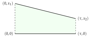
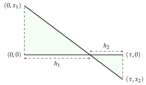
Figure 1: Area between two line segments: the two alternatives

We consider two cases.

Case 1: $x_{1}x_{2}\geq 0$. Then it is obvious that

(31) $$A(x_{1},x_{2})=\frac{\tau}{2}\big{(}|x_{1}|+|x_{2}|\big{)}.$$

Case 2: $x_{1}x_{2}<0$. Then the area consists of two triangles (see Figure 1) with heights

(32) $$h_{1}=\frac{|x_{1}|\tau}{|x_{1}|+|x_{2}|}\quad\text{and}\quad h_{2}=\frac{|x_{2}|\tau}{|x_{1}|+|x_{2}|}.$$

Therefore,

(33) $$A(x_{1},x_{2})=\frac{h_{1}|x_{1}|}{2}+\frac{h_{2}|x_{2}|}{2}=\frac{\tau}{2}\Big{(}\frac{x_{1}^{2}+x_{2}^{2}}{|x_{1}|+|x_{2}|}\Big{)}.$$

Combining these two possibilities, we find that

(34) $$A(x_{1},x_{2})=\begin{cases}\displaystyle\frac{\tau}{2}\bigg{(}\frac{x_{1}^{2}+x_{2}^{2}+2\max\{0,x_{1}x_{2}\}}{|x_{1}|+|x_{2}|}\bigg{)},&\text{if}\quad(x_{1},x_{2})\neq(0,0);\\ 0,&\text{otherwise}.\end{cases}$$

Because $\tau$ is fixed, our interest will be in the following function:

Definition 3.1 (stadium norm)

The stadium norm is defined by

(35) $$f:\mathbb{R}^{2}\to\mathbb{R}:(x_{1},x_{2})\mapsto\begin{cases}\displaystyle\frac{x_{1}^{2}+x_{2}^{2}+2\max\{0,x_{1}x_{2}\}}{|x_{1}|+|x_{2}|},&\text{if}\quad(x_{1},x_{2})\neq(0,0);\\ 0,&\text{otherwise}.\end{cases}$$

In fact, one can check that for every $\alpha>0$, the level set $\big{\{}{x\in\mathbb{R}^{2}}~{}\big{|}~{}{f(x)=\alpha}\big{\}}$ has the geometric shape of a stadium (see Figure 2). This motivates the name “stadium norm”; for the formal proof that $f$ is indeed a norm, see Section 4 below.

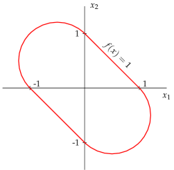
Figure 2: A level set of the stadium norm.

3.2 Upper approximations of the area

Since working with the true area (34) can be challenging (see Section 5.2 below), we are also interested in simpler approximations. Using the setting of Figure 1, we consider two approximations: the classical $\ell^{1}$-approximation

(36) $$A^{\ell}(x)=\frac{\tau}{2}\ell(x)\quad\text{where}\quad\ell(x):=\|x\|_{1}=|x_{1}|+|x_{2}|;$$

and the hexagonal stadium approximation

(37) $$A^{\ell}(x)=\frac{\tau}{2}h(x_{1},x_{2})\quad\text{where}\quad h(x_{1},x_{2}):=\max\big{\{}|x_{1}|,|x_{2}|,|x_{1}+x_{2}|\big{\}}.$$

Both $A^{\ell}$ and $A^{\rm h}$ are upper approximations, overestimating the true area $A$: $A^{\ell}\geq A^{\rm h}\geq A$ (see Figure 3).

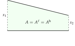
(a) $x_{1}x_{2}\geq 0$

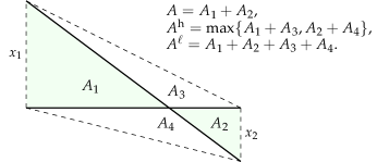
(b) $x_{1}x_{2}<0$

Figure 3: $A^{\ell}$ and $A^{\rm h}$ are upper approximations for the area $A$.

In fact, the relationships among $A^{\ell}$, $A^{\rm h}$, and $A$ reflect those among $f$, $\ell$, and $h$, which we turn to now:

Lemma 3.2 (upper approximations of the stadium norm)

Consider the stadium norm $f$ from (35), the norm $\ell=\|\cdot\|_{1}$ from (36), and the hexagonal stadium norm $h$ from (37). Let $x=(x_{1},x_{2})\in\mathbb{R}^{2}$. Then

(38a) $$f(x)\leq h(x)\leq\ell(x)$$

and

(38b) $$f(x)=h(x)=\ell(x)\quad\Leftrightarrow\quad x_{1}x_{2}\geq 0.$$

Moreover,

(39) $$\ell(x)-f(x)\geq 2\big{(}h(x)-f(x)\big{)}$$

and the constant $2$ is optimal.

Proof. (38a): The second inequality is clear. To prove the first one, we consider two cases. Case 1: $x_{1}x_{2}\geq 0$. Then $f(x)=|x_{1}|+|x_{2}|=|x_{1}+x_{2}|=\max\{|x_{1}|,|x_{2}|,|x_{1}+x_{2}|\}=h(x)=\ell(x)$. Case 2: $x_{1}x_{2}<0$. Then $f(x)=\tfrac{x_{1}^{2}+x_{2}^{2}}{|x_{1}|+|x_{2}|}\leq\max\{|x_{1}|,|x_{2}|\}\leq h(x)$.

(38b): This follows easily from the definitions.

(39): In view of (38b), the inequality is trivial when $x_{1}x_{2}\geq 0$. Thus, we assume that $x_{1}x_{2}<0$. Set $M:=\max\{|x_{1}|,|x_{2}|\}$ and $m:=\min\{|x_{1}|,|x_{2}|\}$. Then $f(x)=(m^{2}+M^{2})/(m+M)$, $h(x)=M$ and $\ell(x)=m+M$. Hence if $\beta\in\mathbb{R}_{++}$, then

(40) $$\ell(x)-f(x)=m+M-\frac{m^{2}+M^{2}}{m+M}=\frac{2mM}{m+M}$$

and

(41) $$\beta\big{(}h(x)-f(x)\big{)}=\beta\bigg{(}M-\frac{m^{2}+M^{2}}{m+M}\bigg{)}=\frac{\beta m(M-m)}{m+M}.$$

This implies (39) and we also conclude that the constant $2$ is optimal. $\hfill\quad\blacksquare$

3.3 The signed area between two line segments

We will now derive a formula for the signed area $S_{\tau}(x_{1},x_{2})$ between two line segments $[(0,0),(\tau,0)]$ and $[(0,x_{1}),(\tau,x_{2})]$ (see Figure 4). Consider, e.g., the case when $x_{1}>0$ and $x_{2}<0$. Using (32), we have

(42) $$S_{\tau}(x_{1},x_{2})=\frac{h_{1}|x_{1}|}{2}-\frac{h_{2}|x_{2}|}{2}=\frac{\tau}{2}\frac{x_{1}^{2}-x_{2}^{2}}{|x_{1}|+|x_{2}|}=\frac{\tau}{2}\big{(}|x_{1}|-|x_{2}|\big{)}=\frac{\tau}{2}(x_{1}+x_{2}).$$

The remaining cases can be dealt with analogously; altogether, we then obtain the following simple formula for the signed area between the two line segments:

(43) $$S_{\tau}(x_{1},x_{2})=\frac{\tau}{2}(x_{1}+x_{2}).$$

Figure 4: Signed area between the two line segments

4 The stadium norm and its approximations

We now justify our naming convention by showing that the stadium norm is actually a norm. (For further recent results on checking convexity of piecewise-defined functions, see [5].)

Theorem 4.1 (stadium norm is indeed a norm)

Set

(44) $$f\colon\mathbb{R}^{2}\to\mathbb{R}\colon(x_{1},x_{2})\mapsto\begin{cases}\displaystyle\frac{x_{1}^{2}+x_{2}^{2}+2\max\{0,x_{1}x_{2}\}}{|x_{1}|+|x_{2}|},&\text{if $(x_{1},x_{2})\neq(0,0)$;}\\ 0,&\text{otherwise,}\end{cases}$$

and let $\Omega_{1}=\mathbb{R}_{+}\times\mathbb{R}_{+}$, $\Omega_{2}=\mathbb{R}_{-}\times\mathbb{R}_{+}$, $\Omega_{3}=\mathbb{R}_{-}\times\mathbb{R}_{-}$, and $\Omega_{4}=\mathbb{R}_{+}\times\mathbb{R}_{-}$ denote the four closed quadrants in the Euclidean plane. Then $f$ is a norm, called the stadium norm, and continuously differentiable at every point $(x_{1},x_{2})\in\mathbb{R}^{2}\smallsetminus\{(0,0)\}$ with

(45) $$\nabla f(x_{1},x_{2})=\begin{cases}(1,1),&\text{if $(x_{1},x_{2})\in\Omega_{1}$;}\\[5.69054pt] \displaystyle\bigg{(}\frac{-x_{1}^{2}+2x_{1}x_{2}+x_{2}^{2}}{(x_{1}-x_{2})^{2}},\frac{-x_{1}^{2}-2x_{1}x_{2}+x_{2}^{2}}{(x_{1}-x_{2})^{2}}\bigg{)},&\text{if $(x_{1},x_{2})\in\Omega_{2}$;}\\[5.69054pt] (-1,-1),&\text{if $(x_{1},x_{2})\in\Omega_{3}$;}\\[5.69054pt] \displaystyle\bigg{(}\frac{x_{1}^{2}-2x_{1}x_{2}-x_{2}^{2}}{(x_{1}-x_{2})^{2}},\frac{x_{1}^{2}+2x_{1}x_{2}-x_{2}^{2}}{(x_{1}-x_{2})^{2}}\bigg{)},&\text{if $(x_{1},x_{2})\in\Omega_{4}$.}\end{cases}$$

Proof. It is clear that $f$ is continuous and that $f$ is positively homogeneous. The identity (45) follows easily from the definition of $f$. Let $x=(x_{1},x_{2})\in\mathbb{R}^{2}\smallsetminus\{(0,0)\}$. If $x\in\Omega_{1}\cup\Omega_{3}$, then $f(x)=|x_{1}|+|x_{2}|$; thus, $f|_{\Omega_{1}}$ and $f|_{\Omega_{3}}$ are obviously convex. If $x\in\operatorname{int}\Omega_{2}$, then the Hessian of $f$ at $x$,

(46) $$\nabla^{2}f(x)=\frac{4}{(x_{2}-x_{1})^{3}}\begin{pmatrix}x_{2}^{2}&-x_{1}x_{2}\\ -x_{1}x_{2}&x_{1}^{2}\end{pmatrix},$$

is positive semidefinite. It follows that $f|_{\operatorname{int}\Omega_{2}}$ is convex and so is $f|_{\Omega_{2}}$ by using the continuity of $f$ (see, e.g., [2, Proposition 17.10 and Proposition 9.26]). The proof of the convexity of $f|_{\Omega_{4}}$ is similar.

Now let $y\in\mathbb{R}^{2}$ and assume that $(0,0)\notin[x,y]$. Then there exist points (not necessarily distinct) points $u$ and $v$ in $\mathbb{R}^{2}$ such that

(47) $$[x,y]=[x,u]\cup[u,v]\cup[v,y],$$

with $[x,u]\subseteq A_{1}$, $[u,v]\subseteq A_{2}$, and $[v,y]\subseteq A_{3}$, where $\{A_{1},A_{2},A_{3}\}\subseteq\{\Omega_{1},\Omega_{2},\Omega_{3},\Omega_{4}\}$. Note that $f$ is differentiable on $[x,y]$. We claim that

(48) $$\left\langle{\nabla f(x)},{y-u}\right\rangle\leq\left\langle{\nabla f(u)},{y-u}\right\rangle.$$

Indeed, (48) is obvious when $x=u$. If $u\neq x$, then, since $f$ is convex in $A_{1}$, we have

(49a) $$\left\langle{\nabla f(x)},{y-u}\right\rangle =\tfrac{\|y-u\|}{\|u-x\|}\left\langle{\nabla f(x)},{u-x}\right\rangle$$

(49b) $$\leq\tfrac{\|y-u\|}{\|u-x\|}\left\langle{\nabla f(u)},{u-x}\right\rangle=\left\langle{\nabla f(u)},{y-u}\right\rangle.$$

Analogously, we see that

(50) $$\left\langle{\nabla f(u)},{y-v}\right\rangle\leq\left\langle{\nabla f(v)},{y-v}\right\rangle.$$

Employing (48), (50), and the convexity of $f|_{A_{i}}$, we deduce

(51a) $$\left\langle{\nabla f(x)},{y-x}\right\rangle =\left\langle{\nabla f(x)},{u-x}\right\rangle+\left\langle{\nabla f(x)},{y-u}\right\rangle$$

(51b) $$\leq f(u)-f(x)+\left\langle{\nabla f(u)},{y-u}\right\rangle$$

(51c) $$=f(u)-f(x)+\left\langle{\nabla f(u)},{v-u}\right\rangle+\left\langle{\nabla f(u)},{y-v}\right\rangle$$

(51d) $$\leq\big{(}f(u)-f(x)\big{)}+\big{(}f(v)-f(u)\big{)}+\left\langle{\nabla f(v)},{y-v}\right\rangle$$

(51e) $$\leq\big{(}f(v)-f(x)\big{)}+\big{(}f(y)-f(v)\big{)}$$

(51f) $$=f(y)-f(x).$$

To summarize, we have proven

(52) $$(0,0)\notin[x,y]\;\;\Rightarrow\;\;\left\langle{\nabla f(x)},{y-x}\right\rangle\leq f(y)-f(x).$$

Now let $x$ and $y$ be in $\mathbb{R}^{2}$ such that $x\neq y$, let $\lambda\in[0,1]$, and set $z=(1-\lambda)x+\lambda y$. It remains to show that

(53) $$f(z)\leq(1-\lambda)f(x)+\lambda f(y).$$

Case 1: $(0,0)\notin[x,y]$.
Then $(0,0)\notin[x,z]$ and $(0,0)\notin[z,y]$. Applying (52) twice, we obtain

(54) $$\left\langle{\nabla f(z)},{x-z}\right\rangle\leq f(x)-f(z)\quad\text{and}\quad\left\langle{\nabla f(z)},{y-z}\right\rangle\leq f(y)-f(z).$$

It follows that $(1-\lambda)\left\langle{\nabla f(z)},{x-z}\right\rangle\leq(1-\lambda)(f(x)-f(z))$ and $\lambda\left\langle{\nabla f(z)},{y-z}\right\rangle\leq\lambda(f(y)-f(z))$, which after adding and re-arranging turns into (53).

Case 2: $(0,0)\in[x,y]$.
Let $w$ be a unit vector perpendicular to $[x,y]$, let $\varepsilon\in\mathbb{R}_{++}$, and set

(55) $$x_{\varepsilon}=x+\varepsilon w,\;\;y_{\varepsilon}=y+\varepsilon w,\;\;\text{and}\;\;z_{\varepsilon}=z+\varepsilon w.$$

It is clear that $(0,0)\not\in[x_{\varepsilon},y_{\varepsilon}]$. So, applying Case 1 to $[x_{\varepsilon},y_{\varepsilon}]$, we deduce that

(56) $$f(z_{\varepsilon})\leq(1-\lambda)f(x_{\varepsilon})+\lambda f(y_{\varepsilon}).$$

Taking the limit as $\varepsilon\to 0^{+}$ and using the continuity of $f$, we obtain (53). $\hfill\quad\blacksquare$

Proposition 4.2 (dual stadium norm)

Consider the norm

(57) $$g\colon\mathbb{R}^{2}\to\mathbb{R}\colon(x_{1},x_{2})\mapsto\tfrac{1}{2}|x_{1}-x_{2}|+\tfrac{1}{\sqrt{2}}\|(x_{1},x_{2})\|.$$

Then the stadium norm $f$ given by (44) is the norm dual to $g$.

Proof. Let us sketch the derivation. It is easy to check that $g$ is indeed a norm. Denote the norm dual to $g$ by $g_{*}$. By If $g(\xi,\eta)=1$, then solving for $\eta$ yields two solutions, namely

(58) $$\eta_{\pm}(\xi)=-\xi\pm 2\big{(}\sqrt{2\pm 2\xi}-1\big{)},\;\;\text{where $\xi\in[-1,1]$}.$$

Now let $(x_{1},x_{2})\in\mathbb{R}^{2}$. Hence, using (25), we have

(59a) $$g_{*}(x_{1},x_{2}) =\sup\big{\{}{x_{1}\xi+x_{2}\eta}~{}\big{|}~{}{g(\xi,\eta)=1}\big{\}}$$

(59b) $$=\max\Big{\{}\max_{\xi\in[-1,1]}\big{(}x_{1}\xi+x_{2}\eta_{+}(\xi)\big{)},\max_{\xi\in[-1,1]}\big{(}x_{1}\xi+x_{2}\eta_{-}(\xi)\big{)}\Big{\}}.$$

This reduces the problem to one-dimensional calculus. If $x_{1}\neq x_{2}$, then the the critical points of the functions $\xi\mapsto x_{1}\xi+x_{2}\eta_{+}(\xi)$ and $\xi\mapsto x_{1}\xi+x_{2}\eta_{-}(\xi)$ are $\mp(x_{1}^{2}-2x_{1}x_{2}+x_{2}^{2})/(x_{1}-x_{2})^{2}$; otherwise the critical points are the endpoints $\mp 1$. Substituting the critical points into (59) yields indeed $g_{*}=f$. $\hfill\quad\blacksquare$

Let us summarize our finding in the following result:

Theorem 4.3 (the three norms)

The following table summarizes the dual norms found for the three planar norms of interest (see also Figure 5).

Norm $f$	Formula for $f(x)$	Formula for $f_{*}(x)$
$\ell=\|\cdot\|_{1}$	$|x_{1}|+|x_{2}|$.	$\max\big{\{}|x_{1}|,|x_{2}|\big{\}}$
hexagonal stadium	$\max\big{\{}|x_{1}|,|x_{2}|,|x_{1}+x_{2}|\big{\}}$	$\max\big{\{}|x_{1}|,|x_{2}|,|x_{1}-x_{2}|\big{\}}$
stadium	$\displaystyle\frac{x_{1}^{2}+x_{2}^{2}+2\max\{0,x_{1}x_{2}\}}{|x_{1}|+|x_{2}|}$	$\tfrac{1}{2}|x_{1}-x_{2}|+\tfrac{1}{\sqrt{2}}\|(x_{1},x_{2})\|$

Proof. Case 1: $f=\ell=\|\cdot\|_{1}$.
Of course, this case is well known, we include the details because it is short and for completeness. Note that its unit ball is $\operatorname*{conv}\{\pm(1,0),\pm(0,1)\}$. Again (26) yields

(60a) $$f_{*}(u_{1},u_{2}) =\max\big{\{}{u_{1}x_{1}+u_{2}x_{2}}~{}\big{|}~{}{(x_{1},x_{2})\in\{\pm(1,0),\pm(0,1)\}}\big{\}}$$

(60b) $$=\max\big{\{}\pm u_{1},\pm u_{2}\big{\}}$$

(60c) $$=\max\big{\{}|u_{1}|,|u_{2}|\big{\}}$$

(60d) $$=\|(u_{1},u_{2})\|_{\infty}.$$

Case 2: Hexagonal stadium norm.
Here $f(x)=\max\{|x_{1}|,|x_{2}|,|x_{1}+x_{2}|\}$. Considering the unit sphere $f(x)=1$, we compute that the unit ball is $\operatorname*{conv}\{\pm(-1,1),\pm(1,0),\pm(0,1)\}$. Now let $(u_{1},u_{2})\in\mathbb{R}^{2}$. It follows from (26) that

(61a) $$f_{*}(u_{1},u_{2}) =\max\big{\{}{u_{1}x_{1}+u_{2}x_{2}}~{}\big{|}~{}{(x_{1},x_{2})\in\{\pm(-1,1),\pm(1,0),\pm(0,1)\}}\big{\}}$$

(61b) $$=\max\big{\{}\pm(u_{2}-u_{1}),\pm u_{1},\pm u_{2}\big{\}}$$

(61c) $$=\max\big{\{}|u_{1}|,|u_{2}|,|u_{1}-u_{2}|\big{\}}.$$

Case 3: $f$ is the stadium norm — see Theorem 4.1 and Proposition 4.2. $\hfill\quad\blacksquare$

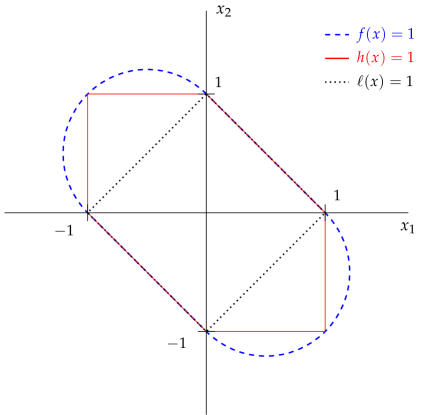
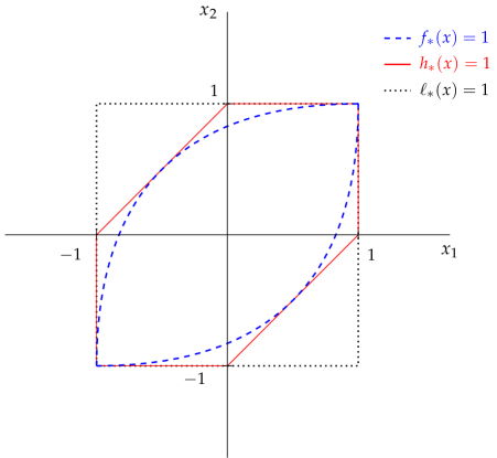
Figure 5: Primal and dual balls of the stadium norm $f$, the hexagonal stadium norm $h$, and classical $\ell=\|\cdot\|_{1}$.

5 Proximity operators of some planar norms

5.1 Projectors onto the dual balls for two polyhedral norms

The following result is well known.

Proposition 5.1 (dual $\|\cdot\|_{1}$ ball projector)

Let $\|\cdot\|_{1}\colon(x_{1},x_{2})\to|x_{1}|+|x_{2}|$ be the $\ell^{1}$ norm on $\mathbb{R}^{2}$, denote its dual ball $[-1,1]\times[-1,1]$ by $B_{*}$, and let $x=(x_{1},x_{2})\in\mathbb{R}^{2}$. Then

(62) $$\operatorname{P}_{B_{*}}(x_{1},x_{2})=\big{(}\operatorname{P}_{[-1,1]}(x_{1}),\operatorname{P}_{[-1,1]}(x_{1})\big{)}.$$

Proposition 5.2 (dual hexagonal stadium ball projector)

Let $(x_{1},x_{2})\mapsto\max\{|x_{1}|,|x_{2}|,|x_{1}+x_{2}|\}$ be the hexagonal stadium norm, denote its dual ball by $B_{*}$, and let $x=(x_{1},x_{2})\in\mathbb{R}^{2}$. Then

(63) $$\operatorname{P}_{B_{*}}(x)=\begin{cases}x,&\text{if $x\in B_{*}$;}\\ \big{(}\operatorname{P}_{[0,1]}(x_{1}),\operatorname{P}_{[0,1]}(x_{2})\big{)},&\text{if $(x_{1},x_{2})\in(\mathbb{R}_{+}\times\mathbb{R}_{+})\smallsetminus B_{*}$;}\\ \operatorname{P}_{[(-1,0),(0,1)]}(x),&\text{if $(x_{1},x_{2})\in(\mathbb{R}_{-}\times\mathbb{R}_{+})\smallsetminus B_{*}$;}\\ \big{(}\operatorname{P}_{[-1,0]}(x_{1}),\operatorname{P}_{[-1,0]}(x_{2})\big{)},&\text{if $(x_{1},x_{2})\in(\mathbb{R}_{-}\times\mathbb{R}_{-})\smallsetminus B_{*}$;}\\ \operatorname{P}_{[(0,-1),(1,0)]}(x),&\text{if $(x_{1},x_{2})\in(\mathbb{R}_{-}\times\mathbb{R}_{+})\smallsetminus B_{*}$.}\end{cases}$$

Alternatively (and better suited to programming), we have

(64) $$\operatorname{P}_{B_{*}}(x)=\begin{cases}x,&\text{if $f_{*}(x)\leq 1$;}\\ \big{(}\operatorname{P}_{[-1,1]}(x_{1}),\operatorname{P}_{[-1,1]}(x_{2})\big{)},&\text{else if $x_{1}x_{2}\geq 0$;}\\ \operatorname{sgn}(x_{1})\big{(}\tfrac{1}{2},-\tfrac{1}{2}\big{)}+\operatorname{P}_{[-1,1]}(x_{1}+x_{2})\big{(}\tfrac{1}{2},\tfrac{1}{2}\big{)},&\text{else.}\end{cases}$$

Proof. Formula (63) follows from observing that

(65) $$B_{*}=\operatorname*{conv}\big{\{}\pm(1,0),\pm(0,1),\pm(1,1)\big{\}},$$

and by considering each quadrant. To obtain (64), consider cases and use (9). $\hfill\quad\blacksquare$

5.2 Projector onto the dual ball of the stadium norm

In this section, we derive the projector onto the dual ball of the stadium norm. This will require significantly more work than the two polyhedral norms just discussed. We start by setting

(66a) $$\Gamma_{0}\colon\big{[}-\tfrac{\pi}{2},0\big{]} \to\mathbb{R}^{2}$$

(66b) $$t \mapsto\Big{(}\frac{\cos^{2}t-2\sin t\cos t-\sin^{2}t}{(\cos t-\sin t)^{2}},\frac{\cos^{2}t+2\sin t\cos t-\sin^{2}t}{(\cos t-\sin t)^{2}}\Big{)}.$$

and

(67) $$R=\operatorname{ran}\Gamma_{0}.$$

In view of Lemma 2.4 and (45), it follows that

(68) $$B_{*}=\operatorname*{conv}\big{(}R\cup(-R)\big{)}.$$

Using trigonometric identities, we see that for every $t\in[-\pi/2,0]$ we have

(69) $$\Gamma_{0}(t)=\Big{(}\frac{\cos 2t-\sin 2t}{1-\sin 2t},\frac{\cos 2t+\sin 2t}{1-\sin 2t}\Big{)}=\Big{(}\frac{\sqrt{2}\cos(2t+\frac{\pi}{4})}{1-\sin 2t},\frac{\sqrt{2}\sin(2t+\frac{\pi}{4})}{1-\sin 2t}\Big{)}.$$

By changing variables, we thus see that

(70a) $$\Gamma_{1}\colon\big{[}-\tfrac{3\pi}{4},\tfrac{\pi}{4}\big{]} \to\mathbb{R}^{2}$$

(70b) $$t \mapsto\Big{(}\frac{\sqrt{2}\cos t}{1-\sin(t-\pi/4)},\frac{\sqrt{2}\sin t}{1-\sin(t-\pi/4)}\Big{)}$$

(70c) $$=\frac{\sqrt{2}}{1+\cos(t+\pi/4)}\big{(}\cos t,\sin t\big{)}$$

satisfies

(71) $$R=\operatorname{ran}\Gamma_{1}.$$

In polar coordinates $(r,\omega)$, the parametrizations of $\Gamma_{1}$ and $-\Gamma_{1}$ become

(72a) $$(\Gamma_{1}) :\quad r=\frac{\sqrt{2}}{1+|\cos(\omega+\pi/4)|}=\frac{\sqrt{2}}{1+\cos(\omega+\pi/4)},\quad\omega\in\big{[}-\tfrac{3\pi}{4},\tfrac{\pi}{4}\big{]};$$

(72b) $$(-\Gamma_{1}) :\quad r=\frac{\sqrt{2}}{1+|\cos(\omega+\pi/4)|}=\frac{\sqrt{2}}{1-\cos(\omega+\pi/4)},\quad\omega\in\big{[}\tfrac{\pi}{4},\tfrac{5\pi}{4}\big{]}.$$

Now set

(73a) $$A_{1} :=\big{\{}{(x_{1},x_{2})\in\mathbb{R}^{2}}~{}\big{|}~{}{x_{1}\geq 1,x_{2}\geq 1}\big{\}},$$

(73b) $$A_{2} :=\big{\{}{(x_{1},x_{2})\in\mathbb{R}^{2}}~{}\big{|}~{}{x_{1}>-1,x_{2}<1,x_{2}<x_{1}}\big{\}}.$$

Then, for every $x=(r\cos\omega,r\sin\omega)\in\mathbb{R}^{2}$, we have

(74) $$P_{B_{*}}(x)=\begin{cases}(1,1),&\text{if $x\in A_{1}$;}\\[5.69054pt] (-1,-1),&\text{if $x\in-A_{1}$;}\\[5.69054pt] x,&\text{if $\displaystyle r\leq\frac{\sqrt{2}}{1+|\cos(\omega+\pi/4)|}$;}\\[5.69054pt] \operatorname{P}_{R}(x),&\text{if $x\in A_{2}$ ~{}and~{} $\displaystyle r>\frac{\sqrt{2}}{1+\cos(\omega+\pi/4)}$;}\\[5.69054pt] \operatorname{P}_{-R}(x)=-\operatorname{P}_{R}(-x),&\text{if $x\in-A_{2}$ ~{}and~{} $\displaystyle r>\frac{\sqrt{2}}{1-\cos(\omega+\pi/4)}$.}\end{cases}$$

For a sketch, see Figure 6.

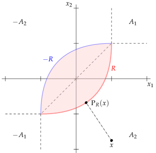
Figure 6: Projection onto the dual stadium ball

Now suppose that

(75) $$x\in A_{2}\;\;\text{and}\;\;r>\frac{\sqrt{2}}{1+\cos(\omega+\pi/4)}.$$

Since $x\in A_{2}$, we have $\omega\in\left]-3\pi/4,\pi/4\right[$ and thus $\cos(\omega+\pi/4)>0$. Denote the squared distance from $x=(r\cos\omega,r\sin\omega)$ to $\Gamma_{1}(t)$, where $t\in[-3\pi/4,\pi/4]$ (see (70a)) by

(76) $$F(t) =\Big{(}\tfrac{\sqrt{2}\cos t}{1+\cos(t+\pi/4)}-r\cos\omega\Big{)}^{2}+\Big{(}\tfrac{\sqrt{2}\sin t}{1+\cos(t+\pi/4)}-r\sin\omega\Big{)}^{2}$$

(77) $$=2\Big{(}\tfrac{\cos t}{1+\cos(t+\pi/4)}-\tfrac{r\cos\omega}{\sqrt{2}}\Big{)}^{2}+2\Big{(}\tfrac{\sin t}{1+\cos(t+\pi/4)}-\tfrac{r\sin\omega}{\sqrt{2}}\Big{)}^{2}$$

We now claim that

(78) $$\begin{cases}&\text{$F$ is a convex function on $[-3\pi/4,\pi/4]$, and}\\ &\text{$F^{\prime}(t)=0$ has a unique solution in $\left]-3\pi/4,\pi/4\right[$.}\end{cases}$$

The critical number $t$ will then yield the projection $P_{R}(x)=\Gamma_{1}(t)$. We start by computing the derivative of $F$: Indeed,

(79a) $$F^{\prime}(t) =4\Big{(}\tfrac{\cos t}{1+\cos(t+\pi/4)}-\tfrac{r\cos\omega}{\sqrt{2}}\Big{)}\tfrac{-\sin t(1+\cos(t+\pi/4))+\sin(t+\pi/4)\cos t}{(1+\cos(t+\pi/4))^{2}}$$

(79b) $$\quad+4\Big{(}\tfrac{\sin t}{1+\cos(t+\pi/4)}-\tfrac{r\sin\omega}{\sqrt{2}}\Big{)}\tfrac{\cos t(1+\cos(t+\pi/4))+\sin(t+\pi/4)\sin t}{(1+\cos(t+\pi/4))^{2}}$$

(79c) $$=4\Big{(}\tfrac{\cos t}{1+\cos(t+\pi/4)}-\tfrac{r\cos\omega}{\sqrt{2}}\Big{)}\tfrac{-\sin t+\sin(\pi/4)}{(1+\cos(t+\pi/4))^{2}}$$

(79d) $$\quad+4\Big{(}\tfrac{\sin t}{1+\cos(t+\pi/4)}-\tfrac{r\sin\omega}{\sqrt{2}}\Big{)}\tfrac{\cos t+\cos(\pi/4)}{(1+\cos(t+\pi/4))^{2}}$$

(79e) $$=\tfrac{4}{(1+\cos(t+\pi/4))^{2}}\Big{(}\tfrac{\sin(t+\pi/4)}{1+\cos(t+\pi/4)}+\tfrac{r(\sin(t-\omega)-\sin(\omega+\pi/4))}{\sqrt{2}}\Big{)}$$

Setting

(80) $$u:=t+\tfrac{\pi}{4}\in\left[-\tfrac{\pi}{2},\tfrac{\pi}{2}\right]\quad\text{and}\quad\theta:=\omega+\tfrac{\pi}{4}\in\left]-\tfrac{\pi}{2},\tfrac{\pi}{2}\right[,$$

we see that

(81a) $$F^{\prime}(t) =\tfrac{4}{1+\cos u}\Big{(}\tfrac{\sin u}{(1+\cos u)^{2}}+\tfrac{r}{\sqrt{2}}\tfrac{\sin(u-\theta)-\sin\theta}{(1+\cos u)}\Big{)}$$

(81b) $$=\tfrac{4}{1+\cos u}\Big{(}\tfrac{\sin u}{(1+\cos u)^{2}}+\tfrac{r}{\sqrt{2}}\tfrac{\sin u\cos\theta-\cos u\sin\theta-\sin\theta}{(1+\cos u)}\Big{)}$$

(81c) $$=\tfrac{4}{1+\cos u}\Big{(}\tfrac{\sin u}{(1+\cos u)^{2}}+\tfrac{r}{\sqrt{2}}\tfrac{\sin u\cos\theta}{(1+\cos u)}-\tfrac{r\sin\theta}{\sqrt{2}}\Big{)}.$$

Furthermore, set

(82) $$s:=\tan(u/2)\in[-1,1],\ \alpha:=\tfrac{r}{\sqrt{2}}\cos\theta>0,\ \text{and}\ \beta:=\tfrac{r}{\sqrt{2}}\sin\theta.$$

Then $\tfrac{1}{1+\cos u}=\tfrac{1}{2\cos^{2}(u/2)}=\tfrac{1+s^{2}}{2}$ and

(83) $$F^{\prime}(t) =\tfrac{4}{2\cos^{2}(u/2)}\Big{(}\tfrac{2\sin(u/2)\cos(u/2)}{4\cos^{4}(u/2)}+\tfrac{2\alpha\sin(u/2)\cos(u/2)}{2\cos^{2}(u/2)}-\beta\Big{)}$$

(84) $$=2(1+s^{2})\Big{(}\tfrac{1}{2}s(1+s^{2})+\alpha s-\beta\Big{)}$$

(85) $$=(1+s^{2})\big{(}s^{3}+(1+2\alpha)s-2\beta\big{)}.$$

Let

(86) $$G\colon[-1,1]\to\mathbb{R}\colon s\mapsto(1+s^{2})\big{(}s^{3}+(1+2\alpha)s-2\beta\big{)}$$

and consider the equation

(87) $$G(s)=0.$$

Since $x=(x_{1},x_{2})\in A_{2}$, we have $x_{1}=r\cos\omega>-1$ and $x_{2}=r\sin\omega<1$. Hence

(88a) $$\alpha-\beta =\tfrac{r}{\sqrt{2}}(\cos\theta-\sin\theta)=-r\sin\omega>-1,$$

(88b) $$\alpha+\beta =\tfrac{r}{\sqrt{2}}(\cos\theta+\sin\theta)=r\cos\omega>-1;$$

consequently,

(89) $$G(1)=2(2+2\alpha-2\beta)>0\quad\text{and}\quad G(-1)=2(-2-2\alpha-2\beta)<0.$$

Since $G$ is clearly continuous, it follows that (87) has a solution in $\left]-1,1\right[$. We now compute

(90) $$G^{\prime}(s)=5s^{4}+6(1+\alpha)s^{2}-4\beta s+(1+2\alpha)$$

and observe that the discriminant of the quadratic polynomial $6(1+\alpha)s^{2}-4\beta s+(1+2\alpha)$ is $\Delta:=16\beta^{2}-24(1+\alpha)(1+2\alpha)$. Because $|\beta|<1+\alpha<1+2\alpha$ (by (88)), it is clear that $\Delta<0$. Hence $6(1+\alpha)s^{2}-4\beta s+(1+2\alpha)>0$ and therefore $G^{\prime}$ is strictly positive on $\left]-1,1\right[$. We deduce that $G$ is strictly increasing on $[-1,1]$. So the solution of (87) is unique. In turn, this implies that $F^{\prime}$ strictly increases on $[-3\pi/4,\pi/4]$. It follows that $F$ is a convex function on $[-3\pi/4,\pi/4]$ and that $F^{\prime}(t)=0$ has a unique solution in $\left]-3\pi/4,\pi/4\right[$. Therefore, $F$ has a unique minimizer in $\left]-3\pi/4,\pi/4\right[$, which establishes our claim (78).

Now let $s$ be the unique solution of (87), which implies that $s$ is a real solution of

(91) $$s^{3}+(1+2\alpha)s-2\beta=0.$$

This real solution is unique because viewed as function in $s$, the derivate of the left-hand side of (91) is $3s^{2}+(1+2\alpha)>0$ since $\alpha>0$. Cardano’s formula gives

(92) $$\sqrt[3]{\beta+\sqrt{\beta^{2}+(\tfrac{1+2\alpha}{3})^{3}}}+\sqrt[3]{\beta-\sqrt{\beta^{2}+(\tfrac{1+2\alpha}{3})^{3}}}$$

as a solution to (91). This solution is a real number, again since $\alpha>0$. Hence $s$ is equal to (92). Let us summarize what we have found out so far: If

(93a) $$x=r(\cos\omega,\sin\omega)\in A_{2}\;\;\text{and}\;\;r>\frac{\sqrt{2}}{1+\cos(\omega+\pi/4)},$$

and

(93b) $$\alpha =\tfrac{r}{\sqrt{2}}\cos(\omega+\pi/4),\;\;\beta=\tfrac{r}{\sqrt{2}}\sin(\omega+\pi/4),$$

(93c) $$s =\sqrt[3]{\beta+\sqrt{\beta^{2}+(\tfrac{1+2\alpha}{3})^{3}}}+\sqrt[3]{\beta-\sqrt{\beta^{2}+(\tfrac{1+2\alpha}{3})^{3}}}\ \in\left]-1,1\right[,$$

(93d) $$t =2\arctan(s)-\tfrac{\pi}{4}\in\left]-\tfrac{3\pi}{4},\tfrac{\pi}{4}\right[,$$

then

(93e) $$P_{R}(x)=\frac{\sqrt{2}}{1+\cos(t+\pi/4)}(\cos t,\sin t).$$

Our next goal is to simplify (93) by eliminating the trigonometric functions. To this end, let $(x_{1},x_{2})=r(\cos\omega,\sin\omega)\in A_{2}$. We translate (93) to a form that is free of trigonometric functions. Observe first that

(94a) $$r\cos(\omega+\pi/4)=\tfrac{1}{\sqrt{2}}r\cos\omega-\tfrac{1}{\sqrt{2}}r\sin\omega=\tfrac{1}{\sqrt{2}}(x_{1}-x_{2})>0$$

(94b) and $$r\sin(\omega+\pi/4)=\tfrac{1}{\sqrt{2}}r\cos\omega+\tfrac{1}{\sqrt{2}}r\sin\omega=\tfrac{1}{\sqrt{2}}(x_{1}+x_{2}).$$

Hence (93b) turns into

(95) $$\alpha=\tfrac{1}{2}(x_{1}-x_{2})\;\;\text{and}\;\;\beta=\tfrac{1}{2}(x_{1}+x_{2}).$$

Furthermore, since

(96) $$\frac{\sqrt{2}}{r\big{(}1+\cos(\omega+\pi/4)\big{)}}=\frac{\sqrt{2}}{r+r\cos(\omega+\pi/4)}=\frac{2}{\sqrt{2(x_{1}^{2}+x_{2}^{2})}+x_{1}-x_{2}},$$

we see that the inequality in (93a) is equivalent to

(97) $$\sqrt{2(x_{1}^{2}+x_{2}^{2})}+x_{1}-x_{2}>2.$$

Next, let $s$ and $t$ be as in (93c)–(93d). Using

(98) $$\cos(\arctan s)=\frac{1}{\sqrt{1+s^{2}}}\quad\text{and}\quad\sin(\arctan s)=\frac{s}{\sqrt{1+s^{2}}},$$

we have

(99a) $$\cos(t+\pi/4) =\cos(2\arctan s)=\cos^{2}(\arctan s)-\sin^{2}(\arctan s)=\frac{1-s^{2}}{1+s^{2}},$$

(99b) $$\sin(2\arctan s) =2\sin(\arctan s)\cos(\arctan s)=\frac{2s}{1+s^{2}}.$$

It follows that

(100a) $$\cos t =\tfrac{1}{\sqrt{2}}\big{(}\cos(2\arctan s)+\sin(2\arctan s)\big{)}=\frac{1+2s-s^{2}}{\sqrt{2}(1+s^{2})},$$

(100b) $$\sin t =\tfrac{1}{\sqrt{2}}\big{(}\sin(2\arctan s)-\cos(2\arctan s)\big{)}=\frac{-1+2s+s^{2}}{\sqrt{2}(1+s^{2})}.$$

Finally, (93e) turns into

(101) $$\operatorname{P}_{R}(x)=\frac{\sqrt{2}}{1+\tfrac{1-s^{2}}{1+s^{2}}}\bigg{(}\frac{1+2s-s^{2}}{\sqrt{2}(1+s^{2})},\frac{-1+2s+s^{2}}{\sqrt{2}(1+s^{2})}\bigg{)}=\bigg{(}\frac{1+2s-s^{2}}{2},\frac{-1+2s+s^{2}}{2}\bigg{)}.$$

Since $\operatorname{P}_{-R}(x)=-\operatorname{P}_{R}(-x)$, we can handle the case when $-x\in A_{2}$ analogously.

We are now in a position to summarize this section in the following result:

Theorem 5.3 (dual stadium ball projector)

Let

(102) $$f\colon\mathbb{R}^{2}\to\mathbb{R}\colon(x_{1},x_{2})\mapsto\begin{cases}\displaystyle\frac{x_{1}^{2}+x_{2}^{2}+2\max\{0,x_{1}x_{2}\}}{|x_{1}|+|x_{2}|},&\text{if $(x_{1},x_{2})\neq(0,0)$;}\\ 0,&\text{otherwise,}\end{cases}$$

be the stadium norm, denote its dual ball by $B_{*}$, and let $x=(x_{1},x_{2})\in\mathbb{R}^{2}$. Set

(103a) $$\alpha:=\tfrac{1}{27}\big{(}1+|x_{1}-x_{2}|\big{)}^{3},\;\;\beta:=\tfrac{1}{2}\operatorname{sgn}(x_{1}-x_{2})(x_{1}+x_{2}),$$

and

(103b) $$s:=\sqrt[3]{\beta+\sqrt{\beta^{2}+\alpha}}+\sqrt[3]{\beta-\sqrt{\beta^{2}+\alpha}}.$$

Then

(104) $$\operatorname{P}_{B_{*}}(x)=\begin{cases}(1,1),&\text{if $x_{1}\geq 1$ and $x_{2}\geq 1$;}\\ (-1,-1),&\text{if $x_{1}\leq-1$ and $x_{2}\leq-1$;}\\ (x_{1},x_{2}),&\text{if $\sqrt{2(x_{1}^{2}+x_{2}^{2})}+|x_{1}-x_{2}|\leq 2$;}\\ \displaystyle\operatorname{sgn}(x_{1}-x_{2})\bigg{(}\frac{1+2s-s^{2}}{2},\frac{-1+2s+s^{2}}{2}\bigg{)},&\text{otherwise.}\end{cases}$$

5.3 Proximity operators

Combining Lemma 2.6 with the formulae derived with in (62), (63)–(64), and (104), we are now able to summarize the findings of this section.

Theorem 5.4 (planar proximity operators)

Let $f\colon\mathbb{R}^{2}\to\mathbb{R}$ be a norm, and denote its dual ball by $B_{*}$. Let $\alpha$ and $\gamma$ be in $\mathbb{R}_{++}$, let $w\in X$, and set $h\colon X\to\mathbb{R}\colon x\mapsto\alpha f(x-w)$. Then

(105) $$(\forall x\in X)\quad\operatorname{P}_{\gamma h}(x)=x-\gamma\alpha\operatorname{P}_{B_{*}}(\tfrac{x-w}{\gamma\alpha})\quad\text{and}\quad\operatorname{P}_{\gamma h^{*}}(x)=\alpha\operatorname{P}_{B_{*}}(\tfrac{x-\gamma w}{\alpha}).$$

Let $x\in\mathbb{R}^{2}\smallsetminus\{(0,0)\}$. The following table summarizes several choices that will be used later.

Norm $f$	Formula for $f(x)$	Formula for $\operatorname{P}_{B_{*}}(x)$
$\ell=\|\cdot\|_{1}$	$|x_{1}|+|x_{2}|$.	see (62)
hexagonal stadium	$\max\big{\{}|x_{1}|,|x_{2}|,|x_{1}+x_{2}|\big{\}}$	see (63) or (64)
stadium	$\displaystyle\frac{x_{1}^{2}+x_{2}^{2}+2\max\{0,x_{1}x_{2}\}}{|x_{1}|+|x_{2}|}$	see (104)

6 Proximity operators in $\mathbb{R}^{n}$ related to area

Let

(106) $$t=(t_{1},\ldots,t_{n})\in X=\mathbb{R}^{n}\quad\text{such that}\quad t_{1}<\cdots<t_{n}.$$

Fix $w=(w_{1},\ldots,w_{n})\in X$ and let $x=(x_{1},\ldots,x_{n})\in X$. In this section, we first develop a formula for the area between the two linear splines $l_{(t,x)}$ and $l_{(t,w)}$ (see (3)) and then provide related proximity operators. We set

(107a) $$\tau_{i}:=(t_{i+1}-t_{i})/2\quad\text{for}\quad i\in\{1,\ldots,n-1\};$$

(107b) $$\eta:=(\eta_{1},\ldots,\eta_{n})\in X\quad\text{where}\quad\left\{\begin{aligned} &\eta_{1}:=\tau_{1};\quad\eta_{n}:=\tau_{n-1};\quad\text{and}\\ &\eta_{i}:=\tau_{i-1}+\tau_{i}\quad\text{for}\quad i\in\{2,\ldots,n-1\}.\end{aligned}\right.$$

6.1 Area between two linear splines

Figure 7: Area between two linear splines

Using Section 3.1 and Section 3.2, we estimate the area between the two line segments $[(t_{i},x_{i}),(t_{i+1},x_{i+1})]$ and $[(t_{i},w_{i}),(t_{i+1},w_{i+1})]$ (see Figure 7) by

(108) $$A_{i}(x_{i},x_{i+1})=\tau_{i}\cdot f(x_{i}-w_{i},x_{i+1}-w_{i+1}),$$

where the value of $A_{i}$ depends on the norm $f$ as shown in the following table:

Norm $f$	Value of $A_{i}(x_{i},x_{i+1})$
$\ell=\|\cdot\|_{1}$	upper estimate of the area
hexagonal stadium	upper estimate of the area
stadium	exact area

Then the total (absolute) area between two linear splines $l_{(t,x)}$ and $l_{(t,w)}$ is estimated by

(109) $$A(x)=\sum_{i=1}^{n-1}A_{i}(x_{i},x_{i+1})=\sum_{i=1}^{n-1}\tau_{i}\cdot f(x_{i}-w_{i},x_{i+1}-w_{i+1}).$$

Next, we will compute the proximity operators for the area estimate $A(x)$. While we are able to explicitly compute the proximity operators for each term of $A$ (see Theorem 5.4), the overall sum $A$ does not appear to admit a simple formula. To deal with $A(x)$, we split it into two parts,

(110a) $$A_{\rm odd}(x) =\tau_{1}\cdot f(x_{1}-w_{1},x_{2}-w_{2})+\tau_{3}\cdot f(x_{3}-w_{3},x_{4}-w_{4})+\cdots$$

$$=\sum_{i\in\{1,\ldots,n-1\}\cap(1+2\mathbb{N})}\tau_{i}\cdot f(x_{i}-w_{i},x_{i+1}-w_{i+1}),$$

and

(110b) $$A_{\rm even}(x) =\tau_{2}\cdot f(x_{2}-w_{2},x_{3}-w_{3})+\tau_{4}\cdot f(x_{4}-w_{4},x_{5}-w_{5})+\cdots$$

$$=\sum_{i\in\{1,\ldots,n-1\}\cap(2\mathbb{N})}\tau_{i}\cdot f(x_{i}-w_{i},x_{i+1}-w_{i+1}),$$

so that

(111) $$A=A_{\rm odd}+A_{\rm even}.$$

As the functions in (110) are decoupled into independent pairs of real variables, the proximity operators can be computed in parallel. Thus, grouping

(112) $$X\ni(y_{1},\ldots,y_{n})=\Big{(}(y_{1},y_{2}),(y_{3},y_{4}),\cdots\Big{)}=\Big{(}y_{1},(y_{2},y_{3}),(y_{4},y_{5}),\cdots\Big{)},$$

and using Theorem 5.4, we obtain the following result:

Theorem 6.1 (proximity operators for area estimations)

Let $A_{i}$ be given by (108) for every $i\in\{1,\ldots,n-1\}$, where $f$ is as in the table below. Let $A_{\rm odd}$ and $A_{\rm even}$ be defined by (110), let $\gamma\in\mathbb{R}_{++}$, let $\alpha\in\mathbb{R}_{++}$, and let $x\in X$. Then the proximity operators of $A_{\rm odd}$ and $A_{\rm even}$ are

(113a) $$\operatorname{P}_{\gamma(\alpha A_{\rm odd})}(x)=\big{(}\operatorname{P}_{\gamma(\alpha A_{1})}(x_{1},x_{2}),\operatorname{P}_{\gamma(\alpha A_{3})}(x_{3},x_{4}),\ldots\big{)},$$

where the last entry in (113a) is $$x_{n} n$$ if is odd;

(113b) $$\operatorname{P}_{\gamma(\alpha A_{\rm odd})^{*}}(x)=\big{(}\operatorname{P}_{\gamma(\alpha A_{1})^{*}}(x_{1},x_{2}),\operatorname{P}_{\gamma(\alpha A_{3})^{*}}(x_{3},x_{4}),\ldots\big{)},$$

where the last entry in (113b) is $0$ if $n$ is odd;

(113c) $$\operatorname{P}_{\gamma(\alpha A_{\rm even})}(x)=\big{(}x_{1},\operatorname{P}_{\gamma(\alpha A_{2})}(x_{2},x_{3}),\operatorname{P}_{\gamma(\alpha A_{4})}(x_{4},x_{5}),\ldots\big{)},$$

where the last entry in (113c) is $$x_{n} n$$ if is even;

(113d) $$\operatorname{P}_{\gamma(\alpha A_{\rm even})^{*}}(x)=\big{(}0,\operatorname{P}_{\gamma(\alpha A_{2})^{*}}(x_{2},x_{3}),\operatorname{P}_{\gamma(\alpha A_{4})^{*}}(x_{4},x_{5}),\ldots\big{)},$$

where the last entry in (113d) is $0$ if $n$ is even. In these formulas,

(114a) $$\operatorname{P}_{\gamma(\alpha A_{i})}(x_{i},x_{i+1})=(x_{i},x_{i+1})-\gamma\alpha\tau_{i}\operatorname{P}_{B_{*}}(\tfrac{x_{i}-w_{i}}{\gamma\alpha\tau_{i}},\tfrac{x_{i+1}-w_{i+1}}{\gamma\alpha\tau_{i}});$$

(114b) and $$\operatorname{P}_{\gamma(\alpha A_{i})^{*}}(x_{i},x_{i+1})=\tau_{i}\operatorname{P}_{B_{*}}(\tfrac{x_{i}-\gamma w_{i}}{\alpha\tau_{i}},\tfrac{x_{i+1}-\gamma w_{i+1}}{\alpha\tau_{i}}),$$

where $B_{*}$ is the dual unit ball of the norm $f$.

Norm $f$	Formula for $f(z_{1},z_{2})$	Formula for $\operatorname{P}_{B_{*}}$
$\ell=\|\cdot\|_{1}$	$|z_{1}|+|z_{2}|$.	see (62)
hexagonal stadium	$\max\big{\{}|z_{1}|,|z_{2}|,|z_{1}+z_{2}|\big{\}}$	see (63) or (64)
stadium	$\displaystyle\frac{z_{1}^{2}+z_{2}^{2}+2\max\{0,z_{1}z_{2}\}}{|z_{1}|+|z_{2}|}$	see (104)

It turns out that if $f=\ell=\|\cdot\|_{1}$ is used for the estimate $A(x)$, then the proximity operators become simpler since all variables $x_{i}$ appear separately:

Theorem 6.2 (proximity operators for $\ell=\|\cdot\|_{1}$ area estimation)

Let $l_{(t,x)}$ and $l_{(t,w)}$ be linear splines (see (3)), let

(115) $$A(x)=\sum_{i=1}^{n-1}A_{i}(x_{i},x_{i+1})=\sum_{i=1}^{n-1}\tau_{i}\cdot(|x_{i}-w_{i}|+|x_{i+1}-w_{i+1}|)=\sum_{i=1}^{n}\eta_{i}|x_{i}-w_{i}|$$

be the $\ell=\|\cdot\|_{1}$ estimation of the area between them (see (107)), let $\gamma\in\mathbb{R}_{++}$, and let $\alpha\in\mathbb{R}_{++}$. Then

(116a) $$\big{(}\operatorname{P}_{\gamma(\alpha A)}(x)\big{)}_{i}=\begin{cases}x_{i}+\gamma(\alpha\eta_{i})\displaystyle\frac{w_{i}-x_{i}}{|w_{i}-x_{i}|},&\text{if $|w_{i}-x_{i}|>\gamma\alpha\eta_{i}$;}\\ w_{i},&\text{otherwise,}\end{cases}$$

and

(116b) $$\big{(}\operatorname{P}_{\gamma(\alpha A)^{*}}(x)\big{)}_{i}=\begin{cases}(\alpha\eta_{i})\displaystyle\frac{x_{i}-\gamma w_{i}}{|x_{i}-\gamma w_{i}|},&\text{if $|x_{i}-\gamma w_{i}|>\alpha\eta_{i}$;}\\ x_{i}-\gamma w_{i},&\text{otherwise.}\end{cases}$$

6.2 Signed area between two linear splines

Taking into account the signed area between two line segments (see Section 3.3 and Figure 8), we obtain the following function of $x$ for the signed area between two linear splines $l_{(t,x)}$ and $l_{(t,w)}$:

(117) $$S\colon X\to\mathbb{R}\colon x\mapsto\sum_{i=1}^{n-1}\tau_{i}\big{(}(x_{i}-w_{i})+(x_{i+1}-w_{i+1})\big{)}=\sum_{i=1}^{n}\eta_{i}(x_{i}-w_{i})=\left\langle{\eta},{x-w}\right\rangle,$$

where $\tau_{i}$ and $\eta$ are given by (107).

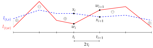
Figure 8: Signed area between two linear splines

Because the signed area function $S$ of (117) is simple, we are able to directly compute the corresponding proximity operators. In fact, the following result follows readily from Case 5 of Theorem 2.7:

Theorem 6.3 (proximity operators for $|S|$)

Let $l_{(t,x)}$ and $l_{(t,w})$ be two linear splines (see (3), and let $S$ be given by (117), i.e., the function corresponding to the signed area between the splines. Let $\gamma\in\mathbb{R}_{++}$ and let $\alpha\in\mathbb{R}_{++}$. Then

(118a) $$\operatorname{P}_{\gamma|\alpha S|}(x)=x-(\gamma\alpha)\operatorname{P}_{[-1,1]}\Big{(}\tfrac{\left\langle{\eta},{x-w}\right\rangle}{\gamma\alpha\|\eta\|^{2}}\Big{)}\eta$$

and

(118b) $$\operatorname{P}_{\gamma|\alpha S|^{*}}(x)=\alpha\operatorname{P}_{[-1,1]}\Big{(}\tfrac{\left\langle{\eta},{x-\gamma w}\right\rangle}{\alpha\|\eta\|^{2}}\Big{)}\eta.$$

6.3 Cost functions related to areas in road design problems

In road design problems, one assumes that the original (vertical) ground profile is represented by the linear spline $l_{(t,w)}$ (see [4] for details). It is required to find a vector $x\in C_{1}\cap\cdots C_{6}$ that is as “close” as possible to the vector $w$. There are several ways to measure this closeness; of particular interest are the following quantities:

• the amount of earth work (cut and fill) needed. This amount can be interpreted as the absolute area $A(x)$ between the two linear splines $l_{(t,x)}$ and $l_{(t,w)}$, which is given by (111) or its polyhedral approximations.

• the final cut-and-fill balance. In practice, the soil obtained from cutting can be used later for filling. Therefore, the engineer is also interested in minimizing the final cut-and-fill balance. This amount is interpreted as the absolute value of the signed area $S(x)$ (see (117)).

The measures may be combined by taking conical (i.e., positive linear) combinations. Thus, the problem of interest is to

(119) $${\rm Minimize}\quad\alpha A(x)+\beta|S|(x)\quad\text{subject to}\quad x\in C_{1}\cap\cdots\cap C_{6},$$

where $A(x)$ is given by (111), $S(x)$ is given by (117), and $\alpha$ and $\beta$ are nonnegative weights.

7 Douglas–Rachford and Cyclic Intrepid Projections algorithms

In this section we briefly review two algorithms we will employ in numerical experiments. Recall that $X=\mathbb{R}^{N}$ and let $I$ be a nonempty finite set of indices.

7.1 Douglas–Rachford Algorithm (DR)

Consider the problem

(120) $$\text{minimize}\quad\sum_{i\in I}f_{i}(x)\quad\text{subject to}\quad x\in X,$$

where each $f_{i}$ are proper convex lower semicontinuous function on $X$. The Douglas–Rachford algorithm, or simply “DR” solves (120) by operating in the product Hilbert space

(121) $$\mathbf{X}:=X^{I},$$

with inner product $\left\langle{\mathbf{x}},{\mathbf{y}}\right\rangle:=\sum_{i\in I}\left\langle{x_{i}},{y_{i}}\right\rangle$ for $\mathbf{x}=(x_{i})_{i\in I}$ and $\mathbf{y}=(y_{i})_{i\in I}$. Its precise formulation is as follows (see, e.g., [2, Proposition 27.8]):

Initialize $\mathbf{x}_{0}=(x_{0,i})_{i\in I}=(z,\ldots,z)\in\mathbf{X}$, where $z\in X$. Given $\mathbf{x}_{k}\in\mathbf{X}$, update via

(122a) $$\overline{x}_{k} :=\frac{1}{|I|}\sum_{i\in I}x_{k,i},$$

(122b) $$(\forall i\in I)\quad y_{k,i} :=\operatorname{P}_{\gamma f_{i}}(2x_{k,i}-\overline{x}_{k}),$$

(122c) $$(\forall i\in I)\quad x_{k+1,i} :=x_{k,i}+y_{k,i}-\overline{x}_{k},$$

to obtain $\mathbf{x}_{k+1}$. Then the monitored sequence $(\overline{x}_{k})_{{k\in{\mathbb{N}}}}$ converges to a solution of (120).

DR finds its roots in the field of differential equations [13]. The seminal work by Lions and Mercier [17] broad to light the much wider scope of this algorithm. Nowadays, there are several variants and numerous studies of DR. We do not describe these variants here because the two modern ones we experimented with (see [6] and [7]) performed similarly to the plain vanilla DR.

7.2 Method of Cyclic Intrepid Projections (CycIP)

To describe the method of cyclic intrepid projections, which has its roots in [15], we first need to develop the notion of an intrepid projector. Suppose that $Z$ is a nonempty closed convex subset of $X$ and let $\beta\in\mathbb{R}_{++}$. Set $C:=\big{\{}{x\in X}~{}\big{|}~{}{d_{Z}(x)\leq\beta}\big{\}}$. Then the corresponding intrepid projector onto $C$ (with respect to $Z$ and $\beta$) is defined by

(123) $$Q_{C}\colon X\to X\colon x\mapsto\begin{cases}P_{Z}x,&\text{if $d_{Z}(x)\geq 2\beta$;}\\ x,&\text{if $d_{Z}(x)\leq\beta$;}\\ x+\big{(}\beta-d_{Z}(x)\big{)}\displaystyle\frac{x-P_{Z}x}{\beta},&\text{otherwise.}\end{cases}$$

Consider the convex feasibility problem

(124) $$\text{find}\quad x\in C:=\bigcap_{i\in I}C_{i}\neq\varnothing,$$

where each $C_{i}$ is a nonempty closed convex subset of $X$. Define $I_{0}$ by $i\in I_{0}$ if and only if $i\in I$ and $T_{i}:=Q_{C_{i}}$ is an intrepid projector onto $C_{i}$; for $i\in I_{1}:=I\smallsetminus I_{0}$, we set $T_{i}:=P_{C_{i}}$. Given $x_{0}\in X$, the method of cyclic intrepid projections (CycIP) generates a sequence $(x_{k})_{k\in{\mathbb{N}}}$ in $X$ via

(125) $$(\forall{k\in{\mathbb{N}}})\quad x_{k+1}=\big{(}T_{m}T_{m-1}\cdots T_{2}T_{1}\big{)}x_{k}$$

Then the monitored sequence $(x_{k})_{k\in{\mathbb{N}}}$ converges to some point in $C$ (see [3, Theorem 14]).

CycIP is just one of many projection methods for solving (124) (see [1], [8], [9], [10] and the references therein); however, CycIP performed very well in the context of road design (see [3] and [4]).

8 Numerical experiments

We now return to the optimization problem (119). In the context of road design and construction, $\alpha$ is an averaged unit cost for excavation and embankment, and $\beta$ is an averaged unit cost for hauling. The values for $\alpha$ and $\beta$ change with soil types and vary by location; however, setting $\alpha:=4$ and $\beta:=1$ is a reasonable assignment based on actual handling cost.

We will consider Douglas–Rachford algorithm to solve (119) with three different estimates of $A(x)$:

• DRsb: solve problem (119) where $A(x)$ is the exact earth work amount, i.e., using the stadium norm.

• DRhb: solve problem (119) where $A(x)$ is the upper estimate of earth work amount using the hexagonal stadium norm.

• DRlb: solve problem (119) where $A(x)$ is the upper estimate of earth work amount using $\ell=\|\cdot\|_{1}$.

Note that at the very least, the engineer must solve the road design feasibility problem

(126) $${\rm find}\quad x\in C_{1}\cap\cdots\cap C_{6}.$$

Thus, it is important and interesting to see how much earthwork one can save by solving the optimization problem (119) rather than the mere feasibility problem (126). Indeed, solving (126) has been extensively studied in [4]. In particular, the experiments in [4] shows that the method of cyclic intrepid projections (CycIP) is an extremely fast and efficient algorithm for solving (126) (for further information on CycIP see [3]). Therefore, we will compare the cost-efficiency of DRsb, DRhb, and DRlb to CycIP.

8.1 Setup and stopping criteria

Because the Douglas–Rachford algorithm requires the proximity operators of all function involved, we write (119) as

(127) $${\rm minimize}\quad\alpha A_{\rm odd}(x)+\alpha A_{\rm even}(x)+\beta|S|(x)+\sum_{i=1}^{6}\iota_{C_{i}}(x)\quad\text{over}\quad x\in X$$

in order to use the explicit proximity formulas given in Theorems 2.7 and 5.4.

We run the four algorithms described above on $100$ test problems: 6 of which are obtained from real terrain data in British Columbia (Canada), and the rest of which is taken from the test problems in [4, Section 6]. We set our tolerance at

(128) $$\varepsilon:=5\cdot 10^{-3}.$$

Since CycIP is an algorithm aimed at solving the underlying feasibility problem, we stop it as soon as a term of the monitored sequence $(x_{k})_{k\in{\mathbb{N}}}$ satisfies

(129) $$\max_{i\in\{1,\ldots,6\}}\|x_{k}-P_{C_{i}}x_{k}\|_{\infty}<\varepsilon.$$

For DRsb, DRhb, DRlb, the Douglas–Rachford-based optimization algorithms, we terminate when the first term $\overline{x}_{k}$ of the monitored sequence $(\overline{x}_{k})_{k\in{\mathbb{N}}}$ satisfies

(130) $$\max_{i\in\{1,\ldots,6\}}\|\overline{x}_{k}-P_{C_{i}}\overline{x}_{k}\|_{\infty}<\varepsilon\quad\text{and}\quad\|\overline{x}_{k}-\overline{x}_{k-1}\|_{\infty}<\varepsilon.$$

8.2 Cost savings

Although DRsb, DRhb, and DRlb deal with different cost approximations, we are interested in comparing the exact earthwork cost: recall that given the ground profile $(t,w)$, the exact earthwork amount for a road design $(t,x)$ is

(131) $$F(x):=\alpha A(x)+\beta|S|(x),$$

where $A(x)$ is the exact area between two splines $l_{(t,x)}$ and $l_{(t,w)}$, and $S(x)$ is the signed area between these two splines (see Sections 6.1 and 6.2).

For each problem, let $F_{\rm CycIP}$ and $F_{\rm DR}$ be the cost of the road designs obtained by CycIP and DR, respectively. Then the cost saving ratio is given by

(132) $$\Delta_{\rm DR}:=\frac{F_{\rm CycIP}-F_{\rm DR}}{F_{\rm CycIP}}.$$

In the following table, we record the statistics for $\Delta_{\rm DRsb}$, $\Delta_{\rm DRhb}$, and $\Delta_{\rm DRlb}$.

	Min	1st Qrt.	Median	3rd Qrt.	Max	Mean	Std.dev.
$\Delta_{\rm DRsb}$	$-0.11\%$	6.38%	12.4%	18.82%	73.58%	14.90%	13.91%
$\Delta_{\rm DRhb}$	$-0.49\%$	6.02%	11.96%	18.46%	72.23%	14.56%	13.75%
$\Delta_{\rm DRlb}$	$-0.12\%$	5.30%	11.41%	17.00%	72.73%	13.87%	13.19%

Table 1: Cost savings: DR vs. CycIP (higher is better)

Theoretically, we expect the cost saving of every optimization algorithm to be nonnegative. However, we observe (small) negative savings by either DR algorithms in $8$ out of $100$ test problems. In fact, because of the $\varepsilon$-tolerance in our stopping criteria, the DR algorithms might stop before attaining optimality.

8.3 Performance profiles

To compare the performance of the algorithms, we use performance profiles: for every $a\in\mathcal{A}$ and for every $p\in\mathcal{P}$, we set

(133) $$r_{a,p}:=\frac{k_{a,p}}{\min\big{\{}{k_{a^{\prime},p}}~{}\big{|}~{}{a^{\prime}\in\mathcal{A}}\big{\}}}\geq 1,$$

where $k_{a,p}\in\{1,2,\ldots,k_{\max}\}$ is the number of iterations that $a$ requires to solve $p$ and $k_{\max}$ is the maximum number of iterations allowed for all algorithms. If $r_{a,p}=1$, then $a$ uses the least number of iterations to solve problem $p$. If $r_{a,p}>1$, then $a$ requires $r_{a,p}$ times more iterations for $p$ than the algorithm that uses the least number of iterations for $p$. For each algorithm $a\in\mathcal{A}$, we plot the function

(134) $$\rho_{a}\colon\mathbb{R}_{+}\to[0,1]\colon\kappa\mapsto\frac{\operatorname{card}\big{\{}{p\in\mathcal{P}}~{}\big{|}~{}{\log_{2}(r_{a,p})\leq\kappa}\big{\}}}{\operatorname{card}\mathcal{P}},$$

where “$\operatorname{card}$” denotes the cardinality of a set. Thus, $\rho_{a}(\kappa)$ is the percentage of problems that algorithm $a$ solves within factor $2^{\kappa}$ of the best algorithms. Therefore, an algorithm $a\in\mathcal{A}$ is “fast” if $\rho_{a}(\kappa)$ is large for $\kappa$ small; and $a$ is “robust” if $\rho_{a}(\kappa)$ is large for $\kappa$ large.

The following figure shows the performance profiles for the three DR algorithms.

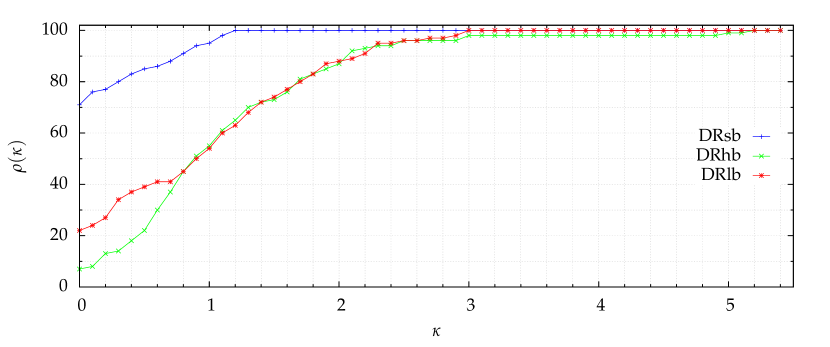
Figure 9: Performance profiles (by number of iterations)

Note that, the performance profiles only reflect the number of iterations needed, but they do not take into account the complexity of proximity operator computations.

8.4 Problems with real terrain data of BC

In this section, we present the statistics for the 6 problems that use real terrain data of British Columbia (Canada). The problems represent 6 different design alternatives for a (hypothetical) high-speed bypass of the city of Merritt, which would connect Highway 97C directly with the Coquihalla Highway. The bypass starts at the intersection of the Okanagan Connector Hwy 97C with the Princeton-Kamloops Hwy 5A, and follows westwards, joining the Coquihalla Hwy 5 near the Kane Valley and Coldwater Rd intersection.

As an example, one of the problems is to build a highway alternative that is $27.805$ kilometer long and $10.4$ meter wide with a design speed of $110$ km/h and a maximum slope of $5\%$. Starting from the original ground profile (the brown curve in Figure 10), we select the points $(t_{i},w_{i})_{i\in\{1,\ldots,n\}}$ and create the initial road design $l_{(t,w)}$ (which is the linear spline generated by the chosen points).

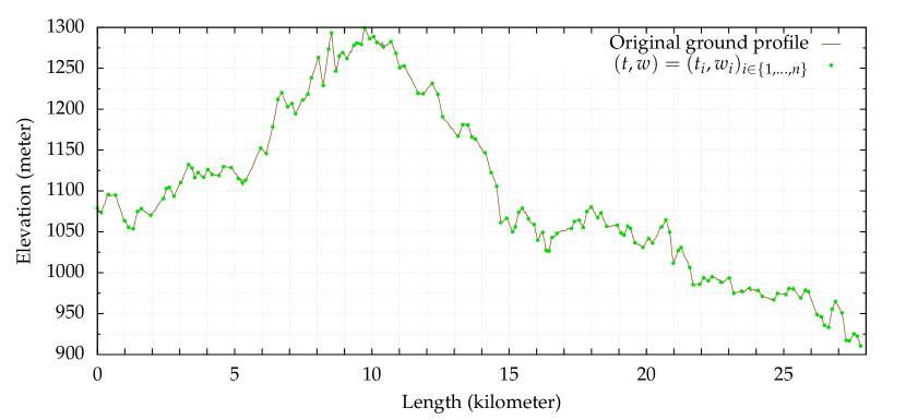
Figure 10: Initial road design $l_{(t,w)}$ from the original ground profile.

This initial design $l_{(t,w)}$ is usually infeasible, and we use $w$ as the starting point for the algorithms. The following two figures show the so-obtained road designs.

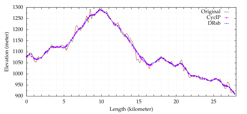
Figure 11: Road designs obtained by CycIP and DRsb.

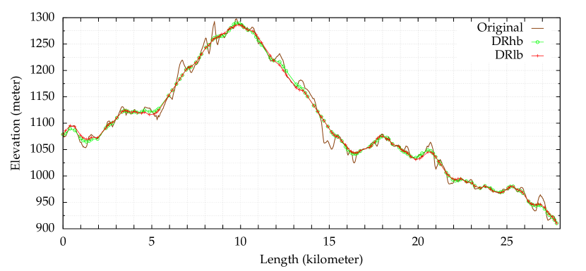
Figure 12: Road designs obtained by DRhb and DRlb.

These road designs are indeed different as seen in the two diagrams below. Figure 13 presents a mass diagram. The mass diagram is a plot of the cut and fill volumes along the road (where cuts are positive and fills are negative). Hence, a mass diagram that finishes closer to zero indicates a better balance between cut and fill. Figure 14 shows a cumulative mass diagram, where cut and fills are both taken as positive.

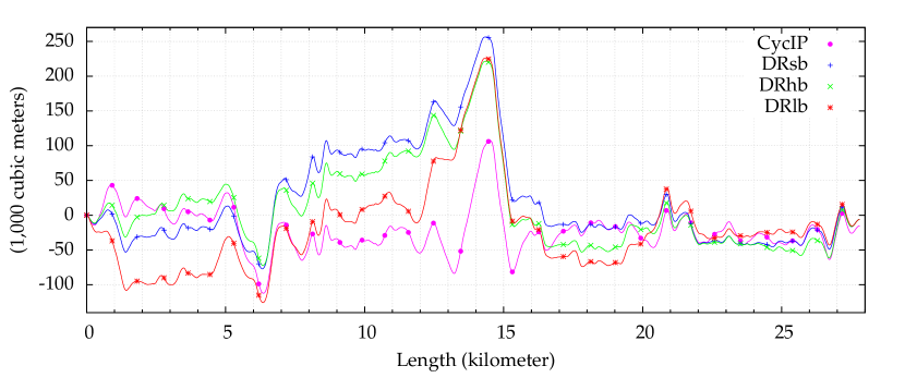
Figure 13: Mass diagrams

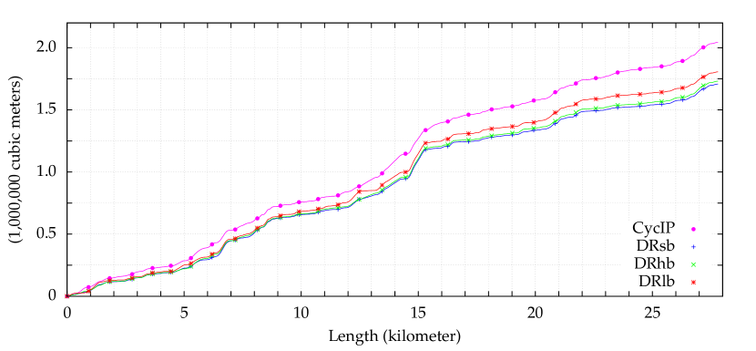
Figure 14: Cumulative cut-and-fill amount

We set the cost for cut-and-fill at $5.23 per cubic meter and the cost for handling the final cut-and-fill balance at $1.31 per cubic meter (notice that the ratio of these two costs is approximately $4\negthinspace:\negthinspace 1$). From the obtained data we then record the cost for each road design in the next table.

Algorithms	Cut-and-fill (${\rm m}^{3}$)	Final balance (${\rm m}^{3}$)	Earthwork cost ($)	Saving (%)
CycIP	$2,043,188.4$	$-15,273.0$	$10,703,303$	$0\%$
DRsb	$1,707,709.5$	$-5,960.7$	$8,936,992$	$16.50\%$
DRhb	$1,730,857.5$	$-5,996.8$	$9,058,059$	$15.37\%$
DRlb	$1,805,893.0$	$-6,036.3$	$9,450,468$	$11.71\%$

Table 2: Earthwork amount and cost saving

8.5 Conclusion

The results suggest the following:

• Employing the cost function may reduce the construction cost significantly. In our particular problem, DRsb can save approximately $1.76$ million dollars ($16.5\%$), while the savings of DRhb and DRlb are $1.64$ and $1.25$ millions ($15.37\%$ and $11.71\%$), respectively.

• Using the exact cost function (i.e., DRsb) may lead to a greater saving.

• Using the hexagonal approximation (i.e., DRhb) is beneficial for programming purpose while also maintaining a good saving percentage.

The data for the other 5 problems listed next also support our observations.

Algorithms	Prob. 1	Prob. 2	Prob. 3	Prob. 4	Prob. 5
DRsb	$7.05\%$	$10.35\%$	$8.88\%$	$18.96\%$	$12.81\%$
DRhb	$7.00\%$	$10.41\%$	$8.49\%$	$18.17\%$	$12.45\%$
DRlb	$6.88\%$	$6.35\%$	$7.7\%$	$16.0\%$	$10.04\%$

Table 3: Cost savings over CycIP

In summary, the experiments support our belief that the road design optimization problem can be efficiently solved by employing variants of the Douglas–Rachford algorithm. Future work may concentrate on refining the model and on testing the algorithms on large-scale data using graphics processing units.

References

- [1] H.H. Bauschke and J.M. Borwein, On projection algorithms for solving convex feasibility problems, SIAM Review 38 (1996), pp. 367–426.
- [2] H.H. Bauschke and P.L. Combettes, Convex Analysis and Monotone Operator Theory in Hilbert Spaces, Springer, 2011.
- [3] H.H. Bauschke, F. Iorio, and V.R. Koch, The method of cyclic intrepid projections: convergence analysis and numerical experiments, in The Impact of Applications on Mathematics, Proceedings of the Forum of Mathematics for Industry (Fukuoka 2013), M. Wakayama et al. (editors), Springer 2014, pp. 187–200.
- [4] H.H. Bauschke and V.R. Koch, Projection methods: Swiss Army knives for solving feasibility and best approximation problems with halfspaces, in Proceedings of the workshop on Infinite Products of Operators and Their Applications (Haifa 2012), S. Reich and A. Zaslavski (editors), Contemporary Mathematics, in-press.
- [5] H.H. Bauschke, Y. Lucet, and H.M. Phan, On the convexity of piecewise-defined functions, preprint, http://arxiv.org/abs/1408.3771, August 2014.
- [6] R.I. Boţ, E.R. Csetnek, and A. Heinrich, A primal-dual splitting algorithm for finding zeros of sums of maximally monotone operators, SIAM Journal on Optimization 23 (2013), pp. 2011–2036.
- [7] L.M. Briceño-Arias and P.L. Combettes, A monotone+skew splitting model for composite monotone inclusions in duality, SIAM Journal on Optimization 21 (2011), pp. 1230–1250.
- [8] A. Cegielski, Iterative Methods for Fixed Point Problems in Hilbert Spaces, Springer 2012.
- [9] Y. Censor and S.A. Zenios, Parallel Optimization, Oxford University Press, 1997.
- [10] P.L. Combettes, Hilbertian convex feasibility problems: convergence of projection methods, Applied Mathematics and Optimization 35 (1997), pp. 311–330.
- [11] P.L. Combettes and J.-C. Pesquet, Proximal splitting methods in signal processing, in Fixed-Point Algorithms for Inverse Problems in Science and Engineering, H.H. Bauschke et al. (editors), Springer, 2011, pp 185–212.
- [12] E.D. Dolan and J.J. Moré, Benchmarking optimization software with performance profiles, Mathematical Programming (Series A) 91 (2002), pp. 201–213.
- [13] J. Douglas and H.H. Rachford, On the numerical solution of heat conduction problems in two and three space variables, Transactions of the AMS 82 (1956), pp. 421–439.
- [14] Gnuplot, http://sourceforge.net/projects/gnuplot
- [15] G.T. Herman, A relaxation method for reconstructing objects from noisy x-rays, Mathematical Programming 8 (1975), pp. 1–19.
- [16] The Julia Language, http://julialang.org
- [17] P.-L. Lions and B. Mercier, Splitting algorithms for the sum of two nonlinear operators, SIAM Journal on Numerical Analysis 16 (1979), pp. 964–970.
- [18] J.-J. Moreau, Proximité et dualité dans un espace hilbertien, Bulletin de la Société Mathématique de France 93 (1965), pp. 273–299.
- [19] R.T. Rockafellar. Convex Analysis. Princeton University Press, 1970.