Scales of a fluid

Abstract

The flow of a viscous fluid is perturbed by its internal friction which generates heat and leads to a small temperature change. This does not occur for an ideal fluid. We would like to resolve this picture as a function of the dynamical macroscopic scales of both problems. In order to do this we will study the evolution of the Navier-Stokes Hamiltonian with the classical similarity renormalization group in the region of small viscosity. The connection between the Euler and Navier-Stokes fluids will be pursued, but also the viscous structures that arise will be studied in their own right to determine the low-order velocity correlators of realistic fluids such as single-component air and water. The canonical coordinate of the Navier-Stokes Hamiltonian is a vector field that stores the initial position of all the fluid particles. Thus these appear to be natural coordinates for studying arbitrary separations of fluid particles over time. This connection will be pursued and the region where the classic 1926 Richardson 4/3 scaling law holds will be determined. The evolution of the Euler Hamiltonian will also be studied and we will attempt to map its singular structures to those of the small-viscosity Navier-Stokes fluid.

I Introduction

The Navier-Stokes and Euler equations of fluid dynamics apparently do not map smoothly onto each other in the limit of vanishing viscosity: the zero viscosity and infinitesimal viscosity fluids do not appear to be limits of the same theory. Singular velocity gradients are the culprit, but we would like to understand this connection better. We therefore focus on the energy dissipation aspect of the Navier-Stokes equation in local thermodynamic equilibrium. The dissipation term of the heat equation due to the internal friction (viscosity) of a fluid is just another volume heat source that increases the temperature of the fluid slightly, however it is still a closed thermodynamic system and can be studied with Hamiltonian techniques. Thus, the Navier-Stokes Hamiltonian is derived from first principles including the nonholonomic entropy constraint and it is shown that the dynamical coordinate of a dissipative fluid is a vector field that stores the initial position of all the fluid particles—these appear to be natural coordinates for studying arbitrary separations of fluid particles over time.

The Euler and Navier-Stokes Hamiltonians are used to compare the vanishing viscosity limit between the two theories. It is shown that they have the same number of degrees of freedom in three spatial dimensions: six independent scalar potentials; but in the Navier-Stokes case, the potentials are actually two vector fields that are canonical coordinate-momentum field pairs. Thus, in these “coordinates” it is easy to see that the two theories have different dynamical degrees of freedom (fields). We will study this connection further to understand its dynamical consequences better. A final motivation for using Hamiltonian field theory techniques is that they allow convenient approximations and can be used to systematically integrate the equations of motion of a fluid one scale at a time with the similarity renormalization group which has been shown to be fruitful in nuclear and condensed matter physics. The connection to classical physics follows from the canonical Poisson bracket structure of the fields of the Navier-Stokes Hamiltonian along with its Poisson bracket with an arbitrary classical dissipative observable. Thus the stage has been set to study the scales of a classical fluid (see Fig. 1) and to better understand the connection between the Euler and Navier-Stokes theories in the limit of vanishing but nonzero viscosity—heat and eventually diffusion will matter in this work.

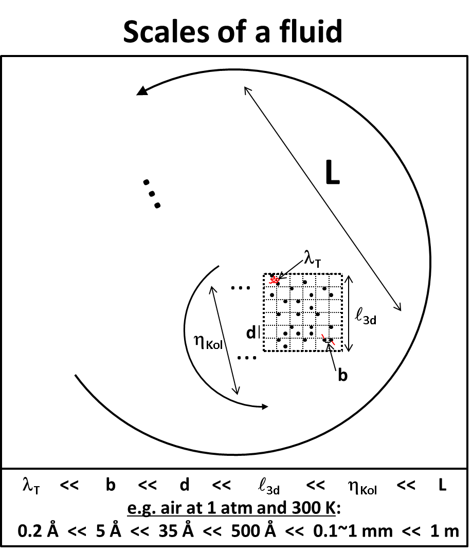
Figure 1: A typical fluid eddy of size $L$ with its macroscopic and microscopic substructure. A Kolmogorov microscale eddy of size $\eta_{Kol}$ is the smallest macroscopic structure. The successive microscopic substructure is the mean free path $\ell_{3d}$, the average molecular separation $d$, the molecular impact parameter $b$ and the thermal wavelength $\lambda_{T}$. For air at room temperature, all of these scales are separated by at least an order of magnitude as shown. For water, the story is similar but then $b$, $d$, and $\ell_{3d}$ are all of the same order of magnitude with the microscopic degrees of freedom strongly coupled. Nevertheless in both cases (air and water) $\lambda_{T}$ is much smaller than the average separation between the molecules themselves and their quantum nature is therefore inaccessible. In addition, in both cases, the mean free path is much smaller than dissipation scale $\eta_{Kol}$ and macroscale $L$; therefore the continuum approximation is valid and the Navier-Stokes equation becomes the paradigm of interest.

II Dynamics of a fluid

The dynamics of a nonrelativistic classical single-component fluid are given by the equations of motion for its velocity, density and entropy fields landau :

$$\rho D_{t}v_{i}=-\partial_{i}p+\partial_{j}\sigma^{\prime}_{ij}\;,~{}~{}D_{t}\rho=-\rho\mathbf{\nabla}\cdot\mathbf{v}\;,~{}~{}\rho TD_{t}s=\sigma^{\prime}_{ij}\partial_{j}v_{i}-\mathbf{\nabla}\cdot\mathbf{q}\;,$$

where $D_{t}=\partial_{t}+\mathbf{v}\cdot\mathbf{\nabla}$ is the convective derivative with $\partial_{t}$ being a shorthand for $\frac{\partial}{\partial t}$. Repeated indices are summed over the three spatial dimensions and $\partial_{i}$ is a shorthand for $\frac{\partial}{\partial x_{i}}$. $p$ is pressure, $T$ is temperature, $\sigma^{\prime}_{ij}$ is the viscous stress tensor and $\mathbf{q}$ is the heat flux defined as $\mathbf{q}=-\kappa\,\mathbf{\nabla}T$ where $\kappa$ is the thermal conductivity. The viscous stress tensor for a Newtonian fluid (which defines the Navier-Stokes equation—the first relation above for $D_{t}v_{i}$) is given by

$$\sigma^{\prime}_{ij}\equiv\eta(\partial_{i}v_{j}+\partial_{j}v_{i})+\zeta^{\prime}\delta_{ij}\mathbf{\nabla}\cdot\mathbf{v}\;,$$

where $\eta$ and $\zeta$ are the shear and bulk viscosity respectively and $\zeta^{\prime}\equiv\zeta-2\eta/3$—defined such that the trace of the viscous stress tensor is independent of shear viscosity.

We carefully wrote these complete equations of motion to be concrete: this is what we mean by the “Navier-Stokes paradigm” mentioned in Fig. 1. The Navier-Stokes Hamiltonian written below reproduces these equations of motion exactly as shown in Hns ; Hiroki . The entropy equation of motion above is known as the heat equation and is a nonholonomic (path-dependent) constraint Goldstein on the motion of the fluid. Note how the viscous stress tensor, $\sigma^{\prime}_{ij}$, is in both the heat equation and the Navier-Stokes equation itself: this is how the heat generated by the internal friction of the fluid gets coupled into its motion and causes the temperature to rise in its own wake so to say. It is a self-energy correction for the system, but energy is still conserved since “heat” is included in what we mean by energy (the main lesson of thermodynamics).

These equations of motion follow from first principles of momentum, mass and energy conservation landau . As shown in Hns ; Hiroki , they also follow from the Euler-Lagrange equations of their respective Lagrangian, and the Hamilton equations of their respective Hamiltonian. We use the Lagrangian to derive the initial Hamiltonian (which gets changed due to renormalization) but in what follows to keep the discussion clearer, hereafter we only discuss Hamiltonians. The interesting thing is that starting from first principles one is led to a drastically different form Hns for the Hamiltonian of the Euler and Navier-Stokes fluids (defined as fluids satisfying the respective equation). Note that the equations of motion for the Euler fluid are the same as the above with $\sigma^{\prime}_{ij}$ set to zero (which includes removing gradients! and is not just setting viscosity to zero).

Here we write the kinematic results for the difference between the Navier-Stokes and Euler Hamiltonian degrees of freedom. For this work, we would like to pursue the dynamical consequences of this difference using the similarity renormalization group (described in the next section) to evolve the Navier-Stokes Hamiltonian from its macroscopic small to large scales ($\eta_{Kol}$ through $L$—see Fig. 1) to obtain the velocity correlation functions and particle separation distributions of the theory at scale ‘s’ and time ‘t’.

For the ideal fluid, the Euler Hamiltonian density is given by Hns ; Hiroki ; Zakharov

$${\cal H}_{E}(\rho,\phi;\beta,\alpha;s,\lambda)=\frac{1}{2}\rho\left(\mathbf{\nabla}\phi-\frac{\alpha}{\rho}\mathbf{\nabla}\beta-\frac{\lambda}{\rho}\mathbf{\nabla}s\right)^{2}+{\cal U}(\rho,s)\;.$$

Note that the arguments of ${\cal H}_{E}$ on the left are written in terms of its three dynamical coordinate fields: $\rho$, $\beta$, and $s$; and their respective conjugate momentum fields: $\phi$, $\alpha$, and $\lambda$. $\rho$ and $s$ are the same density and entropy field as in the equations of motion above. $\phi$ is the same velocity potential as in potential flow fluid mechanics ($\mathbf{v}=\mathbf{\nabla}\phi$). $\alpha$ and $\beta$ are a Clebsch-potential pair and $\lambda$ is the lagrange multiplier field for the entropy constraint of an ideal fluid (i.e. $D_{t}s=0$). ${\cal U}$ is the internal energy density. Again, see Hns for further details, but note that a Hamiltonian and its density are related by $H=\int d^{3}x\,{\cal H}$.

For the viscous fluid we are led to a very different Hamiltonian due to the dissipation term of the heat equation: $\sigma^{\prime}_{ij}\partial_{j}v_{i}\equiv\rho\,\varepsilon$, where $\varepsilon$ is the well-known energy dissipation field which in a region of fully-developed turbulent scaling is constant or nearly constant. This dissipation makes the entropy constraint nonholonomic and necessitates the introduction of vector field $\mathbf{X}(\mathbf{x},t)$ Hiroki in a fashion at least reminiscent of gauge invariance Zakharov . This new field $\mathbf{X}(\mathbf{x},t)$ is just a coordinate transformation, and as shown in Hiroki ; Hns it is a canonical transformation with the $(\mathbf{x},\mathbf{p})$ and $(\mathbf{X},\mathbf{P})$ pairs having the same Poisson bracket structure Goldstein . With all the algebra worked out in Hns , the Hamilton equations of the following Hamiltonian are equivalent to the equations of motion that led off this section. The Navier-Stokes Hamiltonian density is given by Hiroki

$${\cal H}_{NS}\left(\mathbf{X},\mathbf{P},s(\mathbf{X})\right)=\frac{(P_{i}\mathbf{\nabla}X_{i})^{2}}{2\,J(\mathbf{\nabla}\mathbf{X})\,\rho_{0}(\mathbf{X})}+{\cal U}(J(\mathbf{\nabla}\mathbf{X})\,\rho_{0}(\mathbf{X}),s(\mathbf{X}))\;.$$

The degrees of freedom of this Hamiltonian are coordinate vector field $\mathbf{X}(\mathbf{x},t)$ and its conjugate momentum vector field $\mathbf{P}(\mathbf{x},t)$. $s(\mathbf{X})$ is the same entropy field as in the heat equation, but here it is given by the following nonholonomic field variation constraint Hiroki ; Hns :

$$\frac{\delta s}{\delta X_{i}}=\left(\partial_{j}s+\frac{\partial_{k}\sigma_{jk}^{\prime}}{\rho\,T}\right)\frac{\partial x_{j}}{\partial X_{i}}\;.$$

Note that ${\cal H}_{NS}$ starts out quartic in the fields in the numerator of the first term and there is no standard quadratic term of field theory Lvov . $J(\mathbf{\nabla}\mathbf{X})$ is the Jacobian explicitly given in Hns with six terms in total and each term being cubic in $\partial_{j}X_{i}$, and for this first “$p^{2}/(2m)$” term it is in the denominator which makes its contributions nonlocal. Finally, $\rho_{0}(\mathbf{X})$ is the initial density set by the physics of the problem which often allows $\rho=J\rho_{0}$ to be approximated as a constant or near-constant mean and then to perturb about this mean. We would like to explore these ideas further with this work.

In summary, the Euler and Navier-Stokes fluids have quite different pathlines for their fluid particles given by their respective velocity field:

$$\mathbf{v}_{E} = \framebox{$\mathbf{\nabla}\phi-\frac{\alpha}{\rho}\mathbf{\nabla}\beta-\frac{\lambda}{\rho}\mathbf{\nabla}s$}\;,$$

$$\mathbf{v}_{NS} = \framebox{$-\frac{P_{i}}{\rho}\mathbf{\nabla}X_{i}$}=-\frac{P_{i}\mathbf{\nabla}X_{i}}{J(\mathbf{\nabla}\mathbf{X})\,\rho_{0}(\mathbf{X})}\;.$$

Vector field $\mathbf{X}$ is just another coordinate like $\mathbf{x}$, so the fact that there are three scalar potential pairs in the Navier-Stokes fluid $(X_{1},P_{1};X_{2},P_{2};X_{3},P_{3})$ is directly related to the choice of working in three spatial dimensions. The Navier-Stokes fluid seems to be perfectly coupled to three spatial dimensions. There are two further points to be made both highlighting the differences between the Euler and Navier-Stokes fluids even though upon first sight, these $\mathbf{v}_{E}$ and $\mathbf{v}_{NS}$ decompositions look similar. First, for $\mathbf{v}_{E}$ note how the $\mathbf{\nabla}\phi$ term has a plus sign and does not have any density dependence whereas the other two terms have opposite sign and have density dependence. For the Navier-Stokes fluid, the signs of all three terms can be made to be the same in $\mathbf{v}_{NS}$ with the conjugate momenta of ${\cal H}_{NS}$ related by a positive sign: $\pi_{X_{i}}=+P_{i}$, and there is no asymmetry in the density dependence. $\phi$ is of course the standard velocity potential of fluid mechanics and $\mathbf{v}_{E}$ is the so-called Clebsch decomposition of the velocity field with Gauss potential jackiw pairs ($\alpha$,$\beta$) and ($\lambda$,$s$). Interestingly, to obtain the Navier-Stokes Hamiltonian one had to introduce coordinate transformation $\mathbf{X}(\mathbf{x},t)$ in order to handle the entropy constraint properly and this already gave enough degrees of freedom and so a velocity potential was not required. The Euler and Navier-Stokes fluids are very different. Second, $\mathbf{v}_{E}$ and $\mathbf{v}_{NS}$ being different is even more readily apparent if we recall that $\rho$ is a dynamical field for the Euler fluid (satisfying the standard continuity equation), whereas for the Navier-Stokes fluid, $\rho=J\rho_{0}$ is a constraint which in terms of vector field $\mathbf{X}$ is quite complex: see Hns for an explicit expression for $J(\mathbf{\nabla}\mathbf{X})$. Also note that since $J$ (with derivatives of fields) is in the denominator, it is a nonlocal operator in ${\cal H}_{NS}$. These differences should not come as a huge surprise since the Euler and Navier-Stokes fluids apparently do not map smoothly onto each other: the zero viscosity and infinitesimal viscosity fluids do not appear to be limits of the same theory. Perhaps these variational principle forms of the theories help to make this clearer, and with this work we would like to pursue the dynamical consequences of this further.

The Poisson bracket structure of the fields of ${\cal H}_{NS}$ along with its Poisson bracket with an arbitrary dissipative observable is derived in Hns . This sets the stage for the similarity renormalization group (SRG) introduced in the next section. The connection between nuclear physics (the original arena of the SRG SRG ) and fluid dynamics is made through the Poisson bracket structure of the classical Hamiltonian of interest, in this case ${\cal H}_{NS}$.

III Classical similarity renormalization group

In order to better understand the scales of a classical fluid and the connection between the Euler and Navier-Stokes fluids we propose studying the physics of a viscous fluid as the viscosity vanishes. As is well known, on dimensional grounds $\eta_{Kol}\sim\nu^{3/4}/\varepsilon^{1/4}$, therefore this entails understanding the physics of a viscous fluid at it smallest macroscopic scales. We propose using the similarity renormalization group (SRG) to study the flow of the Navier-Stokes Hamiltonian from the smallest macroscopic scales, around $\eta_{Kol}$, (see Fig. 1) where the energy is dissipated through the largest scales, around $L$, where the energy is input.

The classical SRG acting on a Hamiltonian at scale $s$ (which can be thought of as the spatial “$s$ for size” of the region under study) is given by the following flow equation

$$\frac{dH_{s}}{ds}=-\left[\eta_{s},H_{s}\right]_{P.B.}\;,~{}~{}H_{s}\equiv H_{0}+V_{s}\;,~{}~{}\eta_{s}=[H_{0},V_{s}]_{P.B.}\;,$$

where ‘P.B’ implies ‘Poisson bracket’ and $\eta_{s}$ is the generator of this scale transformation. This is a new result based on the correspondence principle Sakurai applied to Wegner’s flow equation Wegner . Since it is a new result, we would like to show that the sign of this equation (which came from $i^{2}=-1$) is correct by comparing a simple fixed-source calculation in quantum field theory fixedsource with an analogous classical Hamiltonian: a harmonic oscillator with a linear potential due to, for example, gravity. Thus, say the starting classical Hamiltonian with coordinate $q$ and momentum $p$ is given by

$$H=\frac{p^{2}}{2}+\frac{q^{2}}{2}+g\,q\;,$$

with coupling $g$ (here the acceleration of gravity with unit mass and spring constant). In order to integrate out the effects of gravity (e.g. with the viscous fluid problem we could choose the dissipation operator of the entropy constraint here), next we choose

$$V=g\,q\;,$$

which implies that the free Hamiltonian is $H_{0}=\frac{p^{2}}{2}+\frac{q^{2}}{2}$. Sticking this $H_{0}$ and $V$ into the above classical SRG flow equation gives (hereafter we drop the designator “P.B”, but it is implied in all this work)

$$[H_{0},V] = \left[\frac{p^{2}}{2}+\frac{q^{2}}{2},g\,q\right]=-g\,p\;,$$

$$\frac{dH}{ds} = -\left[-g\,p\,,\,\frac{p^{2}}{2}+\frac{q^{2}}{2}+g\,q\right]=-g\,q-g^{2}\;,$$

using the standard rules of a Poisson bracket Goldstein . This last line is the result that corresponds exactly with like terms in the fixed-source quantum field theory problem fixedsource . Like there, in order to have a Hamiltonian with fixed structure as it runs with scale $s$, we change the initial Hamiltonian to the following ansatz, with a new “self-energy” term and a running coupling $g_{s}$:

$$H_{s}=\Sigma_{s}+\frac{p^{2}}{2}+\frac{q^{2}}{2}+g_{s}\,q\;.$$

Requiring consistency with this above $dH/ds$ result gives the following running coupling equations

$$\frac{dg_{s}}{ds}=-g_{s}\;,~{}~{}\frac{d\Sigma_{s}}{ds}=-g_{s}^{2}\;,$$

with solution

$$g_{s}=g_{0}\,e^{-s}\;,~{}~{}\Sigma_{s}=\Sigma_{s0}-\frac{g_{0}^{2}}{2}\left[e^{-2s_{0}}-e^{-2s}\right]\;.$$

The initial scale is $s=0$ and as $s\rightarrow\infty$ we see the gravity interaction is integrated out, with the self-energy $\Sigma_{s}$ dressed with a background field like in the Yukawa meson-cloud problem fixedsource , but here derived completely in the context of classical physics. The parallelism between the analogy is quite striking showing the correct sign identification for the above classical SRG flow equation.

IV Summary

The prime directive of this work is to understand the renormalization of the Navier-Stokes Hamiltonian through the classical similarity renormalization group to help elucidate the connection between the ideal and viscous theories. We will seek the connection first from studying the small-scale macroscopic structures of the viscous theory near the Kolmogorov scale as the dissipation operator is run with similarity scale $s$. Since the Navier-Stokes Hamiltonian dynamical coordinate is a vector field that stores the initial positions of all the fluid particles, we propose the study of its low-order velocity correlators and particle separation distributions as a function of scale, in order to determine the region for which the classic Richardson 4/3 scaling law holds turbvoyage . If the correct scales are resolved, the mechanism for the internal friction giving rise to heat and motion should be more readily apparent. The classical similarity renormalization group flow equation and Navier-Stokes Hamiltonian could shed new light on an old problem.

References

- (1) L. D. Landau and E. M. Lifshitz, Fluid Mechanics (Pergamon Press, 1989).
- (2) H. Fukagawa and Y. Fujitani, Prog. Theor. Phys. 124, 517 (2010); 127, 921 (2012); H. Fukagawa, Improvements in the Variational Principle for Fluid Dynamics (Diss. Keio Univ., 2012).
- (3) B. D. Jones, Navier-Stokes Hamiltonian (arXiv:1407.1035 [physics.flu-dyn], 2014).
- (4) H. Goldstein, Classical Mechanics (Addison-Wesley, 1980).
- (5) V. E. Zakharov and E. A. Kuznetsov, Hamiltonian formalism for nonlinear waves, Physics-Uspekhi 40, 1087 (1997).
- (6) V. S. L’vov, Physics Reports 207, 1–47 (1991).
- (7) R. Jackiw and A. P. Polychronakos, Phys. Rev. D 62, 085019 (2000), footnote 1.
- (8) St. D. Głazek and K. G. Wilson, Phys. Rev. D 48, 5863 (1993); 49, 4214 (1994); 57, 3558 (1998).
- (9) J. J. Sakurai, Modern Quantum Mechanics (Addison-Wesley, 1994).
- (10) F. Wegner, Ann. Phys. (Leipzig) 3, 77 (1994); F. J. Wegner, Physics Reports 348, 77 (2001).
- (11) B. D. Jones and R. J. Perry, Similarity flow of a neutral scalar coupled to a fixed source (arXiv:1305.6599 [hep-ph], 2013).
- (12) P. A. Davidson et al., A Voyage Through Turbulence (Cambridge, 2011), p. 190ff.