The Odds of Staying on Budget

Abstract

Given Markov chains and Markov decision processes (MDPs) whose transitions are labelled with non-negative integer costs, we study the computational complexity of deciding whether the probability of paths whose accumulated cost satisfies a Boolean combination of inequalities exceeds a given threshold. For acyclic Markov chains, we show that this problem is PP-complete, whereas it is hard for the PosSLP problem and in PSpace for general Markov chains. Moreover, for acyclic and general MDPs, we prove PSpace- and EXP-completeness, respectively. Our results have direct implications on the complexity of computing reward quantiles in succinctly represented stochastic systems.

1 Introduction

Computing the shortest path from $s$ to $t$ in a directed graph is a ubiquitous problem in computer science, so shortest-path algorithms such as Dijkstra’s algorithm are a staple for every computer scientist. These algorithms work in polynomial time even if the edges are weighted, so questions of the following kind are easy to answer:

(I) Is it possible to travel from Copenhagen to Kyoto in less than 15 hours?

From a complexity-theoretic point of view, even computing the length of the shortest path lies in NC, the class of problems with “efficiently parallelisable” algorithms.

The shortest-path problem becomes more intricate as soon as uncertainties are taken into account. For example, additional information such as “there might be congestion in Singapore, so the Singapore route will, with probability 10%, trigger a delay of 1 hour” naturally leads to questions of the following kind:

(II) Is there a travel plan avoiding trips longer than 15 hours with probability $\geq 0.9$?

Markov decision processes (MDPs) are the established model to formalise problems such as (II). In each state of an MDP some actions are enabled, each of which is associated with a probability distribution over outgoing transitions. Each transition, in turn, determines the successor state and is equipped with a non-negative “weight”. The weight could be interpreted as time, distance, reward, or—as in this paper—as cost. For another example, imagine the plan of a research project whose workflow can be modelled by a directed weighted graph. In each project state the investigators can hire a programmer, travel to collaborators, acquire new equipment, etc., but each action costs money, and the result (i.e., the next project state) is probabilistic. The objective is to meet the goals of the project before exceeding its budget for the total accumulated cost. This leads to questions such as:

(III) Is there a strategy to stay on budget with probability $\geq 0.85$?

MDP problems like (II) and (III) become even more challenging when each transition is equipped with both a cost and a utility, e.g. in order to model problems that aim at maximising the probability that both a given budget is kept and a minimum total utility is achieved. Such cost-utility trade-offs have recently been studied in [3].

The problems (II) and (III) may become easier if there is no non-determinism, i.e., there are no actions. We then obtain Markov chains where the next state and the incurred transition cost are chosen in a purely probabilistic fashion. Referring to the project example above, the activities may be completely planned out, but their effects (i.e. cost and next state) may still be probabilistic, yielding problems of the kind:

(IV) Will the budget be kept with probability $\geq 0.85$?

Closely related to the aforementioned decision problems is the following optimisation problem, referred to as the quantile query in [2, 3, 23]. A quantile query asked by a funding body, for instance, could be the following:

(V) Given a probability threshold $\tau$, compute the smallest budget that suffices with probability at least $\tau$.

Non-stochastic problems like (I) are well understood. The purpose of this paper is to investigate the complexity of MDP problems such as (II) and (III), of Markov-chain problems such as (IV), and of quantile queries like (V). More formally, the models we consider are Markov chains and MDPs with non-negative integer costs, and the main focus of this paper is on the cost problem for those models: Given a budget constraint $\varphi$ represented as a Boolean combination of linear inequalities and a probability threshold $\tau$, we study the complexity of determining whether the probability of paths reaching a designated target state with cost consistent with $\varphi$ is at least $\tau$.

In order to highlight and separate our problems more clearly from those in the literature, let us briefly discuss two approaches that do not, at least not in an obvious way, resolve the core challenges. First, one approach to answer the MDP problems could be to compute a strategy that minimises the expected total cost, which is a classical problem in the MDP literature, solvable in polynomial time using linear programming methods [17]. However, minimising the expectation may not be optimal: if you don’t want to be late, it may be better to walk than to wait for the bus, even if the bus saves you time in average. The second approach with shortcomings is to phrase problems (II), (III) and (IV) as MDP or Markov-chain reachability problems, which are also known to be solvable in polynomial time. This, however, ignores the fact that numbers representing cost are commonly represented in their natural succinct binary encoding. Augmenting each state with possible accumulated costs leads to a blow-up of the state space which is exponential in the representation of the input, giving an EXP upper bound as in [3].

Our contribution.

The goal of this paper is to comprehensively investigate under which circumstances and to what extent the complexity of the cost problem and of quantile queries may be below the EXP upper bound. We also provide new lower bounds, much stronger than the best known NP lower bound derivable from [14]. We distinguish between acyclic and general control graphs. In short, we show that the cost problem is

• PP-complete for acyclic Markov chains, and hard for the PosSLP problem and in PSpace in the general case; and

• PSpace-complete for acyclic MDPs, and EXP-complete for general MDPs.

Related Work.

The motivation for this paper comes from the work on quantile queries in [2, 3, 23] mentioned above and on model checking so-called durational probabilistic systems [14] with a probabilistic timed extension of CTL. While the focus of [23] is mainly on “qualitative” problems where the probability threshold is either 0 or 1, an iterative linear-programming-based approach for solving quantile queries has been suggested in [2, 3]. The authors report satisfying experimental results, the worst-case complexity however remains exponential time. Settling the complexity of quantile queries has been identified as one of the current challenges in the conclusion of [3].

Recently, there has been considerable interest in models of stochastic systems that extend weighted graphs or counter systems, see [19] for a very recent survey. Multi-dimensional percentile queries for various payoff functions are studied in [18]. The work by Bruyère et al. [8] has also been motivated by the fact that minimising the expected total cost is not always an adequate solution to natural problems. For instance, they consider the problem of computing a scheduler in an MDP with positive integer weights that ensures that both the expected and the maximum incurred cost remain below a given values. Other recent work also investigated MDPs with a single counter ranging over the non-negative integers, see e.g. [6, 7]. However, in that work updates to the counter can be both positive and negative. For that reason, the analysis focuses on questions about the counter value zero, such as designing a strategy that maximises the probability of reaching counter value zero.

2 Preliminaries

We write $\mathbb{N}=\{0,1,2,\ldots\}$. For a countable set $X$ we write $\mathit{dist}(X)$ for the set of probability distributions over $X$; i.e., $\mathit{dist}(X)$ consists of those functions $f:X\to[0,1]$ such that $\sum_{x\in X}f(x)=1$.

Markov Chains.

A Markov chain is a triple $\mathcal{M}=(S,s_{0},\delta)$, where $S$ is a countable (finite or infinite) set of states, $s_{0}\in S$ is an initial state, and $\delta:S\to\mathit{dist}(S)$ is a probabilistic transition function that maps a state to a probability distribution over the successor states. Given a Markov chain we also write $s\xrightarrow{p}t$ or $s\xrightarrow{}t$ to indicate that $p=\delta(s)(t)>0$. A run is an infinite sequence $s_{0}s_{1}\cdots\in\{s_{0}\}S^{\omega}$ with $s_{i}\xrightarrow{}s_{i+1}$ for $i\in\mathbb{N}$. We write $\mathit{Run}(s_{0}\cdots s_{k})$ for the set of runs that start with $s_{0}\cdots s_{k}$. To $\mathcal{M}$ we associate the standard probability space $(\mathit{Run}(s_{0}),\mathcal{F},\mathcal{P})$ where $\mathcal{F}$ is the $\sigma$-field generated by all basic cylinders $\mathit{Run}(s_{0}\cdots s_{k})$ with $s_{0}\cdots s_{k}\in\{s_{0}\}S^{*}$, and $\mathcal{P}:\mathcal{F}\to[0,1]$ is the unique probability measure such that $\mathcal{P}(\mathit{Run}(s_{0}\cdots s_{k}))=\prod_{i=1}^{k}\delta(s_{i-1})(s_{i})$.

Markov Decision Processes.

A Markov decision process (MDP) is a tuple $\mathcal{D}=(S,s_{0},A,\mathit{En},\delta)$, where $S$ is a countable set of states, $s_{0}\in S$ is the initial state, $A$ is a finite set of actions, $\mathit{En}:S\to 2^{A}\setminus\emptyset$ is an action enabledness function that assigns to each state $s$ the set $\mathit{En}(s)$ of actions enabled in $s$, and $\delta:S\times A\to\mathit{dist}(S)$ is a probabilistic transition function that maps a state $s$ and an action $a\in\mathit{En}(s)$ enabled in $s$ to a probability distribution over the successor states. A (deterministic, memoryless) scheduler for $\mathcal{D}$ is a function $\sigma:S\to A$ with $\sigma(s)\in\mathit{En}(s)$ for all $s\in S$. A scheduler $\sigma$ induces a Markov chain $\mathcal{M}_{\sigma}=(S,s_{0},\delta_{\sigma})$ with $\delta_{\sigma}(s)=\delta(s,\sigma(s))$ for all $s\in S$. We write $\mathcal{P}_{\sigma}$ for the corresponding probability measure of $\mathcal{M}_{\sigma}$.

Cost Processes.

A cost process is a tuple $\mathcal{C}=(Q,q_{0},t,A,\mathit{En},\Delta)$, where $Q$ is a finite set of control states, $q_{0}\in Q$ is the initial control state, $t$ is the target control state, $A$ is a finite set of actions, $\mathit{En}:Q\to 2^{A}\setminus\emptyset$ is an action enabledness function that assigns to each control state $q$ the set $\mathit{En}(q)$ of actions enabled in $q$, and $\Delta:Q\times A\to\mathit{dist}(Q\times\mathbb{N})$ is a probabilistic transition function. Here, for $q,q^{\prime}\in Q$, $a\in\mathit{En}(q)$ and $k\in\mathbb{N}$, the value $\Delta(q,a)(q^{\prime},k)\in[0,1]$ is the probability that, if action $a$ is taken in control state $q$, the cost process transitions to control state $q^{\prime}$ and cost $k$ is incurred. For the complexity results we define the size of $\mathcal{C}$ as the size of a succinct description, i.e., the costs are encoded in binary, the probabilities are encoded as fractions of integers in binary (so the probabilities are rational), and for each $q\in Q$ and $a\in\mathit{En}(q)$, the distribution $\Delta(q,a)$ is described by the list of triples $(q^{\prime},k,p)$ with $\Delta(q,a)(q^{\prime},k)=p>0$ (so we assume this list to be finite). Consider the directed graph $G=(Q,E)$ with

$$E:=\{(q,q^{\prime})\in(Q\setminus\{t\})\times Q:\exists a\in\mathit{En}(q)\ \exists k\in\mathbb{N}.\ \Delta(q,a)(q^{\prime},k)>0\}\;.$$

We call $\mathcal{C}$ acyclic if $G$ is acyclic (which can be determined in linear time).

A cost process $\mathcal{C}$ induces an MDP $\mathcal{D}_{\mathcal{C}}=(Q\times\mathbb{N},(q_{0},0),A,\mathit{En}^{\prime},\delta)$ with $\mathit{En}^{\prime}(q,c)=\mathit{En}(q)$ for all $q\in Q$ and $c\in\mathbb{N}$, and $\delta((q,c),a)(q^{\prime},c^{\prime})=\Delta(q,a)(q^{\prime},c^{\prime}-c)$ for all $q,q^{\prime}\in Q$ and $c,c^{\prime}\in\mathbb{N}$ and $a\in A$. For a state $(q,c)\in Q\times\mathbb{N}$ in $\mathcal{D}_{\mathcal{C}}$ we view $q$ as the current control state and $c$ as the current cost, i.e., the cost accumulated thus far. We refer to $\mathcal{C}$ as a cost chain if $|\mathit{En}(q)|=1$ holds for all $q\in Q$. In this case one can view $\mathcal{D}_{\mathcal{C}}$ as the Markov chain induced by the unique scheduler of $\mathcal{D}_{\mathcal{C}}$. For cost chains, actions are not relevant, so we describe cost chains just by the tuple $\mathcal{C}=(Q,q_{0},t,\Delta)$.

Recall that we restrict schedulers to be deterministic and memoryless, as such schedulers will be sufficient for the objectives in this paper. Note, however, that our definition allows schedulers to depend on the current cost, i.e., we may have schedulers $\sigma$ with $\sigma(q,c)\neq\sigma(q,c^{\prime})$.

The accumulated cost $K$.

In this paper we will be interested in the cost accumulated during a run before reaching the target state $t$. For this cost to be a well-defined random variable, we make two assumptions on the system: (i) We assume that $\mathit{En}(t)=\{a\}$ holds for some $a\in A$ and $\Delta(t,a)(t,0)=1$. Hence, runs that visit $t$ will not leave $t$ and accumulate only a finite cost. (ii) We assume that for all schedulers the target state $t$ is almost surely reached, i.e., for all schedulers the probability of eventually visiting a state $(t,c)$ with $c\in\mathbb{N}$ is equal to one. The latter condition can be verified by graph algorithms in time quadratic in the input size, e.g., by computing the maximal end components of the MDP obtained from $\mathcal{C}$ by ignoring the cost, see e.g. [4, Alg. 47].

Given a cost process $\mathcal{C}$ we define a random variable $K_{\mathcal{C}}:\mathit{Run}((q_{0},0))\to\mathbb{N}$ such that $K_{\mathcal{C}}((q_{0},0)\ (q_{1},c_{1})\ \cdots)=c$ if there exists $i\in\mathbb{N}$ with $(q_{i},c_{i})=(t,c)$. We often drop the subscript from $K_{\mathcal{C}}$ if the cost process $\mathcal{C}$ is clear from the context. We view $K(w)$ as the accumulated cost of a run $w$.

From the above-mentioned assumptions on $t$, it follows that for any scheduler the random variable $K$ is almost surely defined. Dropping assumption (i) would allow the same run to visit states $(t,c_{1})$ and $(t,c_{2})$ for two different $c_{1},c_{2}\in\mathbb{N}$. There would still be reasonable ways to define a cost $K$, but no apparently best way. If assumption (ii) were dropped, we would have to deal with runs that do not visit the target state $t$. In that case one could study the random variable $K$ as above conditioned under the event that $t$ is visited. For Markov chains, [5, Sec. 3] describes a transformation that preserves the distribution of the conditional cost $K$, but $t$ is almost surely reached in the transformed Markov chain. In this sense, our assumption (ii) is without loss of generality for cost chains. For general cost processes the transformations of [5] do not work. In fact, a scheduler that “optimises” $K$ conditioned under reaching $t$ might try to avoid reaching $t$ once the accumulated cost has grown unfavourably. Hence, dropping assumption (ii) in favour of conditional costs would give our problems an aspect of multi-objective optimisation, which is not the focus of this paper.

The cost problem.

Let $x$ be a fixed variable. An atomic cost formula is an inequality of the form $x\leq B$ where $B\in\mathbb{N}$ is encoded in binary. A cost formula is an arbitrary Boolean combination of atomic cost formulas. A number $n\in\mathbb{N}$ satisfies a cost formula $\varphi$, in symbols $n\models\varphi$, if $\varphi$ is true when $x$ is replaced by $n$.

This paper mainly deals with the following decision problem: given a cost process $\mathcal{C}$, a cost formula $\varphi$, and a probability threshold $\tau\in[0,1]$, the cost problem asks whether there exists a scheduler $\sigma$ with $\mathcal{P}_{\sigma}(K_{\mathcal{C}}\models\varphi)\geq\tau$. The case of an atomic cost formula $\varphi$ is an important special case. Clearly, for cost chains $\mathcal{C}$ the cost problem simply asks whether $\mathcal{P}(K_{\mathcal{C}}\models\varphi)\geq\tau$ holds. One can assume $\tau=1/2$ without loss of generality, thanks to a simple construction, see Prop. 5 in App. 0.A. Moreover, with an oracle for the cost problem at hand, one can use binary search over $\tau$ to approximate $\mathcal{P}_{\sigma}(K\models\varphi)$: $i$ oracle queries suffice to approximate $\mathcal{P}_{\sigma}(K\models\varphi)$ within an absolute error of $2^{-i}$.

By our definition, the MDP $\mathcal{D}_{\mathcal{C}}$ is in general infinite as there is no upper bound on the accumulated cost. However, when solving the cost problem, there is no need to keep track of costs above $B$, where $B$ is the largest number appearing in $\varphi$. So one can solve the cost problem in so-called pseudo-polynomial time (i.e., polynomial in $B$, not in the size of the encoding of $B$) by computing an explicit representation of a restriction, say $\widehat{\mathcal{D}}_{\mathcal{C}}$, of $\mathcal{D}_{\mathcal{C}}$ to costs up to $B$, and then applying classical linear-programming techniques [17] to compute the optimal scheduler for the finite MDP $\widehat{\mathcal{D}}_{\mathcal{C}}$. Since we consider reachability objectives, the optimal scheduler is deterministic and memoryless. This shows that our restriction to deterministic memoryless schedulers is without loss of generality. In terms of our succinct representation we have:

Proposition 1

The cost problem is in EXP.

Heuristic improvements to this approach were suggested in [23, 2]. The subject of this paper is to investigate to what extent the EXP complexity is optimal.

3 Quantile Queries

In this section we consider the following function problem, referred to as quantile query in [23, 2, 3]. Given a cost chain $\mathcal{C}$ and a probability threshold $\tau$, a quantile query asks for the smallest budget $B$ such that $\mathcal{P}_{\sigma}(K_{\mathcal{C}}\leq B)\geq\tau$. We show that polynomially many oracle queries to the cost problem for atomic cost formulas “$x\leq B$” suffice to answer a quantile query. This can be done using binary search over the budget $B$. The following proposition, proved in App. 0.B, provides a suitable general upper bound on this binary search, by exhibiting a concrete sufficient budget, computable in polynomial time:

Proposition 2

Suppose $0\leq\tau<1$. Let $p_{\mathit{min}}$ be the smallest non-zero probability and $k_{\mathit{max}}$ be the largest cost in the description of the cost process. Then $\mathcal{P}_{\sigma}(K\leq B)\geq\tau$ holds for all schedulers $\sigma$, where

$$B:=k_{\mathit{max}}\cdot\left\lceil|Q|\cdot\left(-\ln(1-\tau)/p_{\mathit{min}}^{|Q|}\ +\ 1\right)\right\rceil\;.$$

The case $\tau=1$ is covered by [23, Thm. 6], where it is shown that one can compute in polynomial time the smallest $B$ with $\mathcal{P}_{\sigma}(K\leq B)=1$ for all schedulers $\sigma$, if such $B$ exists. We conclude that quantile queries are polynomial-time inter-reducible with the cost problem for atomic cost formulas.

4 Cost Chains

In this section we consider the cost problems for acyclic and general cost chains. Even in the general case we obtain PSpace membership, avoiding the EXP upper bound from Prop. 1.

Acyclic Cost Chains.

The complexity class PP [10] can be defined as the class of languages $L$ that have a probabilistic polynomial-time bounded Turing machine $M_{L}$ such that for all words $x$ one has $x\in L$ if and only if $M_{L}$ accepts $x$ with probability at least $1/2$. The class PP includes NP [10], and Toda’s theorem states that P${}^{\text{PP}}$ contains the polynomial-time hierarchy [21]. We show that the cost problem for acyclic cost chains is PP-complete.

Theorem 4.1

The cost problem for acyclic cost chains is in PP. It is PP-hard under polynomial-time Turing reductions, even for atomic cost formulas.

Proof (sketch)

To show membership in PP, we construct a probabilistic Turing machine that simulates the acyclic cost chain, and keeps track of the currently accumulated cost on the tape. For the lower bound, it follows from [14, Prop. 4] that an instance of the $K$th largest subset problem can be reduced to a cost problem for acyclic cost chains with atomic cost formulas. We show in [11, Thm. 3] that this problem is PP-hard under polynomial-time Turing reductions. ∎

PP-hardness strengthens the NP-hardness result from [14] substantially: by Toda’s theorem it follows that any problem in the polynomial-time hierarchy can be solved by a deterministic polynomial-time bounded Turing machine that has oracle access to the cost problem for acyclic cost chains.

General Cost Chains.

For the PP upper bound in Thm. 4.1, the absence of cycles in the control graph seems essential. Indeed, we can use cycles to show hardness for the PosSLP problem, suggesting that the acyclic and the general case have different complexity. PosSLP is a fundamental problem for numerical computation [1]. Given an arithmetic circuit with operators $\mathord{+}$, $\mathord{-}$, $\mathord{*}$, inputs 0 and 1, and a designated output gate, the PosSLP problem asks whether the circuit outputs a positive integer. PosSLP is in PSpace; in fact, it lies in the 4th level of the counting hierarchy (CH) [1], an analogue to the polynomial-time hierarchy for classes like PP. We have the following theorem:

Theorem 4.2

The cost problem for cost chains is in PSpace and hard for PosSLP.

The remainder of this section is devoted to a proof sketch of this theorem. Showing membership in PSpace requires non-trivial results. There is no agreed-upon definition of probabilistic PSpace in the literature, but we can define it in analogy to PP as follows: Probabilistic PSpace is the class of languages $L$ that have a probabilistic polynomial-space bounded Turing machine $M_{L}$ such that for all words $x$ one has $x\in L$ if and only if $M_{L}$ accepts $x$ with probability at least $1/2$. The cost problem for cost chains is in this class, as can be shown by adapting the argument from the beginning of the proof sketch for Thm. 4.1, replacing PP with probabilistic PSpace. It was first proved in [20] that probabilistic PSpace equals PSpace, hence the cost problem for cost chains is in PSpace.

For the PosSLP-hardness proof one can assume the following normal form, see the proof of [9, Thm. 5.2]: there are only $\mathord{+}$ and $\mathord{\ast}$ operators, the corresponding gates alternate, and all gates except those on the bottom level have exactly two incoming edges, cf. the top of Fig. 1. We write $\mathit{val}(g)$ for the value output by gate $g$. Then PosSLP asks: given an arithmetic circuit (in normal form) including gates $g_{1},g_{2}$, is $\mathit{val}(g_{1})\geq\mathit{val}(g_{2})$?

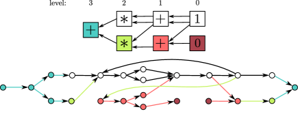
Figure 1: Top: an arithmetic circuit in normal form. Bottom: a DFA (omitting input letters) corresponding to the construction of Prop. 3. Identical colours indicate a correspondence between gates and states.

As an intermediate step of independent interest, we show PosSLP-hardness of a problem about deterministic finite automata (DFAs). Let $\Sigma$ be a finite alphabet and call a function $f:\Sigma\to\mathbb{N}$ a Parikh function. The Parikh image of a word $w\in\Sigma^{*}$ is the Parikh function $f$ such that $f(a)$ is the number of occurrences of $a$ in $w$. We show:

Proposition 3

Given an arithmetic circuit including gate $g$, one can compute in logarithmic space a Parikh function $f$ (in binary encoding) and a DFA $\mathcal{A}$ such that $\mathit{val}(g)$ equals the number of accepting computations in $\mathcal{A}$ that are labelled with words that have Parikh image $f$.

The construction is illustrated in Fig. 1. It is by induction on the levels of the arithmetic circuit. A gate labelled with “+” is simulated by branching into the inductively constructed gadgets corresponding to the gates this gate connects to. Likewise, a gate labelled with “$\ast$” is simulated by sequentially composing the gadgets corresponding to the gates this gate connects to. It is the latter case that may introduce cycles in the structure of the DFA. Building on this construction, by encoding alphabet letters in natural numbers encoded in binary, we then show:

Proposition 4

Given an arithmetic circuit including gate $g$ on odd level $\ell$, one can compute in logarithmic space a cost process $\mathcal{C}$ and $T\in\mathbb{N}$ with $\mathcal{P}(K_{\mathcal{C}}=T)=\mathit{val}(g)/m$, where $m=\exp_{2}(2^{(\ell-1)/2+1}-1)\cdot\exp_{d}(2^{(\ell-1)/2+1}-3)$.

Towards the PosSLP lower bound from Thm. 4.2, given an arithmetic circuit including gates $g_{1},g_{2}$, we use Prop. 4 to construct two cost chains $\mathcal{C}_{1}=(Q,q_{1},t,\Delta)$ and $\mathcal{C}_{2}=(Q,q_{2},t,\Delta)$ and $T_{1},T_{2}\in\mathbb{N}$ such that $\mathcal{P}(K_{\mathcal{C}_{i}}=T_{i})=\mathit{val}(g_{i})/m$ holds for $i\in\{1,2\}$ and for $m\in\mathbb{N}$ as in Prop. 4. Then we compute a number $H\geq T_{2}$ such that $\mathcal{P}(K_{\mathcal{C}_{2}}>H)<1/m$. The representation of $m$ from Prop. 4 is of exponential size. However, using Prop. 2, $H$ depends only logarithmically on $m+1$. We combine $\mathcal{C}_{1}$ and $\mathcal{C}_{2}$ to a cost chain $\mathcal{C}=(Q\uplus\{q_{0}\},q_{0},t,\widetilde{\Delta})$, where $\widetilde{\Delta}$ extends $\Delta$ by $\widetilde{\Delta}(q_{0})(q_{1},H+1)=1/2$ and $\widetilde{\Delta}(q_{0})(q_{2},0)=1/2$. By this construction, the new cost chain $\mathcal{C}$ initially either incurs cost $H+1$ and then emulates $\mathcal{C}_{1}$, or incurs cost $0$ and then emulates $\mathcal{C}_{2}$. Those possibilities have probability $1/2$ each.

Finally, we compute a suitable cost formula $\varphi$ such that we have $\mathit{val}(g_{1})\geq\mathit{val}(g_{2})$ if and only if $\mathcal{P}(K_{\mathcal{C}}\models\varphi)\geq 1/2$, completing the logspace reduction. We remark that the structure of the formula $\varphi$, in particular the number of inequalities, is fixed. Only the involved numbers depend on the concrete instance.

5 Cost Processes

Acyclic Cost Processes.

We now prove that the cost problem for acyclic cost processes is PSpace-complete. The challenging part is to show that PSpace-hardness even holds for atomic cost formulas. For our lower bound, we reduce from a generalisation of the classical SubsetSum problem: Given a tuple $(k_{1},\ldots,k_{n},T)$ of natural numbers with $n$ even, the QSubsetSum problem asks whether the following formula is true:

$$\exists x_{1}\in\{0,1\}\ \forall x_{2}\in\{0,1\}\ \cdots\ \exists x_{n-1}\in\{0,1\}\ \forall x_{n}\in\{0,1\}\ :\ \sum_{1\leq i\leq n}x_{i}k_{i}=T$$

Here, the quantifiers $\mathord{\exists}$ and $\mathord{\forall}$ occur in strict alternation. It is shown in [22, Lem. 4] that QSubsetSum is PSpace-complete. One can think of such a formula as a turn-based game, the QSubsetSum game, played between Player Odd and Player Even. If $i\in\{1,\ldots,n\}$ is odd (even), then turn $i$ is Player Odd’s (Player Even’s) turn, respectively. In turn $i$ the respective player decides to either take $k_{i}$ by setting $x_{i}=1$, or not to take $k_{i}$ by setting $x_{i}=0$. Player Odd’s objective is to make the sum of the taken numbers equal $T$, and Player Even tries to prevent that. If Player Even is replaced by a random player, then Player Odd has a strategy to win with probability $1$ if and only if the given instance is a “yes” instance for QSubsetSum. This gives an easy PSpace-hardness proof for the cost problem with non-atomic cost formulas $\varphi\equiv(x=T)$. In order to strengthen the lower bound to atomic cost formulas $\varphi\equiv(x\leq B)$ we have to give Player Odd an incentive to take numbers $k_{i}$, although she is only interested in not exceeding the budget $B$. This challenge is addressed in our PSpace-hardness proof.

The PSpace-hardness result reflects the fact that the optimal strategy must take the current cost into account, not only the control state, even for atomic cost formulas. This may be somewhat counter-intuitive, as a good strategy should always “prefer small cost”. But if there always existed a strategy depending only on the control state, one could guess this strategy in NP and invoke the PP-result of Sec. 4 in order to obtain an NP${}^{\text{PP}}$ algorithm, implying NP${}^{\text{PP}}$ = PSpace and hence a collapse of the counting hierarchy.

Indeed, for a concrete example, consider the acyclic cost process with $Q=\{q_{0},q_{1},t\}$, and $\mathit{En}(q_{0})=\{a\}$ and $\mathit{En}(q_{1})=\{a_{1},a_{2}\}$, and $\Delta(q_{0},a)(q_{1},+1)=\frac{1}{2}$ and $\Delta(q_{0},a)(q_{1},+3)=\frac{1}{2}$ and $\Delta(q_{1},a_{1})(t,+3)=1$ and $\Delta(q_{1},a_{2})(t,+6)=\frac{1}{2}$ and $\Delta(q_{1},a_{2})(t,+1)=\frac{1}{2}$. Consider the atomic cost formula $\varphi\equiv(x\leq 5)$. An optimal scheduler $\sigma$ plays $a_{1}$ in $(q_{1},1)$ and $a_{2}$ in $(q_{1},3)$, because additional cost $3$, incurred by $a_{1}$, is fine in the former but not in the latter configuration. For this scheduler $\sigma$ we have $\mathcal{P}_{\sigma}(K\models\varphi)=\frac{3}{4}$.

Theorem 5.1

The cost problem for acyclic cost processes is in PSpace. It is PSpace-hard, even for atomic cost formulas.

Proof (sketch)

To prove membership in PSpace, we consider a procedure Opt that, given $(q,c)\in Q\times\mathbb{N}$ as input, computes the optimal (i.e., maximised over all schedulers) probability $p_{q,c}$ that starting from $(q,c)$ one reaches $(t,d)$ with $d\models\varphi$. The following procedure characterisation of $p_{q,c}$ for $q\neq t$ is crucial for Opt$(q,c)$:

$$p_{q,c}=\max_{a\in\mathit{En}(q)}\sum_{q^{\prime}\in Q}\sum_{k\in\mathbb{N}}\Delta(q,a)(q^{\prime},k)\cdot p_{q^{\prime},c+k}$$

So Opt$(q,c)$ loops over all $a\in\mathit{En}(q)$ and all $(q^{\prime},k)\in Q\times\mathbb{N}$ with $\Delta(q,a)(q^{\prime},k)>0$ and recursively computes $p_{q^{\prime},c+k}$. Since the cost process is acyclic, the height of the recursion stack is at most $|Q|$. The representation size of the probabilities that occur in that computation is polynomial. To see this, consider the product $D$ of the denominators of the probabilities occurring in the description of $\Delta$. The encoding size of $D$ is polynomial. All probabilities occurring during the computation are integer multiples of $1/D$. Hence computing $\textsc{Opt}(q_{0},0)$ and comparing the result with $\tau$ gives a PSpace procedure.

For the lower bound we reduce the QSubsetSum problem, defined above, to the cost problem for an atomic cost formula $x\leq B$. Given an instance $(k_{1},\ldots,k_{n},T)$ with $n$ is even of the QSubsetSum problem, we construct an acyclic cost process $\mathcal{C}=(Q,q_{0},t,A,\mathit{En},\Delta)$ as follows. We take $Q=\{q_{0},q_{2},\ldots,q_{n-2},q_{n},t\}$. Those control states reflect pairs of subsequent turns that the QSubsetSum game can be in. The transition rules $\Delta$ will be set up so that probably the control states $q_{0},q_{2},\ldots,q_{n},t$ will be visited in that order, with the (improbable) possibility of shortcuts to $t$. For even $i$ with $0\leq i\leq n{-}2$ we set $\mathit{En}(q_{i})=\{a_{0},a_{1}\}$. These actions correspond to Player Odd’s possible decisions of not taking, respectively taking $k_{i+1}$. Player Even’s response is modelled by the random choice of not taking, respectively taking $k_{i+2}$ (with probability $1/2$ each). In the cost process, taking a number $k_{i}$ corresponds to incurring cost $k_{i}$. We also add an additional cost $\ell$ in each transition. Therefore we define our cost problem to have the atomic formula $x\leq B$ with $B:=(n/2)\cdot\ell+T$. For some large number $M\in\mathbb{N}$, formally defined in App. 0.D, we set for all even $i\leq n{-}2$ and for $j\in\{0,1\}$:

$$\Delta(q_{i},a_{j})(q_{i+2},\ell+j\cdot k_{i+1}) =(1/2)\cdot\left(1-(\ell+j\cdot k_{i+1})/M\right)$$

$$\Delta(q_{i},a_{j})(t,\ell+j\cdot k_{i+1}) =(1/2)\cdot(\ell+j\cdot k_{i+1})/M$$

$$\Delta(q_{i},a_{j})(q_{i+2},\ell+j\cdot k_{i+1}+k_{i+2}) =(1/2)\cdot\left(1-(\ell+j\cdot k_{i+1}+k_{i+2})/M\right)$$

$$\Delta(q_{i},a_{j})(t,\ell+j\cdot k_{i+1}+k_{i+2}) =(1/2)\cdot(\ell+j\cdot k_{i+1}+k_{i+2})/M$$

So with high probability the MDP transitions from $$q_{i} q_{i+2} \ell \ell+k_{i+1} \ell+k_{i+2} \ell+k_{i+1}+k_{i+2} t B q_{n}$$ to , and cost , , , is incurred, depending on the scheduler’s (i.e., Player Odd’s) actions and on the random (Player Even) outcome. But with a small probability, which is proportional to the incurred cost, the MDP transitions to , which is a “win” for the scheduler as long as the accumulated cost is within budget . We make sure that the scheduler loses if is reached:

$$\Delta(q_{n},a)(t,B{+}1) =1\qquad\text{with $\mathit{En}(q_{n})=\{a\}$}$$

The MDP is designed so that the scheduler probably “loses” (i.e., exceeds the budget $B$); but whenever cost $k$ is incurred, a winning opportunity with probability $k/M$ arises. Since $1/M$ is small, the overall probability of winning is approximately $C/M$ if total cost $C\leq B$ is incurred. In order to maximise this chance, the scheduler wants to maximise the total cost without exceeding $B$, so the optimal scheduler will target $B$ as total cost.

The values for $\ell$, $M$ and $\tau$ need to be chosen carefully, as the overall probability of winning is not exactly the sum of the probabilities of the individual winning opportunities. By the “union bound”, this sum is only an upper bound, and one needs to show that the sum approximates the real probability closely enough. ∎

General Cost Processes.

We show the following theorem:

Theorem 5.2

The cost problem is EXP-complete.

Proof (sketch)

The EXP upper bound was stated in Prop. 1. Regarding hardness, we build upon countdown games, “a simple class of turn-based 2-player games with discrete timing” [12]. Deciding the winner in a countdown game is EXP-complete [12]. Albeit non-stochastic, countdown games are very close to our model: two players move along edges of a graph labelled with positive integer weights and thereby add corresponding values to a succinctly encoded counter. Player 1’s objective is to steer the value of the counter to a given number $T\in\mathbb{N}$, and Player 2 tries to prevent that. Our reduction from countdown games in App. 0.D requires a small trick, as in our model the final control state $t$ needs to be reached with probability 1 regardless of the scheduler, and furthermore, the scheduler attempts to achieve the cost target $T$ when and only when the control state $t\in Q$ is visited. ∎

The Cost-Utility Problem.

MDPs with two non-negative and non-decreasing integer counters, viewed as cost and utility, respectively, were considered in [2, 3]. Specifically, those works consider problems such as computing the minimal cost $C$ such that the probability of gaining at least a given utility $U$ is at least $\tau$. Possibly the most fundamental of those problems is the following: the cost-utility problem asks, given an MDP with both cost and utility, and numbers $C,U\in\mathbb{N}$, whether one can, with probability 1, gain utility at least $U$ using cost at most $C$. Using essentially the proof of Thm. 5.2 we show:

Corollary 1

The cost-utility problem is EXP-complete.

The Universal Cost Problem.

We defined the cost problem so that it asks whether there exists a scheduler $\sigma$ with $\mathcal{P}_{\sigma}(K_{\mathcal{C}}\models\varphi)\geq\tau$. A natural variant is the universal cost problem, which asks whether for all schedulers $\sigma$ we have $\mathcal{P}_{\sigma}(K_{\mathcal{C}}\models\varphi)\geq\tau$. Here the scheduler is viewed as an adversary which tries to prevent the satisfaction of $\varphi$. Clearly, for cost chains the cost problem and the universal cost problem are equivalent. Moreover, Thms. 5.1 and 5.2 hold analogously in the universal case.

Theorem 5.3

The universal cost problem for acyclic cost processes is in PSpace. It is PSpace-hard, even for atomic cost formulas. The universal cost problem is EXP-complete.

Proof (sketch)

The universal cost problem and the complement of the cost problem (and their acyclic versions) are interreducible in logarithmic space by essentially negating the cost-formulas. The only problem is that if $\varphi$ is an atomic cost formula, then $\neg\varphi$ is not an atomic cost formula. However, the PSpace-hardness proof from Thm. 5.1 can be adapted, cf. App. 0.E. ∎

6 Conclusions and Open Problems

In this paper we have studied the complexity of analysing succinctly represented stochastic systems with a single non-negative and only increasing integer counter. We have improved the known complexity bounds significantly. Among other results, we have shown that the cost problem for Markov chains is in PSpace and both hard for PP and the PosSLP problem. It would be fascinating and potentially challenging to prove either PSpace-hardness or membership in the counting hierarchy: the problem does not seem to lend itself to a PSpace-hardness proof, but the authors are not aware of natural problems, except BitSLP [1], that are in the counting hierarchy and known to be hard for both PP and PosSLP.

Regarding acyclic and general MDPs, we have proved PSpace-completeness and EXP-completeness, respectively. Our results leave open the possibility that the cost problem for atomic cost formulas is not EXP-hard and even in PSpace. The technique described in the proof sketch of Thm. 5.1 cannot be applied to general cost processes, because there we have to deal with paths of exponential length, which, informally speaking, have double-exponentially small probabilities. Proving hardness in an analogous way would thus require probability thresholds $\tau$ of exponential representation size.

Acknowledgements.

The authors would like to thank Andreas Göbel for valuable hints, Christel Baier and Sascha Klüppelholz for thoughtful feedback on an earlier version of this paper, and the anonymous referees for their helpful comments.

Appendix 0.A Proofs of Section 2

Proposition 5

Let $\mathcal{C}$ be a cost process, $\varphi$ a cost formula with $n_{0}\not\models\varphi$ and $n_{1}\models\varphi$ for some $n_{0},n_{1}\in\mathbb{N}$, and $\tau\in[0,1]$. One can construct in logarithmic space a cost process $\mathcal{C}^{\prime}$ such that the following holds: There is a scheduler $\sigma$ for $\mathcal{C}$ with $\mathcal{P}_{\sigma}(K_{\mathcal{C}}\models\varphi)\geq\tau$ if and only if there is a scheduler $\sigma^{\prime}$ for $\mathcal{C}^{\prime}$ with $\mathcal{P}_{\sigma^{\prime}}(K_{\mathcal{C}^{\prime}}\models\varphi)\geq 1/2$. Moreover, $\mathcal{C}^{\prime}$ is a cost chain if $\mathcal{C}$ is.

Proof

Let $\tau<1/2$. Define $p:=(1/2-\tau)/(1-\tau)$. To construct $\mathcal{C}^{\prime}$ from $\mathcal{C}$, add a new initial state $s_{00}$ with exactly one enabled action, say $a$, and set $\Delta(s_{00},a)(t,n_{1})=p$ and $\Delta(s_{00},a)(s_{0},0)=1-p$. In a straightforward sense any scheduler for $\mathcal{C}$ can be viewed as a scheduler for $\mathcal{C}^{\prime}$ and vice versa. Thus for any scheduler $\sigma$ we have $\mathcal{P}^{\prime}_{\sigma}(K\models\varphi)=p+(1-p)\cdot\mathcal{P}_{\sigma}(K\models\varphi)$. The statement of the proposition now follows from a simple calculation.

Now let $\tau>1/2$. Define $p:=1/(2\tau)$. In a similar way as before, add a new initial state $s_{00}$ with exactly one enabled action $a$, and set $\Delta(s_{00},a)(t,n_{0})=1-p$ and $\Delta(s_{00},a)(s_{0},0)=p$. Thus we have $\mathcal{P}^{\prime}_{\sigma}(K\models\varphi)=p\cdot\mathcal{P}_{\sigma}(K\models\varphi)$, and the statement of the proposition follows. ∎

Appendix 0.B Proofs of Section 3

In this section we prove Prop. 2 from the main text:

Proposition 2. Suppose $0\leq\tau<1$. Let $p_{\mathit{min}}$ be the smallest non-zero probability and $k_{\mathit{max}}$ be the largest cost in the description of the cost process. Then $\mathcal{P}_{\sigma}(K\leq B)\geq\tau$ holds for all schedulers $\sigma$, where

$$B:=k_{\mathit{max}}\cdot\left\lceil|Q|\cdot\left(-\ln(1-\tau)/p_{\mathit{min}}^{|Q|}\ +\ 1\right)\right\rceil\;.$$

Proof

Define $n:=|Q|$. If $p_{\mathit{min}}=1$, then by our assumption on the almost-sure reachability of $t$, the state $t$ will be reached within $n$ steps, and the statement of the proposition follows easily. So we can assume $p_{\mathit{min}}<1$ for the rest of the proof.

Let $j\in\mathbb{N}$ be the smallest integer with

$$j\geq n\cdot\left(\frac{-\ln(1-\tau)}{p_{\mathit{min}}^{n}}+1\right)\,.$$

It follows:

$$\left\lfloor\frac{j}{n}\right\rfloor \geq\frac{-\ln(1-\tau)}{p_{\mathit{min}}^{n}}$$

$$\geq\frac{\ln(1-\tau)}{\ln(1-p_{\mathit{min}}^{n})} x\leq-\ln(1-x) x<1$$ (as for ) (1)

For $i\in\mathbb{N}$ and $q\in Q$ and a scheduler $\sigma$, define $p_{i}(q,\sigma)$ as the probability that, if starting in $q$ and using the scheduler $\sigma$, more than $i$ steps are required to reach the target state $t$. Define $p_{i}:=\max\{p_{i}(q,\sigma):q\in Q,\ \sigma\text{ a scheduler}\}$. By our assumption on the almost-sure reachability of $t$, regardless of the scheduler, there is always a path to $t$ of length at most $n$. This path has probability at least $p_{\mathit{min}}^{n}$, so $p_{n}\leq 1-p_{\mathit{min}}^{n}$. If a path of length $\ell\cdot n$ does not reach $t$, then none of its $\ell$ consecutive blocks of length $n$ reaches $t$, so we have $p_{\ell\cdot n}\leq p_{n}^{\ell}$. Hence we have:

$$p_{j} \leq p_{\lfloor j/n\rfloor\cdot n} p_{i}\geq p_{i+1} i\in\mathbb{N}$$ (as for all )

$$\leq p_{n}^{\lfloor j/n\rfloor}$$ (as argued above)

$$\leq(1-p_{\mathit{min}}^{n})^{\lfloor j/n\rfloor}$$ (as argued above)

$$=\exp\big{(}\ln(1-p_{\mathit{min}}^{n})\cdot\lfloor j/n\rfloor\big{)}$$

$$\leq 1-\tau$$ (by (1)) (2)

Denote by $T$ the random variable that assigns to a run the “time” (i.e., the number of steps) to reach $t$ from $s_{0}$. Then we have for all schedulers $\sigma$:

$$\mathcal{P}_{\sigma}(K\leq B) =\mathcal{P}_{\sigma}(K\leq j\cdot k_{\mathit{max}}) B$$ (by the definition of )

$$\geq P_{\sigma}(T\leq j) k_{\mathit{max}}$$ (each step costs at most )

$$=1-P_{\sigma}(T>j)$$

$$\geq 1-p_{j} T p_{i}$$ (by the definition of and )

$$\geq\tau$$ (by (2)) ,

as claimed. ∎

Appendix 0.C Proofs of Section 4

0.C.1 Proof of Thm. 4.1

In this section we prove Thm. 4.1 from the main text:

Theorem 4.1. The cost problem for acyclic cost chains is in PP. It is PP-hard under polynomial-time Turing reductions, even for atomic cost formulas.

Proof

First we prove membership in PP. Recall from the main text that the class PP can be defined as the class of languages $L$ that have a probabilistic polynomial-time bounded Turing machine $M_{L}$ such that for all words $x$ one has $x\in L$ if and only if $M_{L}$ accepts $x$ with probability at least $1/2$, see [10] and note that PP is closed under complement [10]. By Prop. 5 it suffices to consider an instance of the cost problem with $\tau=1/2$. The problem can be decided by a probabilistic Turing machine that simulates the cost chain as follows: The Turing machine keeps track of the control state and the cost, and branches according to the probabilities specified in the cost chain. It accepts if and only if the accumulated cost satisfies $\varphi$. Note that the acyclicity of the cost chain guarantees the required polynomial time bound. This proof assumes that the probabilistic Turing machine has access to coins that are biased according to the probabilities in the cost chain. As we show in [11, Lem. 1], this can indeed be assumed for probabilistic polynomial-time bounded Turing machines.

As stated in the main text, the lower bound follows from combining the result from [14, Prop. 4] with [11, Thm. 3]. ∎

0.C.2 Proof of Thm. 4.2

In this section we prove Thm. 4.2 from the main text:

Theorem 4.2. The cost problem for cost chains is in PSpace and hard for PosSLP.

First we give details on the upper bound. Then we provide proofs of the statements from the main text that pertain to the PosSLP lower bound.

0.C.2.1 Proof of the Upper Bound in Thm. 4.2.

We show that the cost problem for cost chains is in PSpace. As outlined in the main text we use the fact that PSpace equals probabilistic PSpace. The cost problem for cost chains is in this class. This can be shown in the same way as we showed in Thm. 4.1 that the cost problem for acyclic cost chains is in PP. More concretely, given an instance of the cost problem for cost chains, we construct in logarithmic space a probabilistic PSpace Turing machine that simulates the cost chain and accepts if and only if the accumulated cost $K$ satisfies the given cost formula.

The fact that (this definition of) probabilistic PSpace equals PSpace was first proved in [20]. A simpler proof can be obtained using a result by Ladner [13] that states that #PSpace equals FPSpace, see [13] for definitions. This was noted implicitly, e.g., in [15, Thm. 5.2]. We remark that the class PPSpace defined in [16] also equals PSpace, but its definition (which is in terms of stochastic games) is different.

0.C.2.2 Proof of Prop. 3.

Here, we give a formal definition and proof of the construction outlined in the main text which allows for computing the value of an arithmetic circuit as the number of paths in a DFA with a certain Parikh image. First, we formally define the notations informally used in the main text.

We first introduce arithmetic circuits and at the same time take advantage of a normal form that avoids gates labelled with “$-$”. This normal form was established in the proof of [9, Thm. 5.2]. An arithmetic circuit is a directed acyclic graph $G=(V,E)$ whose leaves are labelled with constants “$0$” and “$1$”, and whose vertices are labelled with operators “$+$” and “$\ast$”. Subsequently, we refer to the elements of $V$ as gates. With every gate we associate a level starting at $0$ with leaves. For levels greater than zero, gates on odd levels are labelled with “$+$” and on even levels with “$\ast$”. Moreover, all gates on a level greater than zero have exactly two incoming edges from the preceding level. The upper part of Fig. 1 illustrates an arithmetic circuit in this normal form. We can associate with every gate $v\in V$ a non-negative integer $\mathit{val}(v)$ in the obvious way. In this form, the PosSLP problem asks, given an arithmetic circuit $G=(V,E)$ and two gates $v_{1},v_{2}\in V$, whether $\mathit{val}(v_{1})\geq\mathit{val}(v_{2})$ holds.

Regarding the relevant definitions of Parikh images, let $\mathcal{A}=(Q,\Sigma,\Delta)$ be a DFA such that $Q$ is a finite set of control states, $\Sigma=\{a_{1},\ldots,a_{k}\}$ is a finite alphabet, and $\Delta\subseteq Q\times\Sigma\times Q$ is the set of transitions. A path $\pi$ in $\mathcal{A}$ is a sequence of transitions $\pi=\delta_{1}\cdots\delta_{n}\in\Delta^{*}$ such that $\delta_{i}=(q_{i},a_{i},q_{i}^{\prime})$ and $\delta_{i+1}=(q_{i+1},a_{i+1},q_{i+1}^{\prime})$ implies $q_{i}^{\prime}=q_{i+1}$ for all $1\leq i<n$. Let $q,q^{\prime}\in Q$, we denote by $\Pi(\mathcal{A},q,q^{\prime})$ the set of all paths starting in $q$ and ending in $q^{\prime}$. In this paper, a Parikh function is a function $f:\Sigma\to\mathbb{N}$. The Parikh image of a path $\pi$, denoted $\mathit{parikh}(\pi)$, is the unique Parikh function counting for every $a\in\Sigma$ the number of times $a$ occurs on a transition in $\pi$.

The following statement of Prop. 3 makes the one given in the main text more precise.

Proposition 3. Let $G=(V,E)$ be an arithmetic circuit and $v\in V$. There exists a log-space computable DFA $\mathcal{A}=(Q,\Sigma,\Delta)$ with distinguished control states $q,q^{\prime}\in Q$ and a Parikh function $f:\Sigma\to\mathbb{N}$ such that

$$\mathit{val}(v)=|\{\pi\in\Pi(\mathcal{A},q,q^{\prime}):\mathit{parikh}(\pi)=f\}|.$$

Proof

We construct $\mathcal{A}$ by induction on the number of levels of $V$. For every level $i$, we define an alphabet $\Sigma_{i}$ and a Parikh function $f_{i}:\Sigma_{i}\to\mathbb{N}$. As an invariant, $\Sigma_{i}\subseteq\Sigma_{i+1}$ holds for all levels $i$. Subsequently, denote by $V(i)$ all gates on level $i$. For every $v\in V(i)$, we define a DFA $\mathcal{A}_{v}$ such that each $\mathcal{A}_{v}$ has two distinguished control locations $\mathit{in}(\mathcal{A}_{v})$ and $\mathit{out}(\mathcal{A}_{v})$. The construction is such that

$$\mathit{val}(v)=|\{\pi\in\Pi(\mathcal{A}_{v},\mathit{in}(\mathcal{A}_{v}),\mathit{out}(\mathcal{A}_{v})):\mathit{parikh}(\pi)=f_{i}\}|.$$ (3)

For technical convenience, we allow transitions to be labelled with subsets $S\subseteq\Sigma$ which simply translates into an arbitrary chain of transitions such that each $a\in S$ occurs exactly once along this chain. We now proceed with the details of the construction starting with gates on level $0$.

With no loss of generality we may assume that there are two gates $v$ and $w$ on level $0$ labelled with $0$ and $1$, respectively. Let $\Sigma_{0}=\{a\}$ for some letter $a$. The DFA $\mathcal{A}_{v}$ and $\mathcal{A}_{w}$ over $\Sigma_{0}$ is defined as follows: $\mathcal{A}_{w}$ has a single transition connecting $\mathit{in}(\mathcal{A}_{w})$ with $\mathit{out}(\mathcal{A}_{w})$ labelled with $a$, whereas $\mathcal{A}_{v}$ does not have this transition. Setting $f_{0}(a)=1$, it is easily checked that (3) holds for those DFA.

For level $i+1$, we define $\Sigma_{i+1}=\Sigma_{i}\uplus\{a_{v},b_{v},c_{v}:v\in V(i+1)\}$. Let $v\in V(i+1)$ be a gate on level $i+1$ such that $v$ has incoming edges from $u$ and $w$. Let $\mathcal{A}_{u}=(Q_{u},\Sigma_{i},\Delta_{u})$ and $\mathcal{A}_{w}=(Q_{w},\Sigma_{i},\Delta_{w})$ be the DFA representing $u$ and $w$. Let $Q_{v}$ be a set of fresh control states. We define $\mathcal{A}_{v}=(Q_{v}\cup Q_{u}\cup Q_{w},\Sigma_{i+1},\Delta_{v}\cup\Delta_{u}\cup\Delta_{w})$. The particularities of the construction depend on the type of $v$.

If $i+1$ is odd, i.e., the gates on this level are labelled with “+”, then apart from the control states $\mathit{in}(\mathcal{A}_{v})$ and $\mathit{out}(\mathcal{A}_{v})$, the set $Q_{v}$ contains three additional control states $q,q_{1},q_{2}$. Further we set $\Delta_{v}=\{\delta_{1},\ldots,\delta_{7}\}$ such that

• $\delta_{1}=(\mathit{in}(\mathcal{A}_{v}),S_{v},q)$, where $S_{v}=\{a_{w},b_{w},c_{w}:w\in V(i+1),v\neq w\}$;

• $\delta_{2}=(q,a_{v},q_{1})$ and $\delta_{3}=(q,b_{v},q_{2})$;

• $\delta_{4}=(q_{1},b_{v},\mathit{in}(\mathcal{A}_{u}))$ and $\delta_{5}=(q_{2},a_{v},\mathit{in}(\mathcal{A}_{w}))$; and

• $\delta_{6}=(\mathit{out}(\mathcal{A}_{u}),c_{v},\mathit{out}(\mathcal{A}))$ and $\delta_{7}=(\mathit{out}(\mathcal{A}_{w}),c_{v},\mathit{out}(\mathcal{A}))$.

Informally speaking, we simply branch at $q$ into $\mathcal{A}_{u}$ and $\mathcal{A}_{w}$, and this in turn enforces that the number of paths in $\Pi(\mathcal{A}_{v},\mathit{in}(\mathcal{A}_{v}),\mathit{out}(\mathcal{A}_{v}))$ on which $a_{v}$ occurs once equals the sum of $\mathit{val}(u)$ and $\mathit{val}(w)$. The reason behind using both $a_{v}$ and $b_{v}$ is that it ensures that the case $u=w$ is handled correctly. Setting $f_{i+1}(a)=1$ if $a\in\Sigma_{i+1}\setminus\Sigma_{i}$, and $f_{i+1}(a)=f_{i}(a)$ otherwise, we consequently have that (3) holds since

$$\hskip 14.22636pt|\{\pi\in\Pi(\mathcal{A}_{v},\mathit{in}(\mathcal{A}_{v}),\mathit{out}(\mathcal{A}_{v})):\mathit{parikh}(\pi)=f_{i+1}\}|$$

$$=|\{\pi\in\Pi(\mathcal{A}_{u},\mathit{in}(\mathcal{A}_{u}),\mathit{out}(\mathcal{A}_{u})):\mathit{parikh}(\pi)=f_{i}\}|+\mbox{}$$

$$\qquad\mbox{}+|\{\pi\in\Pi(\mathcal{A}_{w},\mathit{in}(\mathcal{A}_{w}),\mathit{out}(\mathcal{A}_{w})):\mathit{parikh}(\pi)=f_{i}\}|$$

$$=\mathit{val}(u)+\mathit{val}(w)$$

$$=\mathit{val}(v).$$

The case of $i+1$ being even can be handled analogously, but instead of using branching we use sequential composition in order to simulate the computation of a gate labelled with “$\ast$”. Apart from the control states $\mathit{in}(\mathcal{A}_{v})$ and $\mathit{out}(\mathcal{A}_{v})$, the set $Q_{v}$ contains an additional control state $q$. Further we set $\Delta_{v}=\{\delta_{1},\ldots,\delta_{4}\}$ such that

• $\delta_{1}=(\mathit{in}(\mathcal{A}_{v}),S_{v},q)$, where $S_{v}=\{a_{w},b_{w},c_{w}:w\in V(i+1),v\neq w\}$;

• $\delta_{2}=(q,a_{v},\mathit{in}(\mathcal{A}_{u}))$;

• $\delta_{3}=(\mathit{out}(\mathcal{A}_{u}),b_{v},\mathit{in}(\mathcal{A}_{w}))$; and

• $\delta_{4}=(\mathit{out}(\mathcal{A}_{w}),c_{v},\mathit{out}(\mathcal{A}_{v}))$.

A difference to the case where $i+1$ is odd is that via the definition of $f_{i+1}$ we have to allow for paths that can traverse both $\mathcal{A}_{u}$ and $\mathcal{A}_{w}$. Consequently, we define $f_{i+1}(a)=1$ if $a\in\Sigma_{i+1}\setminus\Sigma_{i}$, and $f_{i+1}(a)=2f_{i}(a)$ otherwise. Similarly as above, (3) holds since

$$\hskip 14.22636pt|\{\pi\in\Pi(\mathcal{A}_{v},\mathit{in}(\mathcal{A}_{v}),\mathit{out}(\mathcal{A}_{v})):\mathit{parikh}(\pi)=f_{i+1}\}|$$

$$=|\{\pi\in\Pi(\mathcal{A}_{u},\mathit{in}(\mathcal{A}_{u}),\mathit{out}(\mathcal{A}_{u})):\mathit{parikh}(\pi)=f_{i}\}|\cdot\mbox{}$$

$$\qquad\mbox{}\cdot|\{\pi\in\Pi(\mathcal{A}_{w},\mathit{in}(\mathcal{A}_{w}),\mathit{out}(\mathcal{A}_{w})):\mathit{parikh}(\pi)=f_{i}\}|$$

$$=\mathit{val}(u)\cdot\mathit{val}(w)$$

$$=\mathit{val}(v).$$

Due to the inductive nature of the construction, the cautious reader may on the first sight cast doubt that the computation of $\mathcal{A}_{v}$ and $f$ can be performed in logarithmic space. However, a closer look reveals that the graph underlying $\mathcal{A}_{v}$ has a simple structure and its list of edges can be constructed without prior knowledge of the DFA on lower levels. Likewise, even though $f$ contains numbers which are exponential in the number of levels of $G$, the structure of $f$ is simple and only contains numbers which are powers of two, and hence $f$ is computable in logarithmic space as well.∎

0.C.2.3 Proof of Prop. 4.

The following statement of Prop. 4 makes the one given in the main text more precise.

Proposition 4. Let $G=(V,E)$ be an arithmetic circuit. Let $v\in V$ be a gate on level $\ell$ with odd $\ell$. There exist a log-space computable cost process $\mathcal{C}$ and $T\in\mathbb{N}$ with $\mathcal{P}(K_{\mathcal{C}}=T)=\mathit{val}(v)/m$, where $m=\exp_{2}(2^{(\ell-1)/2+1}-1)\cdot\exp_{d}(2^{(\ell-1)/2+1}-3)\,.$

For a clearer proof structure we define an intermediate formalism between DFA and cost chains. A typed cost chain $\mathcal{T}=(Q,q_{0},t,\Gamma,\Delta)$ is similar to a cost chain, but with costs (i.e., natural numbers) replaced with functions $\Gamma\to\mathbb{N}$. The intuition is that instead of a single cost, a typed cost chain keeps track of several types of cost, and each type is identified with a symbol from $\Gamma$. More precisely, $Q$ is a finite set of control states, $q_{0}\in Q$ is the initial control state, $t$ is the target control state, $\Gamma$ is a finite alphabet, and $\Delta:Q\to\mathit{dist}(Q\times\mathbb{N}^{\Gamma})$ is a probabilistic transition function.

A typed cost chain $\mathcal{T}$ induces a Markov chain in the same way as a cost chain does, but the state space is $Q\times\mathbb{N}^{\Gamma}$ rather than $Q\times\mathbb{N}$. Formally, $\mathcal{T}$ induces the Markov chain $\mathcal{D}_{\mathcal{T}}=(Q\times\mathbb{N}^{\Gamma},(q_{0},\mathbf{0}),\delta)$, where by $\mathbf{0}$ we mean the function $c:\Gamma\to\mathbb{N}$ with $c(a)=0$ for all $a\in\Gamma$, and $\delta(q,c)(q^{\prime},c^{\prime})=\Delta(q)(q^{\prime},c^{\prime}-c)$ holds for all $q,q^{\prime}\in Q$ and $c,c^{\prime}\in\mathbb{N}^{\Gamma}$, where by $c^{\prime}-c$ we mean $c^{\prime\prime}:\Gamma\to\mathbb{N}$ with $c^{\prime\prime}(a)=c^{\prime}(a)-c(a)$ for all $a\in\Gamma$. As before, we assume that the target control state $t$ is almost surely reached. We write $K_{\mathcal{T}}$ for the (multi-dimensional) random variable that assigns a run in $\mathcal{D}_{\mathcal{T}}$ the typed cost $c:\Gamma\to\mathbb{N}$ that is accumulated upon reaching $t$.

Lemma 1

Let $G=(V,E)$ be an arithmetic circuit. Let $v\in V$ be a gate on level $\ell$ with odd $\ell$. Let $d=|V|+1$. There exist a log-space computable typed cost chain $\mathcal{T}=(Q,q_{0},t,\Gamma,\Delta)$ and $c:\Gamma\to\mathbb{N}$ such that $\mathcal{P}(K_{\mathcal{T}}=c)=\mathit{val}(v)/m$, where

$$m=\exp_{2}(2^{(\ell-1)/2+1}-1)\cdot\exp_{d}(2^{(\ell-1)/2+1}-3)\,.$$

Proof

With no loss of generality we may assume that the maximum level of $V$ is $\ell$ and that $v$ is the only gate on level $\ell$. The idea is to translate the DFA obtained in Prop. 3 into a suitable typed cost chain. Subsequently, we refer to the terminology used in the proof of Prop. 3.

Let $\mathcal{A}=(Q,\Sigma,\Delta)$ be the DFA, $q_{0}=\mathit{in}(\mathcal{A}_{v})$, $t=\mathit{out}(\mathcal{A}_{v})$, and $f:\Sigma\to\mathbb{N}$ be the Parikh function obtained from Prop. 3. We define $\Gamma=\Sigma\uplus\{e_{j}:1\leq j\leq d\}$ and alter $\mathcal{A}$ as follows:

• for the gate $w\in V$ on level 0 labelled with 0, we add an edge from $\mathit{in}(\mathcal{A}_{w})$ to $t$ labelled with $e_{1}$; and

• for every $w\in V$ such that $w\neq v$, we add $k$ edges labelled with $e_{1},\ldots,e_{k}$ from $\mathit{out}(\mathcal{A}_{w})$ to $t$, where $k$ is the difference between $d$ and the number of outgoing edges from $\mathit{out}(\mathcal{A}_{w})$.

The DFA $\mathcal{A}^{\prime}=(Q,\Gamma,\Delta^{\prime})$ obtained from this construction has the property that $t$ can be reached from any control state, and that the number of outgoing edges from any $\mathit{out}(\mathcal{A}_{w})$ for $w\neq v$ is uniform. Finally, we define $c:\Gamma\to\mathbb{N}$ such that $c$ coincides with $f$ for all $a\in\Sigma$ and $c(e_{j})=0$ for all $1\leq j\leq k$. The intuition behind the $e_{j}$ is that they indicate errors, and once an edge with an $e_{j}$ is traversed it is impossible to reach $t$ with Parikh image $c$. Thus, in particular property (3) is preserved in $\mathcal{A}^{\prime}$.

We now transform $\mathcal{A}^{\prime}$ into a typed cost chain $\mathcal{T}$. Subsequently, for $a\in\Gamma$ let $c_{a}:\Gamma\to\{0,1\}$ be the function such that $c_{a}(b)=1$ if $b=a$ and $c_{a}(b)=0$ otherwise. For our transformation, we perform the following steps:

• every alphabet letter $a\in\Gamma$ labelling a transition of $\mathcal{A}^{\prime}$ is replaced by $c_{a}$;

• the probability distribution over edges is chosen uniformly; and

• a self-loop labelled with $\mathbf{0}$ and probability 1 is added at $t$.

We observe that the transition probabilities of $\mathcal{T}$ are either $1/d$, $1/2$ or $1$. Since $t$ can be reached from any control state, it is eventually reached with probability $1$.

For every level $i$ and every $w\in V(i)$, let $p_{w}$ denote the probability that, starting from $\mathit{in}(\mathcal{A}_{w})$, the control state $\mathit{out}(\mathcal{A}_{w})$ is reached and typed cost $c_{i}$ is accumulated. Here, $c_{i}$ refers to the Parikh function $f_{i}$ constructed in the proof of Prop. 3, where we assert that $c_{i}(a)=0$ for all $a\in\Gamma$ on which the “original” $f_{i}$ is undefined. Since $t=\mathit{out}(\mathcal{A}_{v})$ is almost surely reached from $q_{0}=\mathit{in}(\mathcal{A}_{v})$, we have $p_{v}=\mathcal{P}(K_{\mathcal{T}}=c_{\ell})$. So in order to prove the lemma, it suffices to prove for all $i\in\mathbb{N}$:

$$p_{w}=\frac{\mathit{val}(w)}{m(i)}\qquad\text{for all $w\in V(i)$,}$$

where

$$m(i) =\left\{\begin{array}[]{ll}\exp_{2}(2^{i/2+1}-2)\cdot\exp_{d}(2^{i/2+1}-4)&\text{ if }i\text{ is even}\\ \exp_{2}(2^{(i-1)/2+1}-1)\cdot\exp_{d}(2^{(i-1)/2+1}-3)&\text{ if }i\text{ is odd\,.}\end{array}\right.$$

We proceed by induction on the level $i$. Let $i=0$. If $w$ is labelled with $1$ then there is exactly one outgoing transition from $\mathit{in}(\mathcal{A}_{w})$, and this transition goes to $\mathit{out}(\mathcal{A}_{w})$ and incurs cost $c_{0}$. So we have $p_{w}=1$ as required. If $w$ is labelled with $0$, then the only outgoing transition from $\mathit{in}(\mathcal{A}_{w})$ incurs cost $c$ with $c(e_{1})=1$, hence $p_{w}=0$.

For the induction step, let $i\geq 0$. Let $w\in V(i+1)$ and let $u,u^{\prime}\in V(i)$ be the gates connected to $w$. If $i+1$ is odd then $w$ is labelled with “+”, and by the construction of $\mathcal{A}_{w}$ and the transformation above we have

$$p_{w} =\frac{1}{2}\cdot\frac{1}{d}\cdot(p_{u}+p_{u^{\prime}})$$

$$=\frac{1}{2}\cdot\frac{1}{d}\cdot\frac{\mathit{val}(u)+\mathit{val}(u^{\prime})}{\exp_{2}(2^{i/2+1}-2)\cdot\exp_{d}(2^{i/2+1}-4)}$$ by the ind. hypoth.

$$=\frac{\mathit{val}(u)+\mathit{val}(u^{\prime})}{\exp_{2}(2^{i/2+1}-1)\cdot\exp_{d}(2^{i/2+1}-3)}$$

$$=\ \frac{\mathit{val}(w)}{m(i+1)}.$$

The factor $1/2$ is the probability of branching into $\mathit{in}(\mathcal{A}_{u})$ or $\mathit{in}(\mathcal{A}_{u^{\prime}})$, and $1/d$ is the probability that when leaving $\mathit{out}(\mathcal{A}_{u})$ respectively $\mathit{out}(\mathcal{A}_{u^{\prime}})$, the transition to $\mathit{out}(\mathcal{A}_{w})$ is taken.

Otherwise, if $i+1$ is even, we have

$$p_{w} =\frac{1}{d^{2}}\cdot p_{u}\cdot p_{u^{\prime}}$$

$$=\frac{1}{d^{2}}\cdot\frac{\mathit{val}(u)\cdot\mathit{val}(u^{\prime})}{(\exp_{2}(2^{(i-1)/2+1}-1)\cdot\exp_{d}(2^{(i-1)/2+1}-3))^{2}}$$ by the ind. hypoth.

$$=\frac{1}{d^{2}}\cdot\frac{\mathit{val}(u)\cdot\mathit{val}(u^{\prime})}{\exp_{2}(2^{(i-1)/2+2}-2)\cdot\exp_{d}(2^{(i-1)/2+2}-6)}$$

$$=\frac{\mathit{val}(u)\cdot\mathit{val}(u^{\prime})}{\exp_{2}(2^{(i+1)/2+1}-2)\cdot\exp_{d}(2^{(i+1)/2+1}-4)}$$

$$=\frac{\mathit{val}(w)}{m(i+1)}.$$

Here, $1/d^{2}$ is the probability that when leaving $\mathit{out}(\mathcal{A}_{u})$ the transition to $\mathit{in}(\mathcal{A}_{u^{\prime}})$ is taken, and that when leaving $\mathit{out}(\mathcal{A}_{u^{\prime}})$ the transition to $\mathit{out}(\mathcal{A}_{w})$ is taken. ∎

In order to complete the proof of Prop. 4, we now show how a typed cost chain can be transformed into a cost chain. The idea underlying the construction in the next lemma is that we can encode alphabet symbols into the digits of natural numbers represented in a suitable base.

Lemma 2

Let $\Gamma$ be a finite alphabet, and let $c,c_{1},\ldots,c_{n}:\Gamma\to\mathbb{N}$ be functions represented as tuples with numbers encoded in binary. There exists a log-space computable homomorphism $h:\mathbb{N}^{\Gamma}\to\mathbb{N}$ such that for all $\lambda_{1},\ldots,\lambda_{n}\in\mathbb{N}$ we have

$$\sum_{i=1}^{n}\lambda_{i}c_{i}=c\ \Longleftrightarrow\sum_{i=1}^{n}\lambda_{i}h(c_{i})=h(c)\,.$$

Proof

Let $\Gamma=\{a_{0},\ldots,a_{k-1}\}$, $m=\sum_{a\in\Gamma}c(a)$, and $b=m+1$. We define $h:\mathbb{N}^{\Gamma}\to\mathbb{N}$ as

$$h(d) =d(a_{0})\cdot b^{0}+d(a_{1})\cdot b^{1}+\cdots+d(a_{k-1})\cdot b^{k-1}+\left(\sum\nolimits_{a\in\Gamma}d(a)\right)\cdot b^{k}.$$

The homomorphism $h$ encodes any $d:\Gamma\to\mathbb{N}$ into the $k$ least significant digits of a natural number represented in base $b$, and the $k+1$-th digit serves as a check digit.

Suppose $\sum_{i=1}^{n}\lambda_{i}c_{i}=c$. Then

$$\sum_{i=1}^{n}\lambda_{i}h(c_{i}) =\sum\nolimits_{j=0}^{k-1}\left(\sum\nolimits_{i=1}^{n}\lambda_{i}c_{i}(a_{j})\right)\cdot b^{j}+\left(\sum\nolimits_{a\in\Gamma}\sum\nolimits_{i=1}^{n}\lambda_{i}c_{i}(a)\right)\cdot b^{k}$$

$$=\sum\nolimits_{j=0}^{k-1}c(a_{j})\cdot b^{j}+\sum\nolimits_{a\in\Gamma}c(a)\cdot b^{k}$$

$$=h(c).$$

Conversely, assume that $\sum_{i=1}^{n}\lambda_{i}h(c_{i})=h(c)$. By definition of $h$, the check digit $k+1$ ensures that

$$\sum_{a\in\Gamma}\sum_{i=1}^{n}\lambda_{i}c_{i}(a)=\sum_{a\in\Gamma}c(a)=m<b.$$

Thus, in particular for a fixed $a_{j}\in\Sigma$ we have

$$\sum_{i=1}^{n}\lambda_{i}c_{i}(a_{j})<b.$$

But now, since $\sum_{i=1}^{n}\lambda_{i}h(c_{i})=h(c)$ we have

$$\sum_{i=1}^{n}\lambda_{i}c_{i}(a_{j})=c(a_{j}),$$

and consequently $\sum_{i=1}^{n}\lambda_{i}c_{i}=c$. ∎

By replacing every typed cost function $c$ in $\mathcal{T}$ with $h(c)$, an easy application of Lem. 2 now yields the following corollary.

Corollary 2

Let $\mathcal{T}=(Q,q_{0},t,\Gamma,\Delta)$ be a typed cost chain and $c:\Gamma\to\mathbb{N}$. There exist a log-space computable cost chain $\mathcal{C}=(Q,q_{0},t,\delta)$ and $n\in\mathbb{N}$ such that

$$\mathcal{P}(K_{\mathcal{T}}=c)=\mathcal{P}(K_{\mathcal{C}}=n).$$

Together with Lem. 1, this completes the proof of Prop. 4.

0.C.2.4 Proof of the Lower Bound in Thm. 4.2.

Let $G=(V,E)$ be an arithmetic circuit with $v_{1},v_{2}\in V$. Without loss of generality we assume that $v_{1},v_{2}$ are on level $\ell\in\mathbb{N}$ with odd $\ell$. In the following, we construct in logarithmic space a cost chain $\mathcal{C}$ and a cost formula $\varphi$ such that

$$\mathit{val}(v_{1})\geq\mathit{val}(v_{2})\iff\mathcal{P}(K_{\mathcal{C}}\models\varphi)\geq 1/2\,.$$ (4)

Using Prop. 4 we first construct two cost chains $\mathcal{C}_{1}=(Q,q_{1},t,\Delta)$ and $\mathcal{C}_{2}=(Q,q_{2},t,\Delta)$ and $T_{1},T_{2}\in\mathbb{N}$ such that $\mathcal{P}(K_{\mathcal{C}_{i}}=T_{i})=\mathit{val}(v_{i})/m$ holds for $i\in\{1,2\}$ and for $m\in\mathbb{N}$ as given by Prop. 4. We compute a number $H\in\mathbb{N}$ with $H\geq T_{2}$ such that $\mathcal{P}(K_{\mathcal{C}_{2}}>H)<1/m$. By Prop. 2, it suffices to take

$$H\geq\max\left\{T_{2},\ k_{\mathit{max}}\cdot\left\lceil|Q|\cdot\left(\ln(m+1)\big{/}p_{\mathit{min}}^{|Q|}+1\right)\right\rceil\right\}\;,$$

where $k_{\mathit{max}}$ and $p_{\mathit{min}}$ refer to $\mathcal{C}_{2}$. Let $\varepsilon:=\mathcal{P}(K_{\mathcal{C}_{2}}>H\ \land\ K_{\mathcal{C}_{2}}\neq H+1+T_{1})$. We have

$$0\ \leq\ \varepsilon\ \leq\ \mathcal{P}(K_{\mathcal{C}_{2}}>H)\ <\ 1/m\,.$$

Now we combine $\mathcal{C}_{1}$ and $\mathcal{C}_{2}$ to a cost chain $\mathcal{C}=(Q\uplus\{q_{0}\},q_{0},t,\widetilde{\Delta})$, where $\widetilde{\Delta}$ extends $\Delta$ by

$$\widetilde{\Delta}(q_{0})(q_{1},H+1)=1/2\quad\text{and}\quad\widetilde{\Delta}(q_{0})(q_{2},0)=1/2\,.$$

By this construction, the new cost chain $\mathcal{C}$ initially either incurs cost $H+1$ and then emulates $\mathcal{C}_{1}$, or incurs cost $0$ and then emulates $\mathcal{C}_{2}$. Those possibilities have probability $1/2$ each. We define the cost formula

$$\varphi:=(x\leq T_{2}-1)\ \lor\ (T_{2}+1\leq x\leq H)\ \lor\ (x=H+1+T_{1})\,.$$

The construction of $\mathcal{C}$ and the definition of $\varepsilon$ gives that $\mathcal{P}(K_{\mathcal{C}}\models\varphi)$ is equal to

$$\frac{1}{2}\cdot\mathcal{P}(K_{\mathcal{C}_{1}}=T_{1})+\frac{1}{2}\cdot\big{(}\mathcal{P}(K_{\mathcal{C}_{2}}\leq H\ \lor\ K_{\mathcal{C}_{2}}=H+1+T_{1})-\mathcal{P}(K_{\mathcal{C}_{2}}=T_{2})\big{)}$$

$$= \frac{1}{2}\cdot\mathit{val}(v_{1})/m+\frac{1}{2}\cdot\big{(}1-\varepsilon-\mathit{val}(v_{2})/m\big{)}$$

It follows that we have $\mathcal{P}(K_{\mathcal{C}}\models\varphi)\geq 1/2$ if and only if $\mathit{val}(v_{1})/m\geq\mathit{val}(v_{2})/m+\varepsilon$. Since $0\leq\varepsilon<1/m$ and $\mathit{val}(v_{1}),\mathit{val}(v_{2})$ are integer numbers, we have shown the equivalence (4). This completes the proof of the PosSLP lower bound. ∎

Let us make two remarks on the construction just given: First, the representation of $m$ from Prop. 4 is of exponential size. However, the computation of $H$ only requires an upper bound on the logarithm of $m+1$. Therefore, the reduction can be performed in logarithmic space. Second, the structure of the cost formula $\varphi$, in particular the number of inequalities, is fixed. Only the constants $T_{1},T_{2},H$ depend on the instance.

Appendix 0.D Proofs of Section 5

Theorem 5.1. The cost problem for acyclic cost processes is in PSpace. It is PSpace-hard, even for atomic cost formulas.

Proof

In the main body of the paper we proved the upper bound and gave a sketch of the PSpace-hardness construction. Following up on this, we now provide the details of that reduction.

Let $k_{\mathit{max}}:=\max\{k_{1},k_{2},\ldots,k_{n}\}$. We choose $\ell:=1+nk_{\mathit{max}}$. Before an action in control state $q_{n{-}2}$ is played, at most the following cost is incurred:

$$\frac{n-2}{2}\cdot(\ell+2k_{\mathit{max}})\ =\ \frac{n}{2}\cdot\ell+nk_{\mathit{max}}-\ell-2k_{\mathit{max}}\ <\ \frac{n}{2}\cdot\ell\ \leq\ \frac{n}{2}\cdot\ell+T\ =\ B\;,$$

so one cannot reach the full budget $B$ before an action in control state $q_{n{-}2}$ is played. We choose

$$M:=2^{n/2}n^{2}\ell^{2}\quad\text{and}\quad\tau:=\left(B-\frac{1}{2}\cdot\frac{1}{2^{n/2}}\right)\big{/}M\;.$$ (5)

For the sake of the argument we slightly change the standard old MDP to a new MDP, but without affecting the scheduler’s winning chances. The control state $t$ is removed. Any old transition $\delta$ from $q_{i}$ to $t$ is redirected: with the probability of $\delta$ the new MDP transitions to $q_{i+2}$ and incurs the cost of $\delta$; in addition, one marble is gained if the accumulated cost including the one of $\delta$ is at most the budget $B$. The idea is that a win in the old MDP (i.e., a transition to $t$ having kept within budget) should correspond exactly to gaining at least one marble in the new MDP. The new MDP will be easier to analyse.

We make the definition of the new MDP more precise: When in $q_{i}$, the new MDP transitions to $q_{i+2}$ with probability $1$. The cost incurred and marbles gained during that transition depend on the action taken and on probabilistic decisions as follows. Suppose action $a_{j}$ (with $j\in\{0,1\}$) is taken in $q_{i}$, and cost $C_{i}$ has been accumulated up to $q_{i}$. Then:

1. $j^{\prime}\in\{0,1\}$ is chosen with probability $1/2$ each.

2. Cost $\ell+j\cdot k_{i+1}+j^{\prime}\cdot k_{i+2}$ is incurred.

3. If $C_{i}+\ell+j\cdot k_{i+1}+j^{\prime}\cdot k_{i+2}\leq B$, then, in addition, one marble is gained with probability $\frac{\ell+j\cdot k_{i+1}+j^{\prime}\cdot k_{i+2}}{M}$, and no marble is gained with probability $1-\frac{\ell+j\cdot k_{i+1}+j^{\prime}\cdot k_{i+2}}{M}$.

In the new MDP, the scheduler’s objective is, during the path from $q_{0}$ to $q_{n}$, to gain at least one marble. Since an optimal scheduler in the new MDP does not need to take into account whether or when marbles have been gained, we assume that schedulers in the new MDP do not take marbles into account. The new MDP is constructed so that the winning chances are the same in the old and the new MDP; in fact, any scheduler in the old MDP translates into a scheduler with the same winning chance in the new MDP, and vice versa.

Fix a scheduler $\sigma$ in the new MDP. A vector $\mathbf{x}=(x_{2},x_{4},\ldots,x_{n})\in\{0,1\}^{n/2}$ determines the cost incurred during a run, in the following way: when $\sigma$ takes action $a_{j}$ (for $j\in\{0,1\}$) in state $q_{i}$, then cost $c_{i}(\sigma,\mathbf{x}):=\ell+j\cdot k_{i+1}+x_{i+2}\cdot k_{i+2}$ is added upon transitioning to $q_{i+2}$. Conversely, a run determines the vector $\mathbf{x}$. Let $\hat{p}^{\sigma}_{i}(\mathbf{x})$ denote the conditional probability (conditioned under $\mathbf{x}$) that a marble is gained upon transitioning from $q_{i}$ to $q_{i+2}$. We have:

$$\hat{p}^{\sigma}_{i}(\mathbf{x})=\begin{cases}c_{i}(\sigma,\mathbf{x})/M&\text{if }c_{0}(\sigma,\mathbf{x})+c_{2}(\sigma,\mathbf{x})+\cdots+c_{i}(\sigma,\mathbf{x})\leq B\\ 0&\text{otherwise}\end{cases}$$ (6)

It follows that we have:

$$\hat{p}^{\sigma}_{i}(\mathbf{x}) \ \leq\ \frac{2\ell}{M}$$ (7)

$$\sum_{\text{even }i=0}^{n-2}\hat{p}^{\sigma}_{i}(\mathbf{x}) \ \leq\ B/M$$ (8)

Denote by $p^{\sigma}_{i}$ (for $i=0,2,\ldots,n{-}2$) the (total) probability that a marble is gained upon transitioning from $q_{i}$ to $q_{i+2}$. By the law of total probability we have

$$p^{\sigma}_{i} =\sum_{\mathbf{x}\in\{0,1\}^{n/2}}\frac{1}{2^{n/2}}\cdot\hat{p}^{\sigma}_{i}(\mathbf{x})$$ (9)

$$\text{and hence, by~{}\eqref{eq-bound-hat-p}, \qquad\ }p^{\sigma}_{i} \leq\frac{2\ell}{M}$$ (10)

We show that Player Odd has a winning strategy in the QSubsetSum game if and only if the probability of winning in the new MDP is at least $\tau$.

• Assume that Player Odd has a winning strategy in the QSubsetSum game. Let $\sigma$ be the scheduler in the new MDP that emulates Player Odd’s winning strategy from the QSubsetSum game. Using $\sigma$ the accumulated cost upon reaching $q_{n}$ is exactly $B$, with probability $1$. So for all $\mathbf{x}\in\{0,1\}^{n/2}$ we have:

  $$c_{0}(\sigma,\mathbf{x})+c_{2}(\sigma,\mathbf{x})+\cdots+c_{n-2}(\sigma,\mathbf{x})\ =\ B$$ (11)

  Thus:

  $$\sum_{\text{even }i=0}^{n-2}p^{\sigma}_{i} \ =\ \sum_{\mathbf{x}\in\{0,1\}^{n/2}}\frac{1}{2^{n/2}}\sum_{\text{even }i=0}^{n-2}\hat{p}^{\sigma}_{i}(\mathbf{x})$$   by (9) (12)

  $$\ =\ \sum_{\mathbf{x}\in\{0,1\}^{n/2}}\frac{1}{2^{n/2}}\sum_{\text{even }i=0}^{n-2}c_{i}(\sigma,\mathbf{x})/M$$   by (6) and (11)

  $$\ =\ B/M$$   by (11)

  Further we have:

  $$\mathop{\sum_{\text{even }i,j}}_{i<j\leq n{-}2}p^{\sigma}_{i}p^{\sigma}_{j} \ \mathop{\leq}^{\text{by~{}\eqref{eq-bound-p}}}\ \binom{n/2}{2}\left(\frac{2\ell}{M}\right)^{2}\ =\ \frac{\frac{n}{2}\cdot\left(\frac{n}{2}-1\right)\cdot 4\ell^{2}}{2M^{2}}$$ (13)

  $$\ \leq\ \frac{n^{2}\ell^{2}}{2M^{2}}\ \mathop{=}^{\text{by~{}\eqref{eq-choice-M}}}\ \left(\frac{1}{2}\cdot\frac{1}{2^{n/2}}\right)\big{/}M$$

  Recall that the probability of winning equals the probability of gaining at least one marble. The latter probability is, by the inclusion-exclusion principle, bounded below as follows:

  $$\sum_{\text{even }i=0}^{n-2}p^{\sigma}_{i}\ \ -\ \mathop{\sum_{\text{even }i,j}}_{i<j\leq n{-}2}p^{\sigma}_{i}p^{\sigma}_{j}\ \mathop{\geq}^{\text{by \eqref{eq-sum-pi} and~{}\eqref{eq-sum-pipj}}}\ \left(B-\frac{1}{2}\cdot\frac{1}{2^{n/2}}\right)\big{/}M\ \mathop{=}^{\text{by~{}\eqref{eq-choice-M}}}\ \tau$$

  We conclude that the probability of winning is at least $\tau$.

• Assume that Player Odd does not have a winning strategy in the QSubsetSum game. Consider any scheduler $\sigma$ for the new MDP. Since the corresponding strategy in the QSubsetSum game is not winning, there exists $\mathbf{y}\in\{0,1\}^{n/2}$ with $c_{0}(\sigma,\mathbf{y})+c_{2}(\sigma,\mathbf{y})+\cdots+c_{n-2}(\sigma,\mathbf{y})\neq B$. By (6) it follows:

  $$\sum_{\text{even }i=0}^{n-2}\hat{p}^{\sigma}_{i}(\mathbf{y})\ \leq\ (B-1)/M$$ (14)

  By the union bound the probability of gaining at least one marble is bounded above as follows:

  $$\sum_{\text{even }i=0}^{n-2}p^{\sigma}_{i} \ =\ \sum_{\mathbf{x}\in\{0,1\}^{n/2}}\frac{1}{2^{n/2}}\sum_{\text{even }i=0}^{n-2}\hat{p}^{\sigma}_{i}(\mathbf{x})$$   by (9)

  $$\ \leq\ \left(1-\frac{1}{2^{n/2}}\right)\cdot\frac{B}{M}\ +\ \frac{1}{2^{n/2}}\cdot\frac{B-1}{M}$$   by (8) and (14)

  $$\ =\ \left(B-\frac{1}{2^{n/2}}\right)\big{/}M$$

  $$\ <\ \tau$$   by (5)

  We conclude that the probability of winning is less than $\tau$.

This completes the log-space reduction. ∎

Theorem 5.2. The cost problem is EXP-complete.

Proof

We reduce from the problem of determining the winner in a countdown game [12]. A countdown game is a tuple $(S,\mathord{\ext@arrow 3095\arrowfill@{\circ\joinrel\relbar}\relbar\rightarrow{}{}},s_{0},T)$ where $S$ is a finite set of states, $\mathord{\ext@arrow 3095\arrowfill@{\circ\joinrel\relbar}\relbar\rightarrow{}{}}\subseteq S\times\mathbb{N}\setminus\{0\}\times S$ is a transition relation, $s_{0}\in S$ is the initial state, and $T$ is the final value. We write $s\ext@arrow 3095\arrowfill@{\circ\joinrel\relbar}\relbar\rightarrow{}{k}r$ if $(s,k,r)\in\mathord{\ext@arrow 3095\arrowfill@{\circ\joinrel\relbar}\relbar\rightarrow{}{}}$. A configuration of the game is an element $(s,c)\in S\times\mathbb{N}$. The game starts in configuration $(s_{0},0)$ and proceeds in moves: if the current configuration is $(s,c)\in S\times\mathbb{N}$, first Player $1$ chooses a number $k$ with $0<k\leq T-c$ and $s\ext@arrow 3095\arrowfill@{\circ\joinrel\relbar}\relbar\rightarrow{}{k}r$ for at least one $r\in S$; then Player $2$ chooses a state $r\in S$ with $s\ext@arrow 3095\arrowfill@{\circ\joinrel\relbar}\relbar\rightarrow{}{k}r$. The resulting new configuration is $(r,c+k)$. Player $1$ wins if she hits a configuration from $S\times\{T\}$, and she loses if she cannot move (and has not yet won). (We have slightly paraphrased the game from [12] for technical convenience, rendering the term countdown game somewhat inept.)

The problem of determining the winner in a countdown game was shown EXP-complete in [12]. Let $(S,\mathord{\ext@arrow 3095\arrowfill@{\circ\joinrel\relbar}\relbar\rightarrow{}{}},s_{0},T)$ be a countdown game. We construct a cost process $\mathcal{C}=(Q,s_{0},t,A,\mathit{En},\Delta)$ so that Player $1$ can win the countdown game if and only if there is a scheduler $\sigma$ with $\mathcal{P}_{\sigma}(K=T)=1$. The intuition is that Player $1$ corresponds to the scheduler and Player $2$ corresponds to randomness. We take

$$Q:=S\cup\{q_{i}:i\in\mathbb{N},\ 2^{i}\leq T\}\cup\{t\}\,.$$

Intuitively, the states in $S$ are used in a first phase, which directly reflects the countdown game. The states $q_{i}$ are used in a second phase, which is acyclic and ends in the final control state $t$.

For all $s\in S$ we take

$$\mathit{En}(s):=\{a_{\mathit{stop}}\}\cup\{k\in\mathbb{N}\setminus\{0\}:\exists\,r\in S.\,s\ext@arrow 3095\arrowfill@{\circ\joinrel\relbar}\relbar\rightarrow{}{k}r\}\,.$$

Whenever $s\ext@arrow 3095\arrowfill@{\circ\joinrel\relbar}\relbar\rightarrow{}{k}r$, we set $\Delta(s,k)(r,k)>0$. (We do not specify the exact values of positive probabilities, as they do not matter. For concreteness one could take a uniform distribution.) Those transitions directly reflect the countdown game. Whenever $s\ext@arrow 3095\arrowfill@{\circ\joinrel\relbar}\relbar\rightarrow{}{k}r$, we also set $\Delta(s,k)(q_{0},k)>0$. Those transitions allow “randomness” to enter the second phase, which starts in $q_{0}$. Further, for all $s\in S$ we set $\Delta(s,a_{\mathit{stop}})(t,0)=1$. Those transitions allow the scheduler to jump directly to the final control state $t$, skipping the second phase.

Now we describe the transitions in the second phase. Let ${i_{\textit{max}}}\in\mathbb{N}$ be the largest integer with $2^{i_{\textit{max}}}\leq T$. For all $i\in\{0,1,\ldots,{i_{\textit{max}}}\}$ we take $\mathit{En}(q_{i})=\{a_{0},a_{1}\}$ and

$$\Delta(q_{i},a_{0})(q_{i+1},0) =1\text{\quad and}$$

$$\Delta(q_{i},a_{1})(q_{i+1},2^{i}) =1\;,$$

where $q_{{i_{\textit{max}}}+1}$ is identified with $t$. The second phase allows the scheduler to incur an arbitrary cost between $0$ and $T$ (and possibly more). That phase is acyclic and leads to $t$.

Observe that $t$ is reached with probability $1$. We show that Player $1$ can win the countdown game if and only if the scheduler in the cost process can achieve $K=T$ with probability $1$.

Assume Player $1$ can win the countdown game. Then the scheduler can emulate Player $1$’s winning strategy. If randomness enters the second phase while the cost $c$ accumulated so far is at most $T$, then the scheduler incurs additional cost $T-c$ in the second phase and wins. If and when accumulated cost exactly $T$ is reached in the first phase, the scheduler plays $a_{\mathit{stop}}$, so it jumps to $t$ and wins. Since the scheduler emulates Player $1$’s winning strategy, it will not get in a state in which the accumulated cost is larger than $T$.

Conversely, assume Player $2$ has a winning strategy in the countdown game. If the scheduler jumps to $t$ while accumulated cost $T$ has not yet been reached, the scheduler loses. If the scheduler does not do that, randomness emulates with non-zero probability Player $2$’s winning strategy. This leads to a state $(s,c)\in S\times\mathbb{N}$ with $c>T$, from which the scheduler loses with probability $1$. This completes the log-space reduction. ∎

Corollary 1. The cost-utility problem is EXP-complete.

Proof

Membership in EXP follows from Prop. 1.

For hardness, observe that the proof of Thm. 5.2 reveals that the following problem is EXP-hard. The qualitative cost problem asks, given a cost process and $T\in\mathbb{N}$, whether there exists a scheduler $\sigma$ with $\mathcal{P}_{\sigma}(K=T)=1$. Reduce the qualitative cost problem to the cost-utility problem where both the cost and the utility in the new MDP are increased as the cost in the cost process. Then we have $\mathcal{P}_{\sigma}(K=T)=1$ in the cost process if and only if in the new MDP the cost is at most $T$ and the utility is at least $T$ with probability $1$. ∎

Appendix 0.E Proofs of Section 5

Theorem 5.3. The universal cost problem for acyclic cost processes is in PSpace. It is PSpace-hard, even for atomic cost formulas. The universal cost problem is EXP-complete.

Proof

Considering the proof sketch in the main text, it remains to show that the universal cost problem for acyclic cost processes and atomic cost formulas is PSpace-hard. By a straightforward logspace reduction as in the beginning of the proof sketch in the main text, it suffices to prove PSpace-hardness of the following problem: given an acyclic cost process $\mathcal{C}$ and a number $B\in\mathbb{N}$ and a probability $\tau$, does there exist a scheduler $\sigma$ with $\mathcal{P}_{\sigma}(K_{\mathcal{C}}<B)<\tau$?

For that we adapt the reduction from Theorem 5.1. The differences to that reduction arise from the fact that the scheduler now tries to maximise the probability of achieving cost at least $B$. Given an instance $(k_{1},\ldots,k_{n},T)$, where $n$ is even, of the QSubsetSum problem, we take, as before,

$$B:=\frac{n}{2}\cdot\ell+T\,,$$

for an $\ell\in\mathbb{N}$ defined later. Further, we construct an acyclic cost process $\mathcal{C}=(Q,q_{0},t,A,\mathit{En},\Delta)$ similarly as before. In particular, we take again $Q=\{q_{0},q_{2},\ldots,q_{n-2},q_{n},t\}$. For a large number $M\in\mathbb{N}$, defined later, we set for all even $i\leq n{-}2$ and for $j\in\{0,1\}$:

$$\Delta(q_{i},a_{j})(q_{i+2},\ell+j\cdot k_{i+1}) =\frac{1}{2}\cdot\left(1-\frac{\ell+j\cdot k_{i+1}}{M}\right)$$

$$\Delta(q_{i},a_{j})(q_{i+2},\ell+j\cdot k_{i+1}+k_{i+2}) =\frac{1}{2}\cdot\left(1-\frac{\ell+j\cdot k_{i+1}+k_{i+2}}{M}\right)$$

$$\Delta(q_{i},a_{j})(t,0) =\frac{1}{2}\cdot\frac{\ell+j\cdot k_{i+1}}{M}+\frac{1}{2}\cdot\frac{\ell+j\cdot k_{i+1}+k_{i+2}}{M}$$

So with a high probability the MDP transitions from $$q_{i} q_{i+2} \ell \ell+k_{i+1} \ell+k_{i+2} \ell+k_{i+1}+k_{i+2} t \ell B q_{n-2} q_{n} t$$ to , and cost , , , is incurred, depending on the scheduler’s (i.e., Player Odd’s) actions and on the random (Player Even) outcome. But with a small probability, which is proportional to the cost that would be otherwise incurred, the MDP takes a zero-cost transition to , which is a “loss” for the scheduler, because, as in the old reduction, is chosen big enough so that the total cost is strictly smaller than  before an action in control state  has been played. There is a single zero-cost transition from to :

$$\Delta(q_{n},a)(t,0) =1\qquad\text{with $\mathit{En}(q_{n})=\{a\}$}$$

The MDP is designed so that the scheduler probably “wins” (i.e., reaches cost at least $B$), if Player Odd can always reach cost at least $T$; but whenever cost $k$ is incurred, there is a small probability $k/M$ of losing. Since $1/M$ is small, the overall probability of losing is approximately $C/M$ if total cost $C\geq B$ is incurred. In order to minimise this probability, the scheduler wants to minimise the total cost while still incurring cost at least $B$, so the optimal scheduler will target $B$ as total cost.

Similarly to the old reduction, the values for $\ell$, $M$ and $\tau$ need to be chosen carefully, as the overall probability of losing is not exactly the sum of the individual losing probabilities. Rather, this sum is – by the “union bound” – only an upper bound. One needs to show that the sum approximates the real probability closely enough.

Now we give the details. Let $k_{\mathit{max}}:=\max\{k_{1},k_{2},\ldots,k_{n}\}$. We choose $\ell:=1+nk_{\mathit{max}}$ as in the old reduction, so one cannot reach the full budget $B$ before an action in control state $q_{n{-}2}$ is played. Without loss of generality we can assume that $T\leq nk_{\mathit{max}}$, as otherwise the instance of the QSubsetSum problem would be trivial. Hence we have:

$$B+1\ =\ \frac{n}{2}\ell+T+1\ \leq\ \frac{n}{2}\ell+\ell\ \leq\ n\ell\ \leq\ n^{2}\ell^{2}$$ (15)

We choose

$$M:=2^{n/2}n^{2}\ell^{2}\quad\text{and}\quad\tau:=\left(B+\frac{1}{2}\cdot\frac{1}{2^{n/2}}\right)\big{/}M\;.$$ (16)

For the sake of the argument we slightly change the standard old MDP to a new MDP, but without affecting the scheduler’s winning chances. The new MDP will be easier to analyse. The control state $t$ is removed. When in $q_{i}$, the new MDP transitions to $q_{i+2}$ with probability $1$. The cost incurred and marbles gained during that transition depend on the action taken and on probabilistic decisions as follows. Suppose action $a_{j}$ (with $j\in\{0,1\}$) is taken in $q_{i}$, and cost $C_{i}$ has been accumulated up to $q_{i}$. Then:

1. $j^{\prime}\in\{0,1\}$ is chosen with probability $1/2$ each.

2. Cost $\ell+j\cdot k_{i+1}+j^{\prime}\cdot k_{i+2}$ is incurred.

3. One marble is gained with probability $\frac{\ell+j\cdot k_{i+1}+j^{\prime}\cdot k_{i+2}}{M}$, and no marble is gained with probability $1-\frac{\ell+j\cdot k_{i+1}+j^{\prime}\cdot k_{i+2}}{M}$.

In the new MDP, the scheduler’s objective is, during the path from $q_{0}$ to $q_{n}$, to gain no marble and to accumulate cost at least $B$. Since an optimal scheduler in the new MDP does not need to take into account whether or when marbles have been gained, we assume that schedulers in the new MDP do not take marbles into account. The new MDP is constructed so that the winning chances are the same in the old and the new MDP; in fact, any scheduler in the old MDP translates into a scheduler with the same winning chance in the new MDP, and vice versa.

Fix a scheduler $\sigma$ in the new MDP. A vector $\mathbf{x}=(x_{2},x_{4},\ldots,x_{n})\in\{0,1\}^{n/2}$ determines the cost incurred during a run, in the following way: when $\sigma$ takes action $a_{j}$ (for $j\in\{0,1\}$) in state $q_{i}$, then cost $c_{i}(\sigma,\mathbf{x}):=\ell+j\cdot k_{i+1}+x_{i+2}\cdot k_{i+2}$ is added upon transitioning to $q_{i+2}$. Conversely, a run determines the vector $\mathbf{x}$. Let $\hat{p}^{\sigma}_{i}(\mathbf{x})$ denote the conditional probability (conditioned under $\mathbf{x}$) that a marble is gained upon transitioning from $q_{i}$ to $q_{i+2}$. We have:

$$\hat{p}^{\sigma}_{i}(\mathbf{x})\ =\ c_{i}(\sigma,\mathbf{x})/M$$ (17)

$$\leq\ 2\ell/M$$ (18)

Denote by $p^{\sigma}_{i}$ (for $i=0,2,\ldots,n{-}2$) the (total) probability that a marble is gained upon transitioning from $q_{i}$ to $q_{i+2}$. By the law of total probability we have

$$p^{\sigma}_{i} =\sum_{\mathbf{x}\in\{0,1\}^{n/2}}\frac{1}{2^{n/2}}\cdot\hat{p}^{\sigma}_{i}(\mathbf{x})\;.$$

It follows:

$$p^{\sigma}_{i} =\sum_{\mathbf{x}\in\{0,1\}^{n/2}}\frac{1}{2^{n/2}}\cdot c_{i}(\sigma,\mathbf{x})/M$$ by (17) (19)

$$p^{\sigma}_{i} \leq\frac{2\ell}{M}$$ by (18) (20)

We show that Player Odd has a winning strategy in the QSubsetSum game if and only if the probability of losing in the new MDP is less than $\tau$.

• Assume that Player Odd has a winning strategy in the QSubsetSum game. Let $\sigma$ be the scheduler in the new MDP that emulates Player Odd’s winning strategy from the QSubsetSum game. Using $\sigma$ the accumulated cost upon reaching $q_{n}$ is exactly $B$, with probability $1$. So for all $\mathbf{x}\in\{0,1\}^{n/2}$ we have:

  $$c_{0}(\sigma,\mathbf{x})+c_{2}(\sigma,\mathbf{x})+\cdots+c_{n-2}(\sigma,\mathbf{x})\ =\ B$$ (21)

  Since the scheduler accumulates, with probability $1$, cost exactly $B$, the probability of losing equals the probability of gaining at least one marble. By the union bound this probability is bounded above as follows:

  $$\sum_{\text{even }i=0}^{n-2}p^{\sigma}_{i} \ =\ \sum_{\mathbf{x}\in\{0,1\}^{n/2}}\frac{1}{2^{n/2}}\sum_{\text{even }i=0}^{n-2}c_{i}(\sigma,\mathbf{x})/M$$   by (19)

  $$\ =\ B/M$$   by (21)

  $$\ <\ \tau$$   by (16)

  We conclude that the probability of losing is less than $\tau$.

• Assume that Player Odd does not have a winning strategy in the QSubsetSum game. Consider any scheduler $\sigma$ for the new MDP. Suppose that there exists $\mathbf{y}\in\{0,1\}^{n/2}$ with $c_{0}(\sigma,\mathbf{y})+c_{2}(\sigma,\mathbf{y})+\cdots+c_{n-2}(\sigma,\mathbf{y})<B$. Recall that the scheduler loses if it accumulates cost less than $B$. So the probability of losing is at least

  $$\frac{1}{2^{n/2}}\ =\ \frac{n^{2}\ell^{2}}{2^{n/2}n^{2}\ell^{2}}\ \mathop{\geq}^{\text{by~{}\eqref{eq-univ-B-upper-bound}}}\ \frac{B+1}{M}\ \mathop{\geq}^{\text{by~{}\eqref{eq-univ-choice-M}}}\ \tau\;.$$

  So we can assume for the rest of the proof that for all $\mathbf{x}\in\{0,1\}^{n/2}$ we have

  $$c_{0}(\sigma,\mathbf{x})+c_{2}(\sigma,\mathbf{x})+\cdots+c_{n-2}(\sigma,\mathbf{x})\ \geq\ B\;.$$ (22)

  Since the strategy corresponding to $\sigma$ in the QSubsetSum game is not winning, there exists $\mathbf{y}\in\{0,1\}^{n/2}$ with

  $$c_{0}(\sigma,\mathbf{y})+c_{2}(\sigma,\mathbf{y})+\cdots+c_{n-2}(\sigma,\mathbf{y})\ \geq\ B+1\;.$$ (23)

  We have:

  $$\qquad\sum_{\text{even }i=0}^{n-2}p^{\sigma}_{i}$$ (24)

  $$\ =\ \sum_{\mathbf{x}\in\{0,1\}^{n/2}}\frac{1}{2^{n/2}}\sum_{\text{even }i=0}^{n-2}c_{i}(\sigma,\mathbf{x})/M$$   by (19)

  $$\ \geq\ \left(1-\frac{1}{2^{n/2}}\right)\cdot\frac{B}{M}\ +\ \frac{1}{2^{n/2}}\cdot\frac{B+1}{M}$$   by (22) and (23)

  $$\ =\ \left(B+\frac{1}{2^{n/2}}\right)\big{/}M$$

  Further we have:

  $$\mathop{\sum_{\text{even }i,j}}_{i<j\leq n{-}2}p^{\sigma}_{i}p^{\sigma}_{j} \ \mathop{\leq}^{\text{by~{}\eqref{eq-univ-bound-p}}}\ \binom{n/2}{2}\left(\frac{2\ell}{M}\right)^{2}\ =\ \frac{\frac{n}{2}\cdot\left(\frac{n}{2}-1\right)\cdot 4\ell^{2}}{2M^{2}}$$ (25)

  $$\ \leq\ \frac{n^{2}\ell^{2}}{2M^{2}}\ \mathop{=}^{\text{by~{}\eqref{eq-univ-choice-M}}}\ \left(\frac{1}{2}\cdot\frac{1}{2^{n/2}}\right)\big{/}M$$

  Recall that the scheduler loses if it gains at least one marble. So the probability of losing is, by the inclusion-exclusion principle, bounded below as follows:

  $$\sum_{\text{even }i=0}^{n-2}p^{\sigma}_{i}\ \ -\ \mathop{\sum_{\text{even }i,j}}_{i<j\leq n{-}2}p^{\sigma}_{i}p^{\sigma}_{j}\ \mathop{\geq}^{\text{by \eqref{eq-univ-sum-pi} and~{}\eqref{eq-univ-sum-pipj}}}\ \left(B+\frac{1}{2}\cdot\frac{1}{2^{n/2}}\right)\big{/}M\ \mathop{=}^{\text{by~{}\eqref{eq-univ-choice-M}}}\ \tau$$

  We conclude that the probability of losing is at least $\tau$.

This completes the log-space reduction. ∎

References

- [1] E. Allender, P. Bürgisser, J. Kjeldgaard-Pedersen, and P. Bro Miltersen. On the complexity of numerical analysis. SIAM J. Comput., 38(5):1987–2006, 2009.
- [2] C. Baier, M. Daum, C. Dubslaff, J. Klein, and S. Klüppelholz. Energy-utility quantiles. In Proc. NFM, volume 8430 of LNCS, pages 285–299. Springer, 2014.
- [3] C. Baier, C. Dubslaff, and S. Klüppelholz. Trade-off analysis meets probabilistic model checking. In Proc. CSL-LICS, pages 1:1–1:10. ACM, 2014.
- [4] C. Baier and J.-P. Katoen. Principles of Model Checking. MIT Press, 2008.
- [5] C. Baier, J. Klein, S. Klüppelholz, and S. Märcker. Computing conditional probabilities in Markovian models efficiently. In Proc. TACAS, volume 8413 of LNCS, pages 515–530, 2014.
- [6] T. Brázdil, V. Brožek, K. Etessami, and A. Kučera. Approximating the termination value of one-counter MDPs and stochastic games. Inform. Comput., 222(0):121 – 138, 2013.
- [7] T. Brázdil, V. Brožek, K. Etessami, A. Kučera, and D. Wojtczak. One-counter Markov decision processes. In Proc. SODA, pages 863–874. SIAM, 2010.
- [8] V. Bruyère, E. Filiot, M. Randour, and J.-F. Raskin. Meet Your Expectations With Guarantees: Beyond Worst-Case Synthesis in Quantitative Games. In Proc. STACS, volume 25 of LIPIcs, pages 199–213, 2014.
- [9] K. Etessami and M. Yannakakis. Recursive Markov chains, stochastic grammars, and monotone systems of nonlinear equations. J. ACM, 56(1):1:1–1:66, 2009.
- [10] J. Gill. Computational complexity of probabilistic Turing machines. SIAM J. Comput., 6(4):675–695, 1977.
- [11] C. Haase and S. Kiefer. The complexity of the th largest subset problem and related problems. Technical Report at http://arxiv.org/abs/1501.06729, 2015.
- [12] M. Jurdziński, J. Sproston, and F. Laroussinie. Model checking probabilistic timed automata with one or two clocks. Log. Meth. Comput. Sci., 4(3):12, 2008.
- [13] R. E. Ladner. Polynomial space counting problems. SIAM J. Comput., 18(6):1087–1097, 1989.
- [14] F. Laroussinie and J. Sproston. Model checking durational probabilistic systems. In Proc. FoSSaCS, volume 3441 of LNCS, pages 140–154. Springer, 2005.
- [15] M. Mundhenk, J. Goldsmith, C. Lusena, and E. Allender. Complexity of finite-horizon Markov decision process problems. J. ACM, 47(4):681–720, 2000.
- [16] C. H. Papadimitriou. Games against nature. In Proc. FOCS, pages 446–450, 1983.
- [17] M. L. Puterman. Markov Decision Processes: Discrete Stochastic Dynamic Programming. John Wiley and Sons, 2008.
- [18] M. Randour, J.-F. Raskin, and O. Sankur. Percentile queries in multi-dimensional Markov decision processes. In Proc. CAV, LNCS, 2015.
- [19] M. Randour, J.-F. Raskin, and O. Sankur. Variations on the stochastic shortest path problem. In Proc. VMCAI, volume 8931 of LNCS, pages 1–18, 2015.
- [20] J. Simon. On the difference between one and many. In Proc. ICALP, volume 52 of LNCS, pages 480–491. Springer, 1977.
- [21] S. Toda. PP is as hard as the polynomial-time hierarchy. SIAM J. Comput., 20(5):865–877, 1991.
- [22] S. Travers. The complexity of membership problems for circuits over sets of integers. Theor. Comput. Sci., 369(1–3):211–229, 2006.
- [23] M. Ummels and C. Baier. Computing quantiles in Markov reward models. In Proc. FoSSaCS, volume 7794 of LNCS, pages 353–368. Springer, 2013.