Optimal feedback synthesis and minimal time function for the bioremediation of water resources with two patches

Abstract. This paper studies the bioremediation, in minimal time, of a water resource or reservoir using a single continuous bioreactor. The bioreactor is connected to two pumps, at different locations in the reservoir, that pump polluted water and inject back sufficiently clean water with the same flow rate. This leads to a minimal-time optimal control problem where the control variables are related to the inflow rates of both pumps. We obtain a non-convex problem for which it is not possible to directly prove the existence of its solutions. We overcome this difficulty and fully solve the studied problem by applying Pontryagin’s principle to the associated generalized control problem. We also obtain explicit bounds on its value function via Hamilton-Jacobi-Bellman techniques.

Key-words. Minimal-time control, non-convexity, feedback synthesis, value function, Pontryagin’s maximum principle, Hamilton-Jacobi-Bellman equation, decontamination, water resources, chemostat.

1 Introduction

Today, the decontamination of water resources and reservoirs in natural environments (lakes, lagoons, etc.) and in industrial frameworks (basin, pools, etc.) is of prime importance. Due to the availability of drinking water becoming scarce on earth, efforts have to be made to re-use water and to preserve aquatic resources. To this end, biological treatment is a convenient way to extract organic or soluble matter from water. The basic principle is to use biotic agents (generally micro-organisms) that convert the pollutant until the concentration in the reservoir decreases to an acceptable level. Typically, the treatment is performed with the help of continuously stirred or fed-batch bioreactors. Numerous studies have been devoted to this subject over the past 40 years (see, for instance, [1, 2, 3, 13, 15, 17, 20, 21, 24, 25, 26]).

The following main types of procedure are usually considered:

• The direct introduction of the biotic agents to the reservoir. This solution could lead to the eutrophication of the resource.

• The draining of the reservoir to a dedicated bioreactor and the filling back of the water after treatment. This solution attempts to eradicate various forms of life supported by the water resource, that cannot survive without water (such as fish, algae, etc.).

Alternatively, one can consider a side bioreactor that continuously treats the water pumped from the reservoir and that injects it back with the same flow rate so that the volume of the reservoir remains constant at all time. At the output of the bioreactor, a settler separates biomass from the water so that no biomass is introduced in the resource. Such an operating procedure is typically used for water purification of culture basins in aquaculture [8, 11, 18].

The choice of the flow rate presents a trade-off between the speed at which the water is treated and the quality of decontamination. Recently, minimal-time control problems with simple spatial representations have been formulated and addressed [12]. Under the assumption that the resource is perfectly mixed, an optimal state-feedback that depends on the characteristics of the micro-organisms and on the on-line measurement of the pollutant concentration has been derived. Later, an extension with a more realistic spatial representation was proposed in [14] that considers two perfectly-mixed zones in the resource: an “active” zone, where the treatment of the pollutant is the most effective, and a more confined or “dead” zone that communicates with the active zone by diffusion of the pollutant. It has been shown that the optimal feedback obtained for the perfectly mixed case is also optimal when one applies it on the pollutant concentration in the active zone only. The fact that this controller does not require knowledge of the size of the dead zone or of the value of the diffusion parameter, neither of the online measurement of the pollutant in the dead zone, is a remarkable property. Nevertheless, the minimal time is impacted by the characteristics of the confinement.

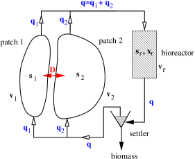
Figure 1: Modeling scheme of the treatment of two interconnected patches (definitions of the variables and parameters are given in Section 2)

In the present work, we consider that the treatment of the water resource can be split into two zones i.e. the water is extracted from the resource at two different points (instead of one), and the treated water returns to the resource (with the same flows) at two different locations. A diffusion makes connection between the zones (see Fig. 1). Such a division into two patches can represent real situations such as:

• natural environments where water tables or lagoons are connected together by a small communication path (this modeling covers also the particular case of a null diffusion when one has to treat two independent volumes),

• resource hydrodynamics that reveal influence zones for each pumping devices, depending on the locations of the extraction and return points,

• accidental pollution as an homogeneous strain diffusing into the complementary part of the resource.

The control problem consists in choosing dynamically the total flow rate $q$ and the flow distribution $q_{1}$, $q_{2}$ between the two patches, with the objective of having both of them decontaminated in minimal time. Notice that a particular strategy consists in having all the time a flow distribution entirely with one zone, which amounts to the former problem with active and dead zones mentioned above. We study here the benefit of switching dynamically the treatment to the other patch or treating simultaneously both patches. The associated minimal-time problem is significantly more complex, because there are two controls and the velocity set is non-convex (this is shown in the next Section). Indeed, it is necessary to use different techniques to address the cases of non-null diffusion between the two zones and the limiting case of null diffusion between the two zones.

The paper is organized as follows. In the next section, definitions and assumptions are presented. In Section 3, properties of the optimization problem with relaxed controls and non-null diffusion are investigated. In Section 4, the optimal control strategy for the original problem with non-null diffusion is given and proven. In Section 5, we address the particular case of null diffusion and we provide explicit bounds on the minimal-time function. Finally, we show numerical computations that illustrate the theoretical results, and give concluding remarks.

2 Definitions and preliminaries

In what follows, we denote by $\mathbb{R}$ the set of real numbers, $\mathbb{R}_{+}$ and $\mathbb{R}_{+}^{\star}$ the sets of non-negative and positive real numbers respectively. Analogously, $\mathbb{R}_{-}$ and $\mathbb{R}_{-}^{\star}$ are the sets of non-positive and negative real numbers respectively. We set also $\mathbb{R}_{+}^{2}=\mathbb{R}_{+}\times\mathbb{R}_{+}$ and $\mathbb{R}_{-}^{2}=\mathbb{R}_{-}\times\mathbb{R}_{-}$.

The time evolution of the concentrations $s_{i}$ ($i=1,2$) of pollutants in the two patches are given by the equations

$$\left\{\begin{array}[]{lll}\displaystyle\frac{ds_{1}}{dt}&=&\displaystyle\frac{q_{1}}{v_{1}}(s_{{\rm{r}}}-s_{1})+\frac{D}{v_{1}}(s_{2}-s_{1})\ ,\\[8.53581pt] \displaystyle\frac{ds_{2}}{dt}&=&\displaystyle\frac{q_{2}}{v_{2}}(s_{{\rm{r}}}-s_{2})+\frac{D}{v_{2}}(s_{1}-s_{2})\ ,\end{array}\right.$$ (1)

where the volumes $v_{i}$ ($i=1,2$) are assumed to be constant and $D$ denotes the diffusion coefficient of the pollutant between the two zones. The control variables are the flow rates $q_{i}$ of the pumps in each zone, which bring water with a low pollutant concentration $s_{{\rm{r}}}$ from the bioreactor and remove water with a pollutant concentration $s_{i}$ from each zone $i$, with the same flow rates $q_{i}$.

The concentration $s_{{\rm{r}}}$ at the output of the bioreactor is linked to the total flow rate $q=q_{1}+q_{2}$ by the usual chemostat model:

$$\left\{\begin{array}[]{lll}\displaystyle\frac{ds_{{\rm{r}}}}{dt}&=&\displaystyle-\mu(s_{{\rm{r}}})x_{{\rm{r}}}+\frac{q}{v_{{\rm{r}}}}(s_{in}-s_{{\rm{r}}})\ ,\\[8.53581pt] \displaystyle\frac{dx_{{\rm{r}}}}{dt}&=&\displaystyle\mu(s_{{\rm{r}}})x_{{\rm{r}}}-\frac{q}{v_{{\rm{r}}}}x_{{\rm{r}}}\ ,\end{array}\right.$$ (2)

where $x_{{\rm{r}}}$ is the biomass concentration, $v_{{\rm{r}}}$ is the volume of the bioreactor and $\mu(\cdot)$ is the specific growth rate of the bacteria (without a loss of generality we assume that the yield coefficient is equal to one). These equations describe the dynamics of a bacterial growth consuming a substrate that is constantly fed in a tank of constant volume (see for instance [23]). The input concentration $s_{in}$ is given here by the combination of the concentrations of the water extracted from the two zones:

$$s_{in}=\frac{q_{1}s_{1}+q_{2}s_{2}}{q_{1}+q_{2}}\ .$$ (3)

We assume that the output of the bioreactor is filtered by a settler, that we assume to be perfect, so that the water that returns to the resource is biomass free (see [9, 10] for considerations of settler modeling and conditions that ensure the stability of the desired steady-state of the settler).

The target to be reached in the minimal time is defined by a threshold $\underline{s}>0$ of the pollutant concentrations, that is

$${\cal T}=\left\{s=(s_{1},s_{2})\in\mathbb{R}_{+}^{2}\,|\,\max(s_{1},s_{2})\leq\underline{s}\right\}\ .$$ (4)

In the paper, we shall denote $t_{f}$ as the first time at which a trajectory reaches the target (when it exists).

We make the usual assumptions on the growth function $\mu(\cdot)$ in absence of inhibition.

Assumption 1

$\mu(\cdot)$ is a $C^{1}$ increasing concave function defined on $\mathbb{R}_{+}$ with $\mu(0)=0$.

Under this last assumption, we recall that under a constant $s_{in}$, the dynamics (2) admit a unique positive equilibrium $(s_{{\rm{r}}}^{\star},x_{{\rm{r}}}^{\star})$ that is globally asymptotically stable on the domain $\mathbb{R}_{+}\times\mathbb{R}_{+}^{\star}$ provided that the condition $q/v_{{\rm{r}}}\leq\mu(s_{in})$ is satisfied (see, for instance, [23]). Then, $s_{{\rm{r}}}^{\star}$ is defined as the unique solution of $\mu(s_{{\rm{r}}}^{\star})=q/v_{{\rm{r}}}$ and $x_{{\rm{r}}}^{\star}=s_{in}-s_{{\rm{r}}}^{\star}$. Consequently, considering expression (3), the controls $q_{1}$ and $q_{2}$ are chosen such that

$$q_{1}+q_{2}\leq v_{{\rm{r}}}\mu\left(\frac{q_{1}s_{1}+q_{2}s_{2}}{q_{1}+q_{2}}\right)\ .$$ (5)

We assume that the resource to be treated is very large. This amounts to considering that the bioreactor is small compared to both zones of the resource.

Assumption 2

$v_{1}$ and $v_{2}$ are large compared to $v_{{\rm{r}}}$.

Let us define $\alpha=q_{1}/q$, $r=v_{1}/(v_{1}+v_{2})$, $d=D/v_{{\rm{r}}}$, and $\epsilon=v_{{\rm{r}}}/(v_{1}+v_{2})$. Then, the coupled dynamics (1)-(2) with (3) can be written in the slow-fast form

$$\left\{\begin{array}[]{lll}\displaystyle\frac{ds_{{\rm{r}}}}{dt}&=&\displaystyle-\mu(s_{{\rm{r}}})x_{{\rm{r}}}+\frac{q}{v_{{\rm{r}}}}(\alpha s_{1}+(1-\alpha)s_{2}-s_{{\rm{r}}})\ ,\\[8.53581pt] \displaystyle\frac{dx_{{\rm{r}}}}{dt}&=&\displaystyle\mu(s_{{\rm{r}}})x_{{\rm{r}}}-\frac{q}{v_{{\rm{r}}}}x_{{\rm{r}}}\ ,\\[8.53581pt] \displaystyle\frac{ds_{1}}{dt}&=&\displaystyle\epsilon\left(\frac{\alpha}{r}\frac{q}{v_{{\rm{r}}}}(s_{{\rm{r}}}-s_{1})+\frac{d}{r}(s_{2}-s_{1})\right)\ ,\\[8.53581pt] \displaystyle\frac{ds_{2}}{dt}&=&\displaystyle\epsilon\left(\frac{1-\alpha}{1-r}\frac{q}{v_{{\rm{r}}}}(s_{{\rm{r}}}-s_{2})+\frac{d}{1-r}(s_{1}-s_{2})\right)\ .\end{array}\right.$$ (6)

Provided that the initial conditions of the variables $(s_{{\rm{r}}},x_{{\rm{r}}})$ belong to $\mathbb{R}_{+}\times\mathbb{R}_{+}^{\star}$, applying Tikonov’s Theorem (see for instance [16]), the dynamics of the slow variables $(s_{1},s_{2})$ can be approached using the reduced dynamics

$$\left\{\begin{array}[]{lllll}\displaystyle\dot{s}_{1}&=&\displaystyle\frac{ds_{1}}{d\tau}&=&\displaystyle\frac{\alpha}{r}\mu(s_{{\rm{r}}}^{\star})(s_{{\rm{r}}}^{\star}-s_{1})+\frac{d}{r}(s_{2}-s_{1})\ ,\\[8.53581pt] \displaystyle\dot{s}_{2}&=&\displaystyle\frac{ds_{2}}{d\tau}&=&\displaystyle\frac{1-\alpha}{1-r}\mu(s_{{\rm{r}}}^{\star})(s_{{\rm{r}}}^{\star}-s_{2})+\frac{d}{1-r}(s_{1}-s_{2})\end{array}\right.$$ (7)

in the time scale $\tau=\epsilon t$. In this formulation, the quasi-steady-state concentration $s_{{\rm{r}}}^{\star}$ of the bioreactor can be considered as a control variable that takes values in $[0,\alpha s_{1}+(1-\alpha)s_{2}]$, which is equivalent to choosing $q\in[0,v_{{\rm{r}}}\mu(\alpha s_{1}+(1-\alpha)s_{2})]$ when Assumption 1 is satisfied. In the following, we shall consider the optimal control for the reduced dynamics only. Nevertheless, we give some properties of the optimal feedback for the reduced dynamics when applied to the un-reduced one, in Section 4 (Remark 2) and Appendix.

Notice that the control problem can be reformulated with the controls $u=(\alpha,s_{{\rm{r}}}^{\star})$ that belong to the state-dependent control set

$$U(s)=\left\{(\alpha,s_{{\rm{r}}}^{\star})\,|\,\alpha\in[0,1],\;s_{{\rm{r}}}^{\star}\in[0,\alpha s_{1}+(1-\alpha)s_{2}]\right\}$$ (8)

equivalently to controls $q_{1}$ and $q_{2}$. In what follows, a measurable function $u(\cdot)$ such that $u(t)\in U(s(t))$ for all $t$ is called an admissible control.

Lemma 1

The domain $\mathbb{R}_{+}^{2}$ is positively invariant by the dynamics (7) for any admissible controls $u(\cdot)$, and any trajectory is bounded. Furthermore, the target ${\cal T}$ is reachable in a finite time from any initial condition in $\mathbb{R}_{+}^{2}$.

Proof. For $s_{1}=0$ and $s_{2}\geq 0$, one has $\dot{s}_{1}\geq 0$. Similarly, one has $\dot{s}_{2}\geq 0$ when $s_{1}\geq 0$ and $s_{2}=0$. By the uniqueness of the solutions of (7) for measurable controls $u(\cdot)$, we deduce that $\mathbb{R}_{+}^{2}$ is invariant. From equations (7), one can write

$$r\dot{s}_{1}+(1-r)\dot{s}_{2}=\mu(s_{{\rm{r}}}^{\star})(s_{{\rm{r}}}^{\star}-(\alpha s_{1}+(1-\alpha)s_{2}))\leq 0$$

for any admissible controls. One then deduces

$$rs_{1}(t)+(1-r)s_{2}(t)\leq M_{0}=rs_{1}(0)+(1-r)s_{2}(0),\quad\forall t\geq 0,$$

which provides the boundedness of the trajectories.

Consider the feedback strategy

$$\alpha=r\ ,\;s_{{\rm{r}}}^{\star}=\frac{rs_{1}+(1-r)s_{2}}{2},$$

and we write the dynamics of $m=rs_{1}+(1-r)s_{2}$ as follows:

$$\dot{m}=-\mu\left(\frac{m}{2}\right)\frac{m}{2}<0\ ,\forall m>0\ .$$

Then, from any initial condition in $\mathbb{R}_{+}^{2}$, the solution $m(t)$ tends to $0$ when $t$ tends to infinity. Therefore, $m(\cdot)$ reaches the set $[0,\min(r,1-r)\underline{s}]$ in a finite time, which guarantees that $s=(s_{1},s_{2})$ belongs to ${\cal T}$ at that time.  

For simplicity, we define the function

$$\beta(\sigma,s_{{\rm{r}}}^{\star})=\mu(s_{{\rm{r}}}^{\star})(\sigma-s_{{\rm{r}}}^{\star})$$ (9)

so that the dynamics (7) can be written in the more compact form

$$\dot{s}=F(s,u)+dG(s)$$ (10)

where $F(\cdot)$ and $G(\cdot)$ are defined as follows:

$$F(s,(\alpha,s_{{\rm{r}}}^{\star}))=-\left[\begin{array}[]{c}\displaystyle\frac{\alpha}{r}\beta(s_{1},s_{{\rm{r}}}^{\star})\\[5.69054pt] \displaystyle\frac{1-\alpha}{1-r}\beta(s_{2},s_{{\rm{r}}}^{\star})\end{array}\right],\quad G(s)=\left[\begin{array}[]{c}\displaystyle\frac{s_{2}-s_{1}}{r}\\[5.69054pt] \displaystyle\frac{s_{1}-s_{2}}{1-r}\end{array}\right]\ .$$

The dynamics can be equivalently expressed in terms of controls $v=(\alpha,\zeta)$ that belong to the state-independent set $V=[0,1]^{2}$ with the dynamics

$$\dot{s}=F(s,(\alpha,\zeta(\alpha s_{1}+(1-\alpha)s_{2})))+dG(s)$$ (11)

which satisfy the usual regularity conditions for applying Pontryagin’s Maximum Principle for deriving necessary optimality conditions. One can notice that the velocity set of the dynamics (11) is not everywhere convex. Consequently, one cannot guarantee a priori the existence of an optimal control $v(\cdot)$ in the set of time-measurable functions that take values in $V$ but that are among relaxed controls (see, for instance, [27, Sec. 2.7]). For convenience, we shall keep the formulation of the problem with controls $u$. Because for any $s$ the sets $\cup_{u\in U(s)}F(s,u)$ are two-dimensional connected, the corresponding convexified dynamics can be written as follows (see [19, Th. 2.29]):

$$\dot{s}=\tilde{F}(s,\tilde{u})+dG(s)$$ (12)

with

$$\tilde{F}(s,\tilde{u})=pF(s,u_{a})+(1-p)F(s,u_{b})$$ (13)

where the relaxed controls $\tilde{u}=(u_{a},u_{b},p)=(\alpha_{a},s_{{\rm{r}}a}^{\star},\alpha_{b},s_{{\rm{r}}b}^{\star},p)$ belong to the set

$$\tilde{U}(s)=U(s)^{2}\times[0,1].$$

In the next section, we show that the relaxed problem admits an optimal solution that is also a solution of the original (non-relaxed) problem.

3 Study of the relaxed problem

Throughout this section, we assume that the parameter $d$ is positive. The particular case of $d=0$ will be considered later in Section 5. Let us write the Hamiltonian of the relaxed problem

$$\begin{multlined}\tilde{H}(s,\lambda,(\alpha_{a},s_{{\rm{r}}a}^{\star},\alpha_{b},s_{{\rm{r}}b}^{\star},p))=\\ -1+p\,Q(s,\lambda,(\alpha_{a},s_{{\rm{r}}a}^{\star}))+(1-p)\,Q(s,\lambda,(\alpha_{b},s_{{\rm{r}}b}^{\star}))+d(s_{2}-s_{1})\left(\frac{\lambda_{1}}{r}-\frac{\lambda_{2}}{1-r}\right)\end{multlined}\tilde{H}(s,\lambda,(\alpha_{a},s_{{\rm{r}}a}^{\star},\alpha_{b},s_{{\rm{r}}b}^{\star},p))=\\ -1+p\,Q(s,\lambda,(\alpha_{a},s_{{\rm{r}}a}^{\star}))+(1-p)\,Q(s,\lambda,(\alpha_{b},s_{{\rm{r}}b}^{\star}))+d(s_{2}-s_{1})\left(\frac{\lambda_{1}}{r}-\frac{\lambda_{2}}{1-r}\right)$$ (14)

which is to be maximized w.r.t. $(\alpha_{a},s_{{\rm{r}}a}^{\star},\alpha_{b},s_{{\rm{r}}b}^{\star},p)\in\tilde{U}(s)$, where $\lambda=(\lambda_{1},\lambda_{2})$, and we have defined, for convenience, the function

$$Q(s,\lambda,(\alpha,s_{{\rm{r}}}^{\star}))=-\left(\alpha\frac{\lambda_{1}}{r}\beta(s_{1},s_{{\rm{r}}}^{\star})+(1-\alpha)\frac{\lambda_{2}}{1-r}\beta(s_{2},s_{{\rm{r}}}^{\star})\right)\ .$$ (15)

The adjoint equations are

$$\left\{\begin{array}[]{lll}\displaystyle\dot{\lambda}_{1}&=&\displaystyle\lambda_{1}\left(p\frac{\alpha_{a}}{r}\mu(s_{{\rm{r}}a}^{\star})+(1-p)\frac{\alpha_{b}}{r}\mu(s_{{\rm{r}}b}^{\star})+\frac{d}{r}\right)-\lambda_{2}\frac{d}{1-r}\ ,\\[8.53581pt] \displaystyle\dot{\lambda}_{2}&=&\displaystyle-\lambda_{1}\frac{d}{r}+\lambda_{2}\left(p\frac{1-\alpha_{a}}{1-r}\mu(s_{{\rm{r}}a}^{\star})+(1-p)\frac{1-\alpha_{b}}{1-r}\mu(s_{{\rm{r}}b}^{\star})+\frac{d}{1-r}\right)\ ,\end{array}\right.$$ (16)

with the following transversality conditions

$$\left\{\begin{array}[]{lll}s_{1}(t_{f})<\underline{s},\;s_{2}(t_{f})=\underline{s}&\Rightarrow&\lambda_{1}(t_{f})=0,\;\lambda_{2}(t_{f})<0\ ,\\ s_{1}(t_{f})=\underline{s},\;s_{2}(t_{f})<\underline{s}&\Rightarrow&\lambda_{1}(t_{f})<0,\;\lambda_{2}(t_{f})=0\ ,\\ s_{1}(t_{f})=\underline{s},\;s_{2}(t_{f})=\underline{s}&\Rightarrow&\lambda_{1}(t_{f})\leq 0,\;\lambda_{2}(t_{f})\leq 0\mbox{ with }\lambda(t_{f})\neq 0\ .\end{array}\right.$$ (17)

As usual, a triple $(s(\cdot),\lambda(\cdot),\tilde{u}^{\star}(\cdot))$ satisfying (12), (16), (17), and

$$\tilde{H}(s(t),\lambda(t),\tilde{u}^{\star}(t))=\max_{\tilde{u}\in\tilde{U}(s(t))}\tilde{H}(s(t),\lambda(t),\tilde{u})$$ (18)

is called an admissible extremal.

Lemma 2

Along any admissible extremal, one has $\lambda_{i}(t)<0$ ($i=1,2$) for any $t<t_{f}$.

Proof. If one writes the adjoint equations (16) as $\dot{\lambda}_{i}=\phi_{i}(t,\lambda_{1},\lambda_{2})$ ($i=1,2$), one can notice that the partial derivatives $\partial_{j}\phi_{i}$ ($i\neq j$) are non-positive. From the theory of monotone dynamical systems (see for instance [22]), the dynamics (16) is thus competitive or, equivalently, cooperative in backward time. As the transversality conditions (17) gives $\lambda_{i}(t_{f})\leq 0$ ($i=1,2$), we deduce by the property of monotone dynamics that one should have $\lambda_{i}(t)\leq 0$ ($i=1,2$) for any $t\leq t_{f}$. Moreover, $\lambda=0$ is an equilibrium of (16) and $\lambda(t_{f})$ has to be different from $0$ at any time $t\leq t_{f}$. Then, $\lambda_{i}(t)$ ($i=1,2$) cannot be simultaneously equal to zero. If there exists $t<t_{f}$ and $i\in\{1,2\}$ such that $\lambda_{i}(t)=0$, then one should have $\lambda_{j}(t)<0$ for $j\neq i$. However, $d>0$ implies $\dot{\lambda}_{i}(t)>0$, thus obtaining a contradiction with $\lambda_{i}\leq 0$ for any time.  

For the following, we consider the function

$$\gamma(\sigma)=\max_{s_{{\rm{r}}}^{\star}\geq 0}\beta(\sigma,s_{{\rm{r}}}^{\star}),\quad\sigma>0\ ,$$ (19)

which satisfies the following property:

Lemma 3

Under Assumption 1, for any $\sigma>0$, there exists a unique $\hat{s}_{{\rm{r}}}^{\star}(\sigma)\in(0,\sigma)$ that realizes the maximum in (19). Furthermore, the function $\gamma(\cdot)$ is differentiable and increasing with

$$\gamma^{\prime}(\sigma)=\mu(\hat{s}_{{\rm{r}}}^{\star}(\sigma))\ .$$ (20)

Proof. Consider the function $\varphi:(\sigma,w)\in\mathbb{R}_{+}\times[0,1]\mapsto\beta(\sigma,w\sigma)$ and the partial function $\varphi_{\sigma}:w\in[0,1]\mapsto\varphi(\sigma,w)$ for fixed $\sigma>0$. Notice that $\varphi_{\sigma}(0)=\varphi_{\sigma}(1)=0$ and that $\varphi_{\sigma}(w)>0$ for $w\in(0,1)$. Simple calculation gives $\varphi_{\sigma}^{\prime\prime}(w)=\mu^{\prime\prime}(w\sigma)(1-w)\sigma^{3}-2\mu^{\prime}(w\sigma)\sigma^{2}$, which is negative. Therefore, $\varphi_{\sigma}(\cdot)$ is a strictly concave function on $[0,1]$ and consequently admits a unique maximum $w^{\star}_{\sigma}$ on $[0,1]$. We conclude that $w^{\star}_{\sigma}$ belongs to $(0,1)$ or, equivalently, that the maximum of $s_{{\rm{r}}}^{\star}\mapsto\beta(\sigma,s_{{\rm{r}}}^{\star})$ is realized for a unique $\hat{s}_{{\rm{r}}}^{\star}(\sigma)=w^{\star}_{\sigma}\sigma$ in $(0,\sigma)$.

Furthermore, one has $\varphi_{\sigma}^{\prime}(w)=\sigma\mu^{\prime}(w\sigma)(\sigma-w\sigma)-\sigma\mu(w\sigma)$, and the necessary optimality condition $\varphi_{\sigma}^{\prime}(w^{\star}_{\sigma})=0$ gives the equality

$$\mu(\hat{s}_{{\rm{r}}}^{\star}(\sigma))=\mu^{\prime}(\hat{s}_{{\rm{r}}}^{\star}(\sigma))(\sigma-\hat{s}_{{\rm{r}}}^{\star}(\sigma))\ .$$ (21)

Simple calculation shows that for each $w\in[0,1]$, the function $\sigma\mapsto\varphi(\sigma,w)$ is convex. Because the maximizer $w_{\sigma}^{\star}$ of $\varphi_{\sigma}(\cdot)$ is unique for any $\sigma$, one can apply the rules of differentiability of pointwise maxima (see, for instance, [7, Chap. 2.8]), which state that the function $\gamma(\sigma)=\max_{w\in[0,1]}\varphi(\sigma,w)$ is differentiable with

$$\gamma^{\prime}(\sigma)=\frac{\partial\varphi}{\partial\sigma}(\sigma,w^{\star}_{\sigma}\sigma)=w_{\sigma}^{\star}\mu^{\prime}(w_{\sigma}^{\star}\sigma)(\sigma-w_{\sigma}^{\star}\sigma)+\mu(w_{\sigma}^{\star}\sigma)(1-w_{\sigma}^{\star})\ .$$

Equation (21) provides the simpler expression (20), which shows that $\gamma(\cdot)$ is increasing.  

We now consider the variable

$$\eta=\frac{-\lambda_{1}}{r}\,\gamma(s_{1})-\frac{-\lambda_{2}}{1-r}\,\gamma(s_{2})$$ (22)

which will play the role of a switching function. Notice that this is not the usual switching function of problems with linear dynamics w.r.t. a scalar control because our problem has two controls $\alpha$ and $s_{{\rm{r}}}^{\star}$ that cannot be separated, and the second control acts non-linearly in the dynamics.

Lemma 4

For fixed $(s,\lambda)\in\mathbb{R}_{+}^{2}\times\mathbb{R}_{-}^{2}$, the pairs $u^{\star}=(\alpha,s_{r}^{\star})\in U(s)$ that maximize the function $Q(s,\lambda,\cdot)$ are the following:

1. when $\eta>0$: $u^{\star}=(1,\hat{s}_{{\rm{r}}}^{\star}(s_{1}))$,

2. when $\eta<0$: $u^{\star}=(0,\hat{s}_{{\rm{r}}}^{\star}(s_{2}))$,

3. when $\eta=0$ and $s_{1}=s_{2}$: $u^{\star}\in[0,1]\times\{\hat{s}_{{\rm{r}}}^{\star}\}$ where $\hat{s}_{{\rm{r}}}^{\star}=\hat{s}_{{\rm{r}}}^{\star}(s_{1})=\hat{s}_{{\rm{r}}}^{\star}(s_{2})$,

4. when $\eta=0$ and $s_{1}\neq s_{2}$: $u^{\star}=(1,\hat{s}_{{\rm{r}}}^{\star}(s_{1}))$ or $u^{\star}=(0,\hat{s}_{{\rm{r}}}^{\star}(s_{2}))$.

Proof. When $\eta>0$, one can write, using Lemma 3 and $\lambda_{1},\lambda_{2}<0$,

$$\begin{array}[]{lll}Q(s,\lambda,(1,\hat{s}_{{\rm{r}}}^{\star}(s_{1})))&=&\displaystyle\frac{-\lambda_{1}}{r}\gamma(s_{1})\\ &>&\displaystyle\alpha\frac{-\lambda_{1}}{r}\gamma(s_{1})+(1-\alpha)\frac{-\lambda_{2}}{1-r}\gamma(s_{2})\ ,\;\forall\alpha\in[0,1)\\ &\geq&\displaystyle\alpha\frac{-\lambda_{1}}{r}\beta(s_{1},s_{{\rm{r}}}^{\star})+(1-\alpha)\frac{-\lambda_{2}}{1-r}\beta(s_{2},s_{{\rm{r}}}^{\star})\ ,\;\forall\alpha\in[0,1),\;\forall s_{{\rm{r}}}^{\star}\in[0,\alpha s_{1}+(1-\alpha)s_{2}],\\ &\geq&\displaystyle Q(s,\lambda,(\alpha,s_{{\rm{r}}}^{\star}))\ ,\;\forall\alpha\in[0,1),\;\forall s_{{\rm{r}}}^{\star}\in[0,\alpha s_{1}+(1-\alpha)s_{2}],\end{array}$$

and for $\alpha=1$, one has $Q(s,\lambda,(1,\hat{s}_{{\rm{r}}}^{\star}(s_{1})))>Q(s,\lambda,(1,s_{{\rm{r}}}^{\star}))\ ,\forall s_{{\rm{r}}}^{\star}\neq\hat{s}_{{\rm{r}}}^{\star}(s_{1})$. Therefore, the maximum of $Q(s,\lambda,\cdot)$ is reached for the unique pair $(\alpha,s_{{\rm{r}}}^{\star})=(1,s_{{\rm{r}}}^{\star}(s_{1}))$.

Similarly, when $\eta<0$, one can show that the unique maximum is $(\alpha,s_{{\rm{r}}}^{\star})=(0,s_{{\rm{r}}}^{\star}(s_{2}))$.

When $\eta=0$, one has

$$\frac{-\lambda_{1}}{r}\gamma(s_{1})=\frac{-\lambda_{2}}{1-r}\gamma(s_{2})>Q(s,\lambda,(\alpha,s_{{\rm{r}}}^{\star}))\ ,\forall\alpha\in[0,1]\ ,\forall s_{{\rm{r}}}^{\star}\notin\{\hat{s}_{{\rm{r}}}^{\star}(s_{1}),\hat{s}_{{\rm{r}}}^{\star}(s_{2})\}.$$

If $s_{1}=s_{2}$, one necessarily has $\lambda_{1}/r=\lambda_{2}/(1-r)\neq 0$, and thus,

$$Q(s,\lambda,(\alpha,s_{{\rm{r}}}^{\star}))=\frac{-\lambda_{1}}{r}\beta(s_{1},s_{{\rm{r}}}^{\star})<\frac{-\lambda_{1}}{r}\gamma(s_{1})=Q(s,\lambda,(\alpha,\hat{s}_{{\rm{r}}}^{\star}(s_{1})))\ ,\forall s_{1}^{\star}\neq\hat{s}_{{\rm{r}}}^{\star}(s_{1}),$$

for any $\alpha\in[0,1]$. The optimal $s_{{\rm{r}}}^{\star}$ is necessarily equal to $\hat{s}_{{\rm{r}}}^{\star}(s_{1})=\hat{s}_{{\rm{r}}}^{\star}(s_{2})$.

If $s_{1}\neq s_{2}$, one has $\tilde{s}_{{\rm{r}}}^{\star}(s_{1})\neq\hat{s}_{{\rm{r}}}^{\star}(s_{2})$, and consequently, using Lemma 3 and the fact that $\lambda_{1}$ and $\lambda_{2}$ are both negative,

$$Q(s,\lambda,(\alpha,\hat{s}_{{\rm{r}}}^{\star}(s_{1})))=\alpha\frac{-\lambda_{1}}{r}\gamma(s_{1})+(1-\alpha)\frac{-\lambda_{2}}{1-r}\beta(s_{2},\hat{s}_{{\rm{r}}}^{\star}(s_{1}))<\frac{-\lambda_{1}}{r}\gamma(s_{1})\ ,\forall\alpha\in[0,1)$$

$$Q(s,\lambda,(\alpha,\hat{s}_{{\rm{r}}}^{\star}(s_{2})))=\alpha\frac{-\lambda_{1}}{r}\beta(s_{1},\hat{s}_{{\rm{r}}}^{\star}(s_{2}))+(1-\alpha)\frac{-\lambda_{2}}{1-r}\gamma(s_{2})<\frac{-\lambda_{2}}{1-r}\gamma(s_{2})\ ,\forall\alpha\in(0,1]$$

Then, $(\alpha,s_{{\rm{r}}}^{\star})=(1,\hat{s}_{{\rm{r}}}^{\star}(s_{1}))$ and $(\alpha,s_{{\rm{r}}}^{\star})=(0,\hat{s}_{{\rm{r}}}^{\star}(s_{2}))$ are the only two pairs that maximize $Q(s,\lambda,\cdot)$.  

Proposition 1

At almost any time, an optimal control $\tilde{u}^{\star}$ of the relaxed problem satisfies the following property:

1. when $\eta\neq 0$ or $s_{1}=s_{2}$, one has $\tilde{F}(s,\tilde{u}^{\star})=F(s,u^{\star})$, where $u^{\star}$ is given by Lemma 4 i.-ii.-iii.

2. when $\eta=0$ and $s_{1}\neq s_{2}$, one has

   $$\begin{multlined}\tilde{u}^{\star}\in\{(1,\hat{s}_{{\rm{r}}}^{\star}(s_{1})),(0,\hat{s}_{{\rm{r}}}^{\star}(s_{2}))\}\times U(s)\times\{1\}\;\cup\;U(s)\times\{(1,\hat{s}_{{\rm{r}}}^{\star}(s_{1})),(0,\hat{s}_{{\rm{r}}}^{\star}(s_{2}))\}\times\{0\}\\ \;\cup\;\{(1,\hat{s}_{{\rm{r}}}^{\star}(s_{1}),0,\hat{s}_{{\rm{r}}}^{\star}(s_{2}))\}\times[0,1]\;\cup\;\{(0,\hat{s}_{{\rm{r}}}^{\star}(s_{2}),1,\hat{s}_{{\rm{r}}}^{\star}(s_{1}))\}\times[0,1].\end{multlined}\tilde{u}^{\star}\in\{(1,\hat{s}_{{\rm{r}}}^{\star}(s_{1})),(0,\hat{s}_{{\rm{r}}}^{\star}(s_{2}))\}\times U(s)\times\{1\}\;\cup\;U(s)\times\{(1,\hat{s}_{{\rm{r}}}^{\star}(s_{1})),(0,\hat{s}_{{\rm{r}}}^{\star}(s_{2}))\}\times\{0\}\\ \;\cup\;\{(1,\hat{s}_{{\rm{r}}}^{\star}(s_{1}),0,\hat{s}_{{\rm{r}}}^{\star}(s_{2}))\}\times[0,1]\;\cup\;\{(0,\hat{s}_{{\rm{r}}}^{\star}(s_{2}),1,\hat{s}_{{\rm{r}}}^{\star}(s_{1}))\}\times[0,1].$$ (23)

Proof. According to Pontryagin’s Maximum Principle, an optimal control $\tilde{u}=(u_{a},u_{b},p)$ has to maximize for a.e. time the Hamiltonian $\tilde{H}$ given in (14) or, equivalently, the quantity

$$(u_{a},u_{b},p)\longmapsto\tilde{Q}(s,\lambda,(u_{a},u_{b},p))=pQ(s,\lambda,u_{a})+(1-p)Q(s,\lambda,u_{b})$$

where $\lambda_{1}$ and $\lambda_{2}$ are negative (from Lemma 2). Let us consider the maximization of the function $Q(s,\lambda,\cdot)$ characterized by Lemma 4.

In cases i and ii, the function $Q(s,\lambda,\cdot)$ admits a unique maximizer $u^{\star}$. Thus, $\tilde{Q}(s,\lambda,\cdot)$ is maximized for $u_{a}=u^{\star}$ with $p=1$ independent of $u_{b}$ (or, symmetrically, for $u_{b}=u^{\star}$ with $p=0$ independent of $u_{a}$) or for $u_{a}=u_{b}=u^{\star}$ independent of $p\in[0,1]$. In any case, one has $\tilde{F}(s,\tilde{u}^{\star})=F(s,u^{\star})$.

In case iii, the function $Q(s,\lambda,\cdot)$ is maximized for a unique value of $s_{{\rm{r}}}^{\star}=\hat{s}_{r}^{\star}(s_{1})=\hat{s}_{r}^{\star}(s_{2})$ independent of $\alpha$. Thus, $\tilde{Q}(s,\lambda,\cdot)$ is maximized when $s_{{\rm{r}}a}^{\star}$ is equal to this value with $p=1$ independent of $u_{b}$ (and, symmetrically, when $s_{{\rm{r}}b}^{\star}$ is equal to this value with $p=0$ independent of $u_{a}$) or when both $s_{{\rm{r}}a}^{\star}$ and $s_{{\rm{r}}b}^{\star}$ are equal to this value independent of $\alpha_{a}$, $\alpha_{b}$ and $p$. In any case, one has $\tilde{F}(s,\tilde{u}^{\star})=F(s,u^{\star})$, where $u^{\star}\in[0,1]\times\{s_{{\rm{r}}}^{\star}\}$.

In case iv, the function $Q(s,\lambda,\cdot)$ admits two possible maximizers. Thus, $\tilde{Q}(s,\lambda,\cdot)$ is maximized when $u_{a}$ is equal to one of these maximizers with $p=1$ independent of $u_{b}$, when, symmetrically, $u_{b}$ is equal to one of these maximizers with $p=0$ independent of $u_{a}$, or when $u_{a}$ and $u_{b}$ are equal to the two different maximizers independent of $p$. All these cases appear in the set-membership (23).  

Remark 1

In case 2 of Proposition 1, a relaxed control $\tilde{u}^{\star}$ with $p\in(0,1)$ can be approximated by a high-frequency switching between non-relaxed controls $u=(1,\hat{s}_{{\rm{r}}}^{\star}(s_{1}))$ and $u=(0,\hat{s}_{{\rm{r}}}^{\star}(s_{2}))$ (see the “chattering control” in [6]). In practice, such a high-frequency switching between the two pumps is not desired.

The following Lemma will be crucial later at several places.

Lemma 5

Along any extremal trajectory, one has at almost any time

$$\dot{\eta}=d\left(\frac{\gamma(s_{1})}{r}+\frac{\gamma(s_{2})}{1-r}\right)\left(\frac{\lambda_{2}}{1-r}-\frac{\lambda_{1}}{r}\right)+d\left(\frac{\lambda_{1}}{r^{2}}\mu(\hat{s}_{{\rm{r}}}^{\star}(s_{1}))+\frac{\lambda_{2}}{(1-r)^{2}}\mu(\hat{s}_{{\rm{r}}}^{\star}(s_{2}))\right)(s_{1}-s_{2})\ .$$ (24)

Proof. Let us write the time derivatives of the products $\lambda_{1}\gamma(s_{1})$ and $\lambda_{2}\gamma(s_{2})$ that appear in the expression of the function $\eta$ using expressions (12), (16) and (20):

$$\frac{d}{dt}\left[\lambda_{1}\gamma(s_{1})\right]=\frac{\lambda_{1}}{r}\delta_{1}+d\gamma(s_{1})\left(\frac{\lambda_{1}}{r}-\frac{\lambda_{2}}{1-r}\right)+d\frac{\lambda_{1}}{r}\mu(\hat{s}_{{\rm{r}}}^{\star}(s_{1}))(s_{2}-s_{1})$$

where we put

$$\delta_{1}=p\alpha_{a}\left[\mu(s_{{\rm{r}}a}^{\star})\gamma(s_{1})-\mu(\hat{s}_{{\rm{r}}}^{\star}(s_{1}))\beta(s_{1},s_{{\rm{r}}a}^{\star})\right]+(1-p)\alpha_{b}\left[\mu(s_{{\rm{r}}b}^{\star})\gamma(s_{1})-\mu(\hat{s}_{{\rm{r}}}^{\star}(s_{1}))\beta(s_{1},s_{{\rm{r}}b}^{\star})\right].$$

One can easily check that for any optimal control $\tilde{u}^{\star}$ given by Proposition 1, one has $\delta_{1}=0$. Similarly, one can write

$$\frac{d}{dt}\left[\lambda_{2}\gamma(s_{2})\right]=\frac{\lambda_{2}}{1-r}\delta_{2}+d\gamma(s_{2})\left(\frac{\lambda_{2}}{1-r}-\frac{\lambda_{1}}{r}\right)+d\frac{\lambda_{2}}{1-r}\mu(\hat{s}_{{\rm{r}}}^{\star}(s_{2}))(s_{1}-s_{2})$$

where

$$\delta_{2}=p(1-\alpha_{a})\left[\mu(s_{{\rm{r}}a}^{\star})\gamma(s_{2})-\mu(\hat{s}_{{\rm{r}}}^{\star}(s_{2}))\beta(s_{2},s_{{\rm{r}}a}^{\star})\right]+(1-p)(1-\alpha_{b})\left[\mu(s_{{\rm{r}}b}^{\star})\gamma(s_{2})-\mu(\hat{s}_{{\rm{r}}}^{\star}(s_{2}))\beta(s_{2},s_{{\rm{r}}b}^{\star})\right],$$

with $\delta_{2}=0$ for any optimal control $\tilde{u}^{\star}$ given by Proposition 1.

Then, one obtains the equality (24).  

We now prove that the non-relaxed problem admits an optimal solution that is also optimal for the relaxed problem.

Proposition 2

The optimal trajectories for the problem with the convexified dynamics (12) are admissible optimal trajectories for the original dynamics (10). Furthermore, the optimal control $u^{\star}(\cdot)$ satisfies the following property

$$s_{1}(t)\neq s_{2}(t)\Longrightarrow u^{\star}(t)=(1,\hat{s}_{{\rm{r}}}^{\star}(s_{1}))\mbox{ or }u^{\star}(t)=(0,\hat{s}_{{\rm{r}}}^{\star}(s_{2})),\quad\mbox{for a.e. }t\in[0,t_{f}]\ .$$

Proof. We will prove that the set of times whereby the optimal relaxed strategy generates a velocity that belongs to the convexified velocity set but not to the original velocity set has Lebesgue measure zero. For this, consider $s_{1}>s_{2}$ and $\eta=0$. Because $\gamma(\cdot)$ is increasing (see Lemma 3), $\gamma(s_{1})>\gamma(s_{2})$. Additionally, $\eta=0$ implies that $\lambda_{1}/r>\lambda_{2}/(1-r)$. From equation (24) of Lemma 5, we deduce the inequality $\dot{\eta}<0$ (where $\lambda_{1}$ and $\lambda_{2}$ are negative by Lemma 2). Similarly, to consider $s_{2}>s_{1}$ and $\eta=0$ implies that $\dot{\eta}>0$. We conclude that case 2 of Proposition 1 can only occur at times in a set of null measure, from which the statement follows.

Now, because the optimal strategy of the convexified problem is (at almost any time) an admissible extremal for the original problem, and because the optimal time of the convexified problem is less than or equal to the optimal time of the original problem, the original problem has a solution, and it is characterized by point 1 of Proposition 1.

The last statement of the proposition follows from point 1 of Proposition 1.  

4 Synthesis of the optimal strategy

According to Proposition 2, we can now consider optimal trajectories of the original (non-relaxed) problem, knowing that the optimal strategy is “bang-bang” except on a possible singular arc that belongs to the diagonal set $\Delta:=\{s\in\mathbb{R}_{+}^{2}\mbox{ s.t. }s_{1}=s_{2}\}$.

Proposition 3

For $d>0$, the following feedback control drives any initial state in $\mathbb{R}_{+}^{2}\setminus{\cal T}$ to the target ${\cal T}$ in minimal time:

$$u^{\star}[s]=\left|\begin{array}[]{ll}(1,\hat{s}_{{\rm{r}}}^{\star}(s_{1}))&\mbox{when }s_{1}>s_{2}\ ,\\ (r,\hat{s}_{{\rm{r}}}^{\star}(s_{1}))=(r,\hat{s}_{{\rm{r}}}^{\star}(s_{2}))&\mbox{when }s_{1}=s_{2}\ ,\\ (0,\hat{s}_{{\rm{r}}}^{\star}(s_{2}))&\mbox{when }s_{1}<s_{2}\ .\end{array}\right.$$ (25)

Proof. From Pontryagin’s Maximum Principle, a necessary optimality condition for an admissible trajectory is the existence of a solution to the adjoint system

$$\left\{\begin{array}[]{lll}\displaystyle\dot{\lambda}_{1}&=&\displaystyle\lambda_{1}\frac{\alpha}{r}\mu(s_{{\rm{r}}}^{\star})+d\left(\frac{\lambda_{1}}{r}-\frac{\lambda_{2}}{1-r}\right)\ ,\\[8.53581pt] \displaystyle\dot{\lambda}_{2}&=&\displaystyle\lambda_{2}\frac{1-\alpha}{1-r}\mu(s_{{\rm{r}}}^{\star})+d\left(\frac{\lambda_{2}}{1-r}-\frac{\lambda_{1}}{r}\right)\ ,\end{array}\right.$$ (26)

with the transversality conditions (17) and where $u^{\star}=(\alpha,s_{{\rm{r}}}^{\star})$ maximizes the Hamiltonian

$$H(s,\lambda,u)=-1+Q(s,\lambda,u)+d(s_{2}-s_{1})\left(\frac{\lambda_{1}}{r}-\frac{\lambda_{2}}{1-r}\right)$$

w.r.t. $u$.

Consider the set

$$I_{-}=\left\{(s,\eta)\in(\mathbb{R}_{+}^{2}\setminus{\cal T})\times\mathbb{R}\mbox{ s.t. }s_{1}>s_{2}\mbox{ and }\eta<0\right\}\ .$$

From expression (24), one obtains the property

$$s_{1}>s_{2}\mbox{ and }\eta<0\;\Rightarrow\;\dot{\eta}<0$$

using the facts that $\lambda_{i}$ ($i=1,2$) are negative (Lemma 2) and that $\gamma(\cdot)$ is increasing (Lemma 3). When $\eta<0$, one has $u^{\star}=(0,\hat{s}_{{\rm{r}}}^{\star}(s_{2}))$ from Lemma 4, and it is possible to write

$$\dot{s}_{1}-\dot{s}_{2}=-\frac{d}{r(1-r)}(s_{1}-s_{2})+\frac{\gamma(s_{2})}{1-r},$$

which shows that $s_{1}-s_{2}$ remains positive for any future time. Thus, the set $I_{-}$ is positively invariant by the dynamics defined by systems (7) and 26). We deduce that the existence of a time $t<t_{f}$ such that $(s(t),\eta(t))\in I_{-}$ implies $(s(t_{f}),\eta(t_{f}))\in I_{-}$, and from the transversality condition (17), one obtains $\lambda_{1}(t_{f})<\lambda_{2}(t_{f})=0$. Then, one should have $\eta(t_{f})=-\lambda_{1}(t_{f})\gamma(s_{1}(t_{f}))/r>0$, thus obtaining a contradiction. Similarly, one can show that the set

$$I_{+}=\left\{(s,\eta)\in(\mathbb{R}_{+}^{2}\setminus{\cal T})\times\mathbb{R}\mbox{ s.t. }s_{1}<s_{2}\mbox{ and }\eta>0\right\}$$

is positively invariant and that the transversality condition implies that $(s,\eta)$ never belongs to $I_{+}$ along an optimal trajectory. Because $\Delta$ is the only possible locus of a singular arc, we can form a conclusion about the optimality of (25) outside $\Delta$.

Now, consider the function

$$L(s)=\frac{1}{2}(s_{1}-s_{2})^{2}$$

and write its time derivative along an admissible trajectory $s(\cdot)$ as follows:

$$\dot{L}=\langle\nabla L,\dot{s}\rangle=\left(-\frac{\alpha}{r}\beta(s_{1},s_{{\rm{r}}}^{\star})+\frac{1-\alpha}{1-r}\beta(s_{2},s_{{\rm{r}}}^{\star})\right)(s_{1}-s_{2})-\frac{2d}{r(1-r)}L\ .$$

Along an optimal trajectory, one has

$$\dot{L}+\frac{2d}{r(1-r)}L=\left|\begin{array}[]{ll}\displaystyle-\frac{\gamma(s_{1})}{r}(s_{1}-s_{2})&\mbox{when }s_{1}>s_{2},\\[5.69054pt] \displaystyle\,\,\,\frac{\gamma(s_{2})}{1-r}(s_{1}-s_{2})&\mbox{when }s_{1}<s_{2},\end{array}\right.$$

and deduces that the inequality $\dot{L}+\frac{2d}{r(1-r)}L\leq 0$ is satisfied. Consequently, the set $\Delta\subset L^{-1}(0)$ is positively invariant by the optimal dynamics. On $\Delta$, the maximization of $Q(s,\lambda,\cdot)$ gives the unique $s_{{\rm{r}}}^{*}=\hat{s}_{{\rm{r}}}^{\star}(s_{1})=\hat{s}_{{\rm{r}}}^{\star}(s_{2})$ because $\lambda_{1}$, $\lambda_{2}$ are both negative (see Lemmas 2, 3 and 4). Finally, the only (non-relaxed) control that leaves $\Delta$ invariant is such that $\alpha=r$.  

Remark 2

The feedback (25) has been proved to be optimal for the reduced dynamics (7). In the Appendix, we prove that this feedback drives the state of the un-reduced dynamics (6) to the target in finite time, whatever is $\epsilon>0$. In Section 6, we show on numerical simulations how the time to reach the target is close from the minimal time of the reduced dynamics when $\epsilon$ is small.

5 Study of the minimal-time function

Define the function

$$T(\sigma)=\max(0,\overline{T}(\sigma))\quad\mbox{with}\quad\overline{T}(\sigma)=\int_{\underline{s}}^{\sigma}\frac{d\xi}{\gamma(\xi)},\quad\sigma>0\ .$$

Lemma 6

$T(\cdot)$ is strictly concave on $[\underline{s},+\infty)$.

Proof. Lemma 3 allows one to claim that $\overline{T}(\cdot)$ is twice differentiable for any $\sigma>0$ and that one has

$$\overline{T}^{\prime\prime}(\sigma)=-\frac{\gamma^{\prime}(\sigma)}{\gamma(\sigma)^{2}}<0\ ,\quad\forall\sigma>0\ .$$

The function $\overline{T}(\cdot)$ is strictly concave on $\mathbb{R}_{+}$, and because $T(\cdot)$ coincides with $\overline{T}(\cdot)$ on $[\underline{s},+\infty)$, we conclude that $T(\cdot)$ is strictly concave on this interval.  

Let us denote the minimal-time function by $V_{d}(\cdot)$, indexed by the value of the parameter $d$:

$$V_{d}(x)=\inf_{u(\cdot)}\left\{t>0\,|\,s(x,u,d,t)\in{\cal T}\right\},$$

where $s(x,u,d,\cdot)$ denotes the solution of (10) with the initial condition $s(0)=x=(x_{1},x_{2})$, the admissible control $u(\cdot)$ and the parameter value $d$. Lemma 1 ensures that these functions are well defined on $\mathbb{R}_{+}^{2}$.

Proposition 4

The value functions $V_{d}(\cdot)$ satisfy the following properties.

1. For any $d\geq 0$, $V_{d}(\cdot)$ is Lipschitz continuous on $\mathbb{R}_{+}^{2}$.

2. For $d=0$, one has $V_{0}(x)=rT(x_{1})+(1-r)T(x_{2})$ for any $x\in\mathbb{R}_{+}^{2}$, and the feedback (25) is optimal for both relaxed and non-relaxed problems.

Proof. On the boundary $\partial^{+}{\cal T}$ of the target that lies in the interior of the (positively) invariant domain $\mathbb{R}_{+}^{2}$, the set $N(\cdot)$ of unitary external normals is

$$N(s)=\left|\begin{array}[]{ll}\left\{\left(\begin{array}[]{c}0\\ 1\end{array}\right)\right\}&\mbox{when }s_{1}<\underline{s}\mbox{ and }s_{2}=\underline{s},\\[11.38109pt] \left\{\left(\begin{array}[]{c}\cos\theta\\ \sin\theta\end{array}\right)\right\}_{\theta\in[0,\pi/2]}&\mbox{when }s_{1}=s_{2}=\underline{s},\\[11.38109pt] \left\{\left(\begin{array}[]{c}1\\ 0\end{array}\right)\right\}&\mbox{when }s_{1}=\underline{s}\mbox{ and }s_{2}<\underline{s}\ .\end{array}\right.$$

At any $s\in\partial^{+}{\cal T}$, one has

$$\inf_{u\in U(s)}\inf_{\nu\in N(s)}\langle F(s,u)+dG(s),\nu\rangle\leq\inf_{u\in U(s)}\inf_{\nu\in N(s)}\langle F(s,u),\nu\rangle=-\gamma(\underline{s})<0\ .$$

Furthermore, the maps

$$s\mapsto F(s,u)+dG(s)$$

are Lipschitz continuous w.r.t. $s\in\mathbb{R}_{+}^{2}$ uniformly in $u$. According to [4, Sect 1. and 4, Chap. IV], the target satisfies then the small time locally controllable property, and the value functions $V_{d}(\cdot)$ are Lipschitz continuous on $\mathbb{R}_{+}^{2}$.

When $d=0$, the feedback (25) provides the following dynamics

$$\dot{s}=\left|\begin{array}[]{rl}-\frac{1}{r}\left[\begin{array}[]{c}\gamma(s_{1})\\ 0\end{array}\right]&\mbox{when }s_{1}>\max(s_{2},\underline{s})\ ,\\[11.38109pt] -\left[\begin{array}[]{c}\gamma(s_{1})\\ \gamma(s_{2})\end{array}\right]&\mbox{when }s_{1}=s_{2}>\underline{s}\ ,\\[11.38109pt] -\frac{1}{1-r}\left[\begin{array}[]{c}0\\ \gamma(s_{2})\end{array}\right]&\mbox{when }s_{2}>\max(s_{1},\underline{s})\ ,\end{array}\right.$$

and one can explicitly calculate the time to go to the target for any initial condition $x\in\mathbb{R}_{+}^{2}$, which we denote as $W_{0}(x)$:

$$W_{0}(x)=\left|\begin{array}[]{ll}\displaystyle-r\int_{x_{1}}^{\max(x_{2},\underline{s})}\frac{ds_{1}}{\gamma(s_{1})}-\int_{\max(x_{2},\underline{s})}^{\underline{s}}\frac{ds_{1}}{\gamma(s_{1})}&\mbox{when }x_{1}\geq x_{2}\ ,\\[11.38109pt] \displaystyle-(1-r)\int_{x_{2}}^{\max(x_{1},\underline{s})}\frac{ds_{2}}{\gamma(s_{2})}-\int_{\max(x_{1},\underline{s})}^{\underline{s}}\frac{ds_{2}}{\gamma(s_{2})}&\mbox{when }x_{1}\leq x_{2}\ .\end{array}\right.$$

One can check that $W_{0}$ is Lipschitz continuous and that it can be written as $W_{0}(x)=rT(x_{1})+(1-r)T(x_{2})$. We now show that $W_{0}$ is a viscosity solution of the Hamilton-Jacobi-Bellman equation associated to the relaxed problem

$${\cal H}(x,\nabla W_{0}(x))=-1+\max_{(u_{a},u_{b},p)\in\tilde{U}(x)}pQ(x,-\nabla W_{0}(x),u_{a})+(1-p)Q(x,-\nabla W_{0}(x),u_{b})=0,\quad x\notin{\cal T},$$ (27)

(where $Q$ is defined in (15)) with the boundary condition

$$W_{0}(x)=0,\quad x\in{\cal T}\ .$$ (28)

Consider the $C^{1}$ functions

$$\overline{W}_{0,1}(x)=r\overline{T}(x_{1})\quad,\quad\overline{W}_{0,2}(x)=(1-r)\overline{T}(x_{2})\quad\mbox{and}\quad\overline{W}_{0}(x)=\overline{W}_{0,1}(x)+\overline{W}_{0,2}(x)$$

defined on $\mathbb{R}_{+}^{2}$. One has

$$\nabla\overline{W}_{0,1}(x)=\left[\begin{array}[]{c}\displaystyle\frac{r}{\gamma(x_{1})}\\[11.38109pt] 0\end{array}\right]\quad\mbox{and}\quad\nabla\overline{W}_{0,2}(x)=\left[\begin{array}[]{c}0\\[11.38109pt] \displaystyle\frac{1-r}{\gamma(x_{2})}\end{array}\right]$$

which are non-negative vectors. One can then use Lemma 4 to obtain the property

$${\cal H}(x,\nabla\overline{W}_{0,1}(x))={\cal H}(x,\nabla\overline{W}_{0,2}(x))={\cal H}(x,\nabla\overline{W}_{0}(x))=0,\quad x\in\mathbb{R}_{+}^{2}\ ,$$

which shows that $\overline{W}_{0,1}$, $\overline{W}_{0,2}$ and $\overline{W}_{0}$ are solutions of (27) in the classical sense.

At $x\notin{\cal T}$ with $x_{i}\neq\underline{s}$ ($i=1,2$), $W_{0}$ is $C^{1}$ and locally coincides with $\overline{W}_{0}$. Then, it satisfies equation (27) in the classical sense.

At $x\notin{\cal T}$ with $x_{1}=\underline{s}$ or $x_{2}=\underline{s}$, $W_{0}$ is not differentiable but locally coincides with $\max(\overline{W}_{0},\overline{W}_{0,2})$ or $\max(\overline{W}_{0},\overline{W}_{0,1})$. From the properties of viscosity solutions (see, for instance, [4, Prop 2.1, Chap. II]), one must simply check that $W_{0}$ is a super-solution of (27). At such points, the Fréchet sub-differential of $W_{0}$ is

$$\partial^{-}W_{0}(x)=\left|\begin{array}[]{ll}\displaystyle\left[0,\frac{r}{\gamma(\underline{s})}\right]\times\left\{\frac{1-r}{\gamma(x_{2})}\right\}&\mbox{when }x_{1}=\underline{s}\ ,\\[11.38109pt] \displaystyle\left\{\frac{r}{\gamma(x_{1})}\right\}\times\left[0,\frac{1-r}{\gamma(\underline{s})}\right]&\mbox{when }x_{2}=\underline{s}\ .\end{array}\right.$$

Because any sub-gradient $\delta^{-}\in\partial^{-}W_{0}(x)$ is a non-negative vector, one can again use Lemma 4 and obtain

$${\cal H}(x,\delta^{-})=0,\quad\forall\delta^{-}\in\partial^{-}W_{0}(x)\ ,$$

which proves that $W_{0}$ is a viscosity solution of (27). Moreover, $W_{0}$ satisfies the boundary condition (28). Finally, we use the characterization of the minimal-time function as the unique viscosity solution of (27) in the class of Lipschitz continuous functions with boundary conditions (28) (see [4, Th. 2.6, Chap IV]) to conclude that $W_{0}$ is the value function of the relaxed problem. Because the time $W_{0}(x)$ to reach the target from an initial condition $x\notin{\cal T}$ is obtained with the non-relaxed control (25), we also deduce that $V_{0}$ and $W_{0}$ are equal.  

Remark 3

In the case $d=0$, the control given by (25) is optimal but not the unique solution of the problem. Indeed, in Proposition 4, we proved that $V_{0}(\cdot)$ is the unique viscosity solution to equation (27), where one of the possible maximizers of the Hamiltonian given in (27) is given by (25), but on the set $(\underline{s},\infty)^{2}\setminus\Delta$ there are more choices for $u$; for instance,

$$u^{\star}[s]=\left|\begin{array}[]{ll}(1,\hat{s}_{{\rm{r}}}^{\star}(s_{1}))&\mbox{when }s_{2}\leq\underline{s}<s_{1}\ ,\\ (0,\hat{s}_{{\rm{r}}}^{\star}(s_{2}))&\mbox{when }s_{1}>s_{2}>\underline{s}\ ,\\ (r,\hat{s}_{{\rm{r}}}^{\star}(s_{1}))=(r,\hat{s}_{{\rm{r}}}^{\star}(s_{2}))&\mbox{when }s_{1}=s_{2}\ ,\\ (1,\hat{s}_{{\rm{r}}}^{\star}(s_{1}))&\mbox{when }\underline{s}<s_{1}<s_{2}\ ,\\ (0,\hat{s}_{{\rm{r}}}^{\star}(s_{2}))&\mbox{when }s_{1}\leq\underline{s}<s_{2}\end{array}\right.$$

satisfies (27).

Proposition 5

The functions $V_{d}(\cdot)$ satisfy the following properties:

1. $V_{d}(x)=T(x_{1})=T(x_{2})$ for any $x\in\Delta$ and $d\geq 0$,

2. $V_{\infty}(x)=\lim_{d\to+\infty}V_{d}(x)=T(rx_{1}+(1-r)x_{2})$ for any $x\in\mathbb{R}_{+}^{2}$, and

3. $d\mapsto V_{d}(x)$ is increasing for any $x\in(\underline{s},+\infty)^{2}\setminus\Delta$.

Proof. Consider an initial condition $x$ in $\Delta\setminus{\cal T}$. The optimal synthesis given in Proposition 3 shows that the set $\Delta$ is invariant by the optimal flow and that the dynamics on $\Delta$ are

$$\dot{s}_{i}=-\gamma(s_{i}),\quad i=1,2$$

independent of $d$. We then conclude that $V_{d}(x)=T(x_{i})$ for $i=1,2$.

Consider $d>0$ and $x\notin\Delta\cup{\cal T}$. Denote for simplicity $s(\cdot)$ as the solution $s(x,u^{\star},d,\cdot)$ with the feedback control $u^{\star}$ given in Proposition 3, and $t_{f}=V_{d}(x)$. Define $t_{\Delta}$ as the first time $t$ such that $s(t)\in\Delta$ (here, we allow the solution $s(\cdot)$ to possibly enter the target ${\cal T}$ before reaching $\Delta$).

From equation (10) with control (25), one can easily check that the following inequalities are satisfied

$$\begin{array}[]{l}x_{1}>x_{2}\Rightarrow x_{1}>s_{1}(t)\geq s_{2}(t)>x_{2},\quad\forall t\in[0,t_{\Delta}]\ ,\\[5.69054pt] x_{1}<x_{2}\Rightarrow x_{1}<s_{1}(t)\leq s_{2}(t)<x_{2},\quad\forall t\in[0,t_{\Delta}]\ .\end{array}$$

Then, because the function $\gamma(\cdot)$ is increasing (Lemma 3), one can write, if the state $s$ has not yet reached $\Delta$,

$$-\frac{d}{r(1-r)}|s_{1}-s_{2}|-M_{+}\leq\frac{d}{dt}|s_{1}-s_{2}|\leq-\frac{d}{r(1-r)}|s_{1}-s_{2}|-M_{-}$$ (29)

with $M_{-}=\min(\gamma(x_{2})/r,\gamma(x_{1})/(1-r))$ and $M_{+}=\max(\gamma(x_{1})/r,\gamma(x_{2})/(1-r))$. Then, we obtain an upper bound on the time $t_{\Delta}$

$$t_{\Delta}\leq\frac{r(1-r)}{d}\log\left(1+d\frac{|x_{1}-x_{2}|}{M_{-}r(1-r)}\right)$$ (30)

which tends to zero when $d$ tends to infinity. From (29), we can also write

$$|x_{1}-x_{2}|-M_{+}t_{\Delta}\leq\frac{d}{r(1-r)}\int_{0}^{t_{\Delta}}|s_{2}(\tau)-s_{1}(\tau)|d\tau\leq|x_{1}-x_{2}|-M_{-}t_{\Delta}$$

and finally, one obtains from (10) the following bounds on $s_{i}(t_{\Delta})$ ($i=1,2$):

$$rx_{1}+(1-r)x_{2}-\max(r,(1-r))M_{+}t_{\Delta}\leq s_{i}(t_{\Delta})\leq rx_{1}+(1-r)x_{2}-\min(r,(1-r))M_{-}t_{\Delta}\ .$$ (31)

Therefore, $s_{1}(t_{\Delta})=s_{2}(t_{\Delta})$ converges to $rx_{1}+(1-r)x_{2}$ when $d$ tends to $+\infty$. Furthermore, one has

$$\begin{array}[]{ll}t_{f}=t_{\Delta}+T(s(t_{\Delta}))&\mbox{when }s(t_{\Delta})\notin{\cal T}\ ,\\ t_{f}<t_{\Delta}&\mbox{when }s(t_{\Delta})\in{\cal T}\ .\end{array}$$

Because $t_{\Delta}\to 0$ and because $T(\cdot)$ is continuous with $T(rx_{1}+(1-r)x_{2})=0$ when $rx_{1}+(1-r)x_{2}\leq\underline{s}$, we obtain the convergence

$$V_{\infty}(x)=\lim_{d\to+\infty}V_{d}(x)=T(rx_{1}+(1-r)x_{2})\ .$$

Now, consider the domain ${\cal D}_{+}=\{s\in\mathbb{R}_{+}^{2}\,|\,s_{1}\geq s_{2}>\underline{s}\}$, and let us show that any trajectory of the optimal flow leaves ${\cal D}_{+}$ at $(\underline{s},\underline{s})$ with the help of this simple argumentation on the boundaries of the domain:

$$\begin{array}[]{l}\displaystyle s_{2}=\underline{s}\;\Rightarrow\;\dot{s}_{2}=\frac{d}{1-r}(s_{1}-\underline{s})\geq 0\ ,\\[8.53581pt] \displaystyle s_{1}=s_{2}\;\Rightarrow\;\dot{s}_{1}=\dot{s}_{2}\ .\end{array}$$

It is convenient to consider the variable $\tilde{s}=rs_{1}+(1-r)s_{2}$, whose optimal dynamics in ${\cal D}_{+}$ are simply

$$\dot{\tilde{s}}(t)=-\gamma(s_{1}(t))\ ,\quad t\in[0,t_{f}]\ .$$ (32)

Because $\tilde{s}(\cdot)$ is strictly decreasing with time, an optimal trajectory in ${\cal D}_{+}$ can be parameterized by the fictitious time

$$\tau(t)=rx_{1}+(1-r)x_{2}-\tilde{s}(t)\ ,\quad t\in[0,t_{f}]$$ (33)

(where $x$ is an initial condition in ${\cal D}_{+}$). The variable $s_{1}(\cdot)$ is then a solution of the scalar non-autonomous dynamics

$$\frac{ds_{1}}{d\tau}=f_{d}(\tau,s_{1})=\left|\begin{array}[]{ll}\displaystyle-\frac{1}{r}-d\frac{s_{1}+\tau-(rx_{1}+(1-r)x_{2})}{r(1-r)\gamma(s_{1})}&\mbox{when }s_{1}+\tau>rx_{1}+(1-r)x_{2}\ ,\\[8.53581pt] -1&\mbox{when }s_{1}+\tau=rx_{1}+(1-r)x_{2}\ ,\end{array}\right.$$

with the terminal fictitious time

$$\tau_{f}=rx_{1}+(1-r)x_{2}-\underline{s}\ .$$

Notice that $\tau_{f}$ is independent of $d$. One then deduces the inequalities

$$d_{1}>d_{2}\mbox{ and }s_{1}+\tau>rx_{1}+(1-r)x_{2}\Longrightarrow f_{d_{1}}(\tau,s_{1})<f_{d_{2}}(\tau,s_{1})$$

and thus,

$$d_{1}>d_{2}\mbox{ and }x\in{\cal D}_{+}\setminus\Delta\Longrightarrow s_{1}(x,u^{\star},d_{1},\tau)<s_{1}(x,u^{\star},d_{2},\tau)\ ,\;\forall\tau\in[0,\tau_{f}]\ .$$ (34)

Finally, from equations (32) and (33), the time to reach the target can be expressed as

$$t_{f}=\int_{0}^{\tau_{f}}\frac{d\tau}{\gamma(s_{1}(\tau))}\ .$$ (35)

Because the function $\gamma(\cdot)$ is increasing and because $\tau_{f}$ is independent of $d$, one can conclude from (34) and (35) that

$$d_{1}>d_{2}\mbox{ and }x\in{\cal D}_{+}\setminus\Delta\Longrightarrow V_{d_{1}}(x)>V_{d_{2}}(x)\ .$$

The case of initial conditions in ${\cal D}_{-}\setminus\Delta$, with ${\cal D}_{-}=\{s\in\mathbb{R}_{+}^{2}\,|\,s_{2}\geq s_{1}>\underline{s}\}$, is symmetric.  

Remark 4

The tightness $V_{\infty}-V_{0}$ of the bounds on the value function $V_{d}$ on $(\underline{s},+\infty)^{2}\setminus\Delta$ is related to the concavity of the function $T(\cdot)$ on $(\underline{s},+\infty)$ (the less the concavity $\max_{\sigma\in[\underline{s},+\infty)}|\overline{T}^{\prime\prime}(\sigma)|$ is, the tighter the bounds are).

The bounds $V_{0}\leq V_{d}<V_{\infty}$ that are satisfied on the set $(\underline{s},+\infty)^{2}\setminus\Delta$ are not necessarily satisfied outside this set: for $x$ outside the target but such that $rx_{1}+(1-r)x_{2}<\underline{s}$, one has $V_{\infty}(x)=0$ and $V_{0}(x)>0$. Therefore, we conclude that a large diffusion negatively impacts the time to treat the resource when both zones are initially polluted; however, when one of the two zones is initially under the pollution threshold, a large diffusion could positively impact the duration of the treatment.

6 Numerical illustrations

We consider the Monod (or Michaelis-Menten) growth function, which is quite popular in bio-processes and which satisfies Assumption 1:

$$\mu(s)=\mu_{\max}\frac{s}{K_{s}+s},$$

with the parameters $\mu_{\max}=1[h^{-1}]$ and $K_{s}=1[gL^{-1}]$. The corresponding function $\gamma(\cdot)$ is depicted in Fig. 2. The threshold that defines the target has been chosen as $\underline{s}=1[gL^{-1}]$.

Figure 2: Graphs of $\mu(\cdot)$ and corresponding $\gamma(\cdot)$.

Several optimal trajectories in the phase portrait are drawn in Fig. 3 for small and large values of the parameter $d$.

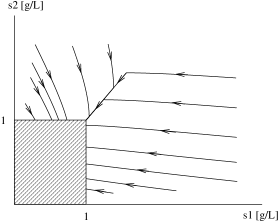
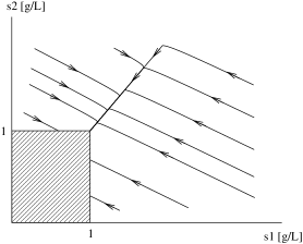
Figure 3: Optimal paths for $d=0.1[h^{-1}]$ (left) and $d=10[h^{-1}]$ (right) with $r=0.3$.

Finally, level sets of the value functions $V_{0}$ and $V_{\infty}$ are represented in Fig. 4.

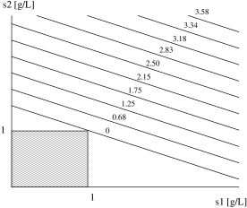
Figure 4: Level sets (in hours) of $V_{0}$ (left) and $V_{\infty}$ (right) for $r=0.3$.

One can make the following observations concerning the influence of the diffusion on the treatment duration, that we consider to be valuable from a practical viewpoint.

• When pollution is homogeneous, the best is to maintain it homogeneous, and the treatment time is then independent of the diffusion.

• A high diffusion is favorable for having fast treatments when initial concentrations are strongly different for the two zones. Typically, when the pollutant concentration is below the threshold in one patch, a high diffusion can reduce significantly the treatment time compared to a small diffusion.

• When initial concentrations in the two patches are close, a small diffusion leads to faster treatment than a large diffusion.

For various initial condition $s(0)$, we have also performed numerical comparisons of the minimal time $V_{d}(s(0))$ given by the feedback strategy (25) against two other non-optimal control strategies:

1. the best constant control that gives the smallest time $T^{\star}_{cst}$ to reach the target among constant controls,

2. the optimal one-pump feedback strategy obtained in the former work [14]. This last control strategy considers that only one patch can be treated (that we called the “active zone”). The problem amounts then to consider the same dynamics (7) but one seeks the feedback $s_{{\rm{r}}}^{\star}(\cdot)$ that gives the minimal time $T^{\star}_{one}$ when $\alpha$ is imposed to be constantly equal to $1$ (or $0$ depending which patch is treated). In [14], it has been proved that the feedback $s_{1}\mapsto\hat{s}_{{\rm{r}}}^{\star}(s_{1})$ is optimal.

	$\mathbf{V}_{d}$		$\mathbf{T_{cst}^{\star}}$		$\mathbf{T_{one}^{\star}}$
	$d=0.1$	$d=10$	$d=0.1$	$d=10$	$d=0.1$	$d=10$
$s(0)=(1.5,0)$	0.42	0.01	0.42	0.01	0.42	0.01
Increase:			(+ 1.45 %)	(+ 0.00 %)	(+ 0.00 %)	(+ 0.00 %)
$s(0)=(3,0)$	1.01	0.06	1.05	0.06	1.01	0.06
Increase:			(+ 3.90 %)	(+ 0.85 %)	(+ 0.00 %)	(+ 0.00 %)
$s(0)=(4,0.5)$	1.33	2.17	1.39	2.23	1.37	2.21
Increase:			(+ 4.68 %)	(+ 2.62 %)	(+ 2.73 %)	(+ 1.55 %)
$s(0)=(4,1.5)$	3.20	3.65	3.67	3.75	8.27	3.72
Increase:			(+ 14.76 %)	(+ 2.58 %)	(+ 158.27 %)	(+ 1.91 %)
$s(0)=(4,4)$	5.45	5.45	5.74	5.71	18.25	5.53
Increase:			(+ 5.43 %)	(+ 4.90 %)	(+ 235.01 %)	(+ 1.59 %)

	$\mathbf{V}_{d}$		$\mathbf{T_{cst}^{\star}}$		$\mathbf{T_{one}^{\star}}$
	$d=0.1$	$d=10$	$d=0.1$	$d=10$	$d=0.1$	$d=10$
$s(0)=(1.5,0)$	25.95	34.12	38.65	38.81	34.03	34.14
Increase:			(+ 48.93 %)	(+ 13.74 %)	(+ 31.14 %)	(+ 0.05 %)
$s(0)=(3,0)$	32.91	39.91	50.08	50.12	45.89	40.15
Increase:			(+ 52.18 %)	(+ 25.58 %)	(+ 39.45 %)	(+ 0.60 %)
$s(0)=(4,0.5)$	41.08	42.86	58.65	58.02	61.51	42.94
Increase:			(+ 42.77 %)	(+ 35.37 %)	(+ 49.74 %)	(+ 0.1 %)
$s(0)=(4,1.5)$	43.69	44.37	63.59	63.28	70.81	44.49
Increase:			(+ 45.57 %)	(+ 42.61 %)	(+ 62.08 %)	(+ 0.27 %)
$s(0)=(4,4)$	45.94	45.94	71.67	71.04	81.58	46.17
Increase:			(+ 56.02 %)	(+ 54.64 %)	(+ 77.60 %)	(+ 0.51 %)

Table 1: Time comparisons (in hours) for $r=0.3$ and target value $\underline{s}=1$ (top), $0.1$ (bottom) $[gL^{-1}]$ (initial condition $s(0)$ and diffusion parameter $d$ are given in $gL^{-1}$ and $h^{-1}$, respectively).

The results presented in Table 1 show first that the benefit of using the optimal feedback strategy over the other strategies increases with the level of initial pollution. The simulations also demonstrate the gain of using two pumps instead of one: for large concentrations of pollutant at initial time, one can see on the tables that a constant two-pumps strategy can be even better that the optimal feedback strategy restricted to the use of one pump only. This kind of situations typically occurs when diffusion is low and the time required by the optimal strategy for using simultaneously the two pumps is large compared to the overall duration. This is particularly noticeable when the initial pollution is homogeneous and the use of two pumps allows to maintain the levels of concentrations equal in both patches. We conclude that, for small diffusion, treating only one patch without the possibility to allocate the treatment in both patches could be quite penalizing. Figure 5 illustrates the time history of the two feedback controllers.

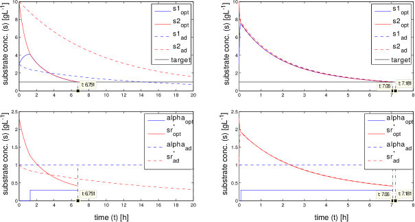
Figure 5: Trajectories and controls generated by the two-pumps and one-pump optimal feedback, for $r=0.3$, $\underline{s}=1[gL^{-1}]$ and $s(0)=(3,10)[gL^{-1}]$. On the left $d=0.1[h^{-1}]$, and on the right $d=10[h^{-1}]$.

Furthermore, the Table 1 illustrates the effect of diffusion on the treatment times. One can first notice that the relative effect of the diffusion parameter $d$ on the optimal time $V_{d}$ is decreasing with the threshold $\underline{s}$. This can be explained by the fact that the proportion of the time spent on the set $s_{1}=s_{2}$, that is independent of the parameter $d$, is larger when one begins further away from the target. One can also see that the differences between strategies decrease when the diffusion increases. Intuitively, a high diffusion makes the resource behave quickly close to a perfectly mixed resource with one patch, leading consequently to less benefit of using more than one pump. Nevertheless, one can see that considering feedback controls remain quite efficient compared to constant ones when initial pollution is high.

Finally, we illustrate on Fig. 6 the effect of approximating the original dynamics (6) by the reduced one (7), when applying the feedback (25).

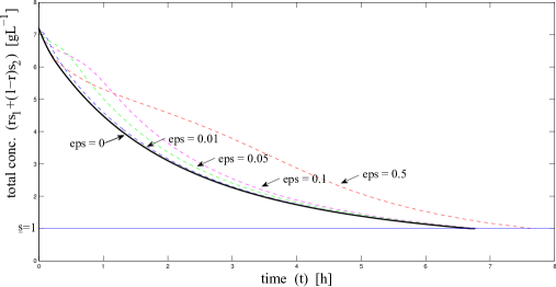
Figure 6: Total pollutant concentration in the resource of the full dynamics (6) with the strategy (25), for different values of $\epsilon$.

As proven in the Appendix, the feedback (25) drives the state to the target in finite time for any $\epsilon>0$.

7 Conclusion

In this work, we have shown that although the velocity set of the control problem is not convex, there exists an optimal solution with ordinary controls that is also optimal among relaxed controls. The optimal strategy consists in the most rapid approach to the homogenized concentration of pollutant in both patches. For the particular case of null diffusion, the most rapid approach path is not the unique solution of the problem. This optimal state-feedback has some interesting features for the practitioners and controllers:

1. it does not require knowledge of the diffusion parameter $D$ to be implemented, and

2. if the ratio $r$ of the volumes of the two patches is not known, the optimal trajectory can be approximated by a regularization of the bang-bang control about the neighborhood of the set $s_{1}=s_{2}$ that keeps the trajectory in this neighborhood.

Furthermore, is has been shown in simulations that the benefit of using two pumps instead of one can be significant when the diffusion is low. We have also proposed explicit bounds on the minimal-time function, characterizing the extreme cases $d=0$ and $d=+\infty$. We have shown that a large diffusion rate increases the treatment time when the pollution concentration is above the desired threshold in both zones, while in contrast, it can be beneficial when the concentration in one of the two zones is below the desired threshold. This remarkable feature could serve practitioners in the choice of pump positioning in an originally clean water resource that is suddenly affected by a local pollution. Such an investigation could be the matter of future work.

Appendix

Proposition 6

For any $\epsilon>0$, the feedback strategy (25) applied to the full dynamics (6) with $x_{{\rm{r}}}(0)>0$ drives the state to the target in finite time.

Proof.

Without any loss of generality, we assume that $s_{1}(0)\geq s_{2}(0)$ (the proof is similar when $s_{1}(0)\leq s_{2}(0)$).

If $s_{1}(0)>s_{2}(0)$, we prove that $s_{1}=s_{2}$ is reached in finite time. If not one, one should have $s_{1}(t)>s_{2}(t)$ with $s_{1}(t)\geq\underline{s}$ for any $t>0$. This implies to have $\alpha^{\star}(t)=1$ and $s_{{\rm{r}}}^{\star}(t)=\hat{s}_{{\rm{r}}}^{\star}(s_{1}(t))$ at any time $t>0$ and one has from equations (6):

$$r\dot{s}_{1}+(1-r)\dot{s}_{2}+\epsilon\dot{s}_{{\rm{r}}}+\epsilon\dot{x}_{{\rm{r}}}=-\epsilon\mu(s_{{\rm{r}}}^{\star})x_{{\rm{r}}}<0\ ,$$

which implies that the trajectories are bounded. For any $\sigma\geq\underline{s}$, $\hat{s}_{{\rm{r}}}^{\star}(\sigma)$ being the unique maximizer of the function $\beta(\sigma,\cdot)$, one has

$$\sigma-\hat{s}_{{\rm{r}}}^{\star}(\sigma)=\frac{\mu(\hat{s}_{{\rm{r}}}^{\star}(\sigma))}{\mu^{\prime}(\hat{s}_{{\rm{r}}}^{\star}(\sigma))}\ .$$

The function $\mu(\cdot)$ being increasing and concave, one obtains the inequality

$$\sigma-\hat{s}_{{\rm{r}}}^{\star}(\sigma)\geq\eta:=\frac{\mu(\hat{s}_{{\rm{r}}}^{\star}(\underline{s}))}{\mu^{\prime}(\hat{s}_{{\rm{r}}}^{\star}(\underline{s}))}>0\,,\quad\forall\sigma\geq\underline{s}\ .$$

Furthermore, one can write

$$r\dot{s}_{1}+\epsilon\dot{s}_{{\rm{r}}}=-d\epsilon(s_{1}-s_{2})-\mu(s_{{\rm{r}}})x_{{\rm{r}}}<0\ .$$

Thus $rs_{1}+\epsilon s_{{\rm{r}}}$ is decreasing and has a limit when $t$ tends to $+\infty$. Since the trajectories are bounded, $r\dot{s}_{1}+\epsilon\dot{s}_{{\rm{r}}}$ is uniformly continuous, and we conclude by Barbalat’s Lemma (see for instance [16]) that $r\dot{s}_{1}+\epsilon\dot{s}_{{\rm{r}}}$ converges to $0$, which implies that the positive quantities $s_{1}-s_{2}$ and $\mu(s_{{\rm{r}}})x_{{\rm{r}}}$ have to converge also to $0$. Notice that $s_{{\rm{r}}}=0$ implies $\dot{s}_{{\rm{r}}}=\mu(s_{{\rm{r}}}^{\star})s_{1}>\mu(\hat{s}_{{\rm{r}}}^{\star}(\underline{s}))\underline{s}>0$. So $s_{{\rm{r}}}$ cannot tend to $0$ and $x_{{\rm{r}}}$ has necessarily to converge to $0$. Write now the dynamics

$$\frac{d}{dt}(s_{1}-s_{{\rm{r}}})=-\left(1+\frac{\epsilon}{r}\right)\mu(s_{{\rm{r}}}^{\star})(s_{1}-s_{{\rm{r}}})-d\frac{\epsilon}{r}(s_{1}-s_{2})-\mu(s_{{\rm{r}}})x_{{\rm{r}}}\ ,$$

where $\mu(s_{{\rm{r}}}^{\star})>\mu(\hat{s}_{{\rm{r}}}^{\star}(\underline{s}))>0$ and $d\frac{\epsilon}{r}(s_{1}-s_{2})-\mu(s_{{\rm{r}}})x_{{\rm{r}}}$ tends to $0$. Thus, there exists a time $T>0$ large enough such that

$$s_{{\rm{r}}}(t)>s_{1}(t)-\eta\geq s_{{\rm{r}}}^{\star}(t)\ ,\quad\forall t>T\ ,$$

which implies to have $\mu(s_{{\rm{r}}})-\mu(s_{{\rm{r}}}^{\star})>0$ for large $t$, thus a contradiction with the convergence of $x_{{\rm{r}}}$ to $0$.

Clearly the feedback (25) leaves the set $\{s_{1}=s_{2}\}$ invariant. Denote for simplicity $s_{l}=s_{1}=s_{2}$, and write

$$\dot{s}_{l}+\epsilon\dot{s}_{{\rm{r}}}+\epsilon\dot{x}_{{\rm{r}}}=-\epsilon\mu(s_{{\rm{r}}}^{\star})x_{{\rm{r}}}<0\ .$$

Trajectories are thus bounded, and by Barbalat’s Lemma one obtains that $\mu(s_{{\rm{r}}}^{\star})x_{{\rm{r}}}$ tends to $0$. We prove now that $s_{l}$ has to reach $\underline{s}$ in finite time. If not, $\mu(s_{{\rm{r}}}^{\star}(t))>\mu(\underline{s})$ for any time and $x_{{\rm{r}}}$ tends to zero. Write the dynamics

$$\frac{d}{dt}(s_{l}-s_{{\rm{r}}})=-(1+\epsilon)\mu(s_{{\rm{r}}}^{\star})(s_{l}-s_{{\rm{r}}})+\mu(s_{{\rm{r}}})x_{{\rm{r}}}\ .$$

As before, we deduce that there exits a time $T^{\prime}>0$ such that

$$s_{{\rm{r}}}(t)>s_{l}(t)-\eta\geq s_{{\rm{r}}}^{\star}(t)\,,\quad\forall t>T^{\prime}\ ,$$

leading to a contradiction with the convergence of $x_{{\rm{r}}}$ to $0$.

References

- [1] D’Ans, G., Gottlieb, D. and Kokotovic, P. Optimal control of bacterial growth. Automatica 8, 729–736 (1972).
- [2] D’Ans, G., Kokotovic, P. and Gottlieb, D. Time-optimal control for a model of bacterial growth. J. Optim. Theory Appl. 7, 61–69 (1971).
- [3] Banga, J., Balsa-Canto, E., Moles, C. and Alonso, A. Dynamic optimization of bioreactors: a review. Proceedings of the Indian Academy of Sciences, 69, 257–265, (2003).
- [4] Bardi, M. and Capuzzo-Dolcetta, I. Optimal Control and Viscosity Solutions of Hamilton-Jacobi-Bellman Equations, Springer (1997).
- [5] Bayen T., Rapaport A. and Sebbah M. Minimal time of the two tanks gradostat model under a cascade inputs constraint, SIAM J. Optim. Control, 52(4), 2568–2594 (2014).
- [6] Borisov, V. and Zelikin, M. Theory of chattering control with applications to astronautics, robotics, economics, and engineering, Birkhäuser (1994).
- [7] Clarke, F. Optimization and Nonsmooth Analysis, Society for Industrial and Applied Mathematics (1987).
- [8] Crab, R., Avnimelech, Y., Defoirdt, T., Bossier, P. and Verstraete, W. Nitrogen removal techniques in aquaculture for a sustainable production, Aquaculture, 270 (1-4) 1–14 (2007)
- [9] Diehl, F. and Farås, S. A reduced-order ODE-PDE model for the activated sludge process in wastewater treatment: Classification and stability of steady states, math. Models Meth. Appl. Sci, 23 (3) 369–404 (2013).
- [10] Diehl, F. and Farås, S. Control of an ideal activated sludge procss in wastewater treatment via an ODE-PDE model. J. Process Control, 23 359–381 (2013).
- [11] Eding, E.H., Kamstra, A., Verreth, J.A.J., Huisman, E.A. and Klapwijk, A. Design and operation of nitrifying trickling filters in recirculating aquaculture: A review, Aquacultural Engineering, 34 (3) 234–260 (2006)
- [12] Gajardo, P., Harmand, J. and Ramírez C., H. and Rapaport, A. Minimal time bioremediation of natural water resources, Automatica 47 (8), 1764–1769 (2011).
- [13] Gajardo, P., Ramírez, H. and Rapaport, A. Minimal time sequential batch reactors with bounded and impulse controls for one or more species. SIAM Journal on Control and Optimization, 47(6) 2827–2856, ( 2008).
- [14] Gajardo, P., Ramírez C., H. Rapaport, A. and Riquelme, V. Bioremediation of Natural Water Resources via Optimal Control Techniques. In: Rubem P Mondaini. (ed): BIOMAT 2011, 178–190. BIOMAT consortium, Rio de Janeiro (2012).
- [15] Kittisupakorn, P. and Hussain, M. Comparison of optimisation based control techniques for the control of a CSTR. International Journal of Computer Applications in Technology, 13(3–5), 178–184 (2000).
- [16] Khalil, H. Nonlinear Systems, Third Ed. Prentice hall (2001).
- [17] Moreno, J. Optimal time control of bioreactors for the wastewater treatment. Optimal Control Appl. Methods, 20 (3), 145–164 (1999).
- [18] Piedrahita, R.H. Reducing the potential environmental impact of tank aquaculture effluents through intensification and recirculation, Aquaculture, 226 (1-4) 35–44 (2003)
- [19] Rockafellar T. and Wets R. Variational Analysis, Springer, Berlin (1998).
- [20] Smets, I., Claes, J., November, E., Bastin, G. and Van Impe, J. Optimal adaptive control of (bio)chemical reactors: past, present and future. Journal of Process Control, 14, 795–805 (2004).
- [21] Smets I. and Van Impe, I. Optimal control of (bio-)chemical reactors: generic properties of time and space dependent optimization. Mathematics and Computers in Simulation, 60(6) 475–486 (2002).
- [22] Smith, H. Monotone Dynamical Systems. American Mathematical Society, 1995.
- [23] Smith, H. and Waltman, P. The theory of the chemostat. Cambridge University Press, Cambridge (1995).
- [24] Soukkou, A., Khellaf, A., Leulmi, S. and Boudeghdegh., K. Optimal control of a CSTR process. Braz. J. Chem. Eng, 25(4), 799–812 (2008).
- [25] Srinivasan, B., Palanki, S. and Bonvin, D. Dynamic Optimization of Batch Processes: I. characterization of the Nominal Solution. Comput. Chem. Engng., 27(1) 1–26 (2003).
- [26] Van Impe, J. and Bastin, G. Optimal adaptive control of biotechnological processes, 401–436. Kluwer Academic Publishers (1998).
- [27] Vinter, R. Optimal Control. Birkhäuser, London (2000).