A backward dual representation for the quantile hedging of Bermudan options

Abstract

Within a Markovian complete financial market, we consider the problem of hedging a Bermudan option with a given probability. Using stochastic target and duality arguments, we derive a backward algorithm for the Fenchel transform of the pricing function. This algorithm is similar to the usual American backward induction, except that it requires two additional Fenchel transformations at each exercise date. We provide numerical illustrations.

Keywords: stochastic target problems, quantile hedging, Bermudan options.

AMS 2010 Subject Classification Primary, 91G20, 91G60 ; Secondary, 60J60, 49L20.

1 Introduction

We study the problem of hedging a claim of Bermudan style with a given probability $p$. More precisely, we want to characterize the minimal initial value $v(\cdot,p)$ of an hedging portfolio for which we can find a financial strategy such that, with a probability $p$, it remains above the exercise value of the Bermudan option at any possible exercise date.

This problem is referred to quantile hedging, and it was popularized by Föllmer et al. [12, 13] . For claims of European type, they explained how the so-called quantile hedging price can be computed explicitly when the market is complete, by using duality arguments or the Neyman-Pearson lemma. A similar question was studied in Bouchard et al. [6] but in a Markovian setting. They showed that, even in incomplete markets and for general loss functions, one can characterize the pricing function as the solution of a non-linear parabolic second order differential equation, by using tools developed in the context of stochastic target problems by Soner and Touzi [17]-[18]. When the market is complete, they also observed that taking a Legendre-Fenchel transform in the equation reduces the computation of the price to the resolution of a linear parabolic second order differential equation, which can be solved explicitly by using the Feynman-Kac formula.

As far as super-hedging is concerned, the pricing of a Bermudan option reduces to a backward sequence of pricing problems for European claims. It is therefore natural to ask whether a similar result holds for the quantile hedging price, and whether one can extend the closed-form solutions of [12] and [6] to Bermudan options.

This paper answers to the positive. Namely, we provide a backward induction algorithm for the Fenchel transform $w$ of the quantile hedging price $v(\cdot,p)$, with respect to the parameter $p$ which prescribes the probability of hedging, see (2.27) and Theorem 2.1. The algorithm (2.27) is in a sense very similar to the one used for the pricing of Bermudan options. It is however written on the Fenchel transform $w$, rather than $v$, and it involves two additional Fenchel transformations at each exercise date.

To derive this, we first build on the original idea of [6] which consists in increasing the state space in order to reduce to a stochastic target problem of American type, as studied in Bouchard and Vu [8]. We then follow a very different route. Instead of appealing to stochastic target technics, we derive from this formulation a first dynamic programming algorithm for $v$, see Proposition 2.3, which relates to a series of optimal control of martingale problems. This dynamic programming principle suggests a backward algorithm for the computation of the Fenchel transform. It is defined in (2.27). We analyze it in details in Section 3.2. The main difficulty consists in controlling the propagation of the differentiability and growth properties of the corresponding value function, backward in time. Then, as in [6, 12], a martingale representation argument allows us to show, by backward induction, that the algorithm in (2.27) and Proposition 2.3 provides the Fenchel transform of one another.

Before concluding this introduction, we would like to point out that a similar problem has been studied recently by Jiao et al. [14] in the form of general lookback-style contraints. They provide an alternative formulation in terms of an optimal control of martingale problems. This has to be compared with [5] and our Proposition 2.3. No Markovian structure is required, but they do not provide an explicit scheme as we do. Moreover, the smoothness conditions they impose on their loss functions are not satisfied in the quantile hedging case. They also study the case of several constraints in expectation set (independently) at the different exercise times, which is close to the P&L matching problems of Bouchard and Vu [7].

Finally, in this paper, we focus on the quantile hedging problem for sake of simplicity. It is an archetype of an irregular loss function, and it should be clear that a similar analysis can be carried out for a wide class of (more regular) loss functions. Also note that to obtain the dual algorithm, we only use probabilistic arguments which opens the door to the study of more general non-Markovian settings.

Notations: Let $d$ be a positive integer. Any vector $x$ of $\mathbb{R}^{d}$ is seen as a column vector. Its norm and transpose are denoted by $|x|$ and $x^{\top}$. We set $\mathbb{M}^{d}:=\mathbb{R}^{d\times d}$ and denote by $M^{\top}$ the transpose of $M\in\mathbb{M}^{d}$, while ${\rm Tr}\left[M\right]$ is its trace. For ease of notations, we set ${\mathcal{O}}_{\!+}^{d}:=(0,\infty)^{d}$.

We fix a finite time horizon $T>0$. Let $\psi:(t,x,p)\in[0,T]\times{\mathcal{O}}_{\!+}^{d}\times\mathbb{R}\mapsto\psi(t,x,p)$. If it is smooth enough, we denote by $\partial_{t}\psi$ and $\partial_{p}\psi$ its derivative with respect $t$ and $p$, and by $\partial_{x}\psi$ its Jacobian matrix with respect to $x$, as a column vector. The Hessian with respect to $x$ is $\partial^{2}_{xx}\psi$, $\partial^{2}_{pp}\psi$ is the second order derivative with respect to $p$, and $\partial^{2}_{xp}\psi$ is the vector of cross second order derivatives. We denote by $\psi^{\sharp}$ its Fenchel transform with respect to the last argument,

$$\psi^{\sharp}(t,x,q):=\sup_{p\in\mathbb{R}}\left(pq-\psi(t,x,p)\right)\,,$$ (1.1)

and define

$${\rm co}[\psi]\;,\text{the closed convex envelope of $\psi$ with respect to its last argument.}$$

If $\psi$ is convex with respect to its last variable, we denote by $\mathrm{D}^{+}_{p}\psi$ and $\mathrm{D}^{-}_{p}\psi$ its corresponding right- and left-derivatives. We refer to [15] for the various notions related to convex analysis.

We fix a complete probability space $(\Omega,\mathbb{F},\mathbb{P})$ supporting a $d$-dimensional Brownian motion $W$. We denote by $\mathbb{F}=(\mathcal{F}_{t})_{0\leq t\leq T}$ the usual augmented Brownian filtration. All over the paper, inequalities between random variables have to be understood in the $\mathbb{P}$-a.s. sense.

2 Problem formulation and main results

2.1 Financial market and hedging problem

Our financial market consists in a non-risky asset, whose price process is normalized to unity, and $d$ risky assets $X=(X^{1},...,X^{d})$ whose dynamics are given by

$$X^{t,x}_{s}=x+\int_{t}^{s}\mu(r,X^{t,x}_{r})\mathrm{d}r+\int_{t}^{s}\sigma(r,X^{t,x}_{r})\mathrm{d}W_{r}\,,$$ (2.1)

given the initial data $(t,x)\in[0,T]\times{\mathcal{O}}_{\!+}^{d}$. To ensure that the above is well-defined, we assume that

$$\mu:[0,T]\times{{\mathcal{O}}_{\!+}^{d}}\rightarrow\mathbb{R}^{d}\mbox{ and }\sigma:[0,T]\times{{\mathcal{O}}_{\!+}^{d}}\rightarrow\mathbb{M}^{d}\mbox{ are Lipschitz continuous\,,}$$ (2.2)

and that the unique strong solution to (2.1) takes its values in ${\mathcal{O}}_{\!+}^{d}$ when the original data lies in ${\mathcal{O}}_{\!+}^{d}$.

In order to enforce the absence of arbitrage and the completeness of the financial market, we also impose that

$$\sigma\text{ is invertible\,, }\;\;\lambda\mathrel{\mathop{:}}=\sigma^{-1}\mu\,\text{ is bounded}$$ (2.3)

$$\text{ and Lipschitz continuous in space, uniformly in time}\,.$$

The Lipschitz continuity condition is not required to define the risk neutral measure

$$\mathbb{Q}_{t,x}:=\frac{1}{Q^{t,x,1}_{T}}\cdot\mathbb{P}\;\mbox{ with }\;\frac{1}{Q^{t,x,q}}:=\frac{1}{q}\mathcal{E}\left(-\int_{t}^{\cdot}\lambda(s,X^{t,x}_{s})^{\top}\mathrm{d}W_{s}\right)\,,\;q>0\,,$$ (2.4)

but will be used in some of our forthcoming arguments.

In this model, an admissible financial strategy is a $d$-dimensional predictable process $\nu$ such that

$$\mathbb{E}^{\mathbb{Q}_{t,x}}\left[\int_{t}^{T}\|\nu_{s}^{\top}\sigma(s,X^{t,x}_{s})\|^{2}ds\right]<\infty\,,$$ (2.5)

and the corresponding wealth process remains non-negative

$$Y^{t,x,y,\nu}:=y+\int_{t}^{\cdot}\nu_{r}^{\top}\mathrm{d}X^{t,x}_{r}\geq 0\,,\;\text{ on }[t,T]\,,$$

given the initial data $(t,x)$ of the market and the initial dotation $y\geq 0$. We denote by $\mathcal{U}_{t,x,y}$ the collection of admissible financial strategies. As usual, each $\nu^{i}_{t}$ should be interpreted as the number of units of asset $i$ in the portfolio at time $t$.

We now fix a finite collection of times

$$\mathbb{T}_{t}\mathrel{\mathop{:}}=\left\{t_{0}=0\leq\dots\leq t_{i}\leq\dots\leq t_{n}=T\right\}\cap(t,T]\,,$$

together with payoff functions

$$x\in{\mathcal{O}}_{\!+}^{d}\mapsto g(t_{i},x)\geq 0,\;\mbox{Lipschitz continuous for all $i\leq n$}\,.$$ (2.6)

Our quantile hedging problem consists in finding the minimal initial wealth $v(t,x,p)$ which ensures that the stream of Bermudan payoffs $\{g(s,X^{t,x}_{s}),\;s\in{\mathbb{T}_{t}}\}$ can be hedged with a given probability $p$,

$$v(t,x,p):=\inf\Gamma(t,x,p)\,,$$ (2.7)

where

$$\Gamma(t,x,p):=\left\{y\geq 0\leavevmode\nobreak\ :\leavevmode\nobreak\ \exists\,\nu\in\mathcal{U}_{t,x,y}\mbox{ s.t. }\mathbb{P}\left[\bigcap_{s\in\mathbb{T}_{t}}\mathrm{S}^{t,x,y,\nu}_{s}\right]\geq p\right\}\;,$$

$$\mbox{ with }\;{\mathrm{S}^{t,x,y,\nu}_{s}:=\left\{\begin{array}[]{lcl}\Omega&\mbox{if }&s\leq t\\ \{Y^{t,x,y,\nu}_{s}\geq g(s,X^{t,x}_{s})\}&\mbox{if }&s>t\end{array}\right.}.$$

Observe that $v(t,\cdot)$ must be interpreted as a continuation value, i.e. the price at time $t$ knowing that the option has not been exercised on $[0,t]$. In particular, $v(T,\cdot)=0$. For $p=1$, $v(t,\cdot,1)$ coincides with the continuation value of the super-hedging price of the Bermudan option. In this complete market, it satisfies the usual dynamic programming principle

$$v(t,x,1) = \mathbb{E}^{\mathbb{Q}_{t,x}}[(v\!\vee\!g)(t_{i+1},X^{t,x}_{t_{i+1}},1)]\,,\;\text{ for }t\in[t_{i},t_{i+1})\,,\;i<n\,,$$ (2.9)

see [16]. Above and in the following, we use the notation

$$g(t,x,p):=g(t,x)\mathbf{1}_{\{0<p\leq 1\}}+\infty\mathbf{1}_{\{p>1\}}\,,\;{\text{ for }p\in\mathbb{R}}\,.$$

Note that $\Gamma$ can also be formulated in terms of stopping times, see the Appendix for the proof.

Proposition 2.1.

For $(t,x,p)\in[0,T]\times{\mathcal{O}}_{\!+}^{d}\times[0,1]$,

$$\begin{array}[]{rcl}\Gamma(t,x,p)&=&\{y\geq 0\leavevmode\nobreak\ :\leavevmode\nobreak\ \exists\,\nu\in\mathcal{U}_{t,x,y}{\;\;\mbox{\rm s.t. }}\mathbb{P}[\mathrm{S}^{t,x,y,\nu}_{\tau}]\geq p,\;\forall\;\tau\in{\cal T}_{t}\}\\ &=&\{y\geq 0\leavevmode\nobreak\ :\leavevmode\nobreak\ \exists\,\nu\in\mathcal{U}_{t,x,y}{\;\;\mbox{\rm s.t. }}\mathbb{P}[\mathrm{S}^{t,x,y,\nu}_{\hat{\tau}_{\nu}}]\geq p\}\mathbf{1}_{\{t<T\}}+\mathbb{R}_{+}\mathbf{1}_{\{t=T\}}\,,\end{array}$$ (2.12)

in which ${\cal T}_{t}$ is the set of stopping times with values in $\mathbb{T}_{t}$, and $\hat{\tau}_{\nu}:=\min\{s\in\mathbb{T}_{t}\leavevmode\nobreak\ :\leavevmode\nobreak\ Y^{t,x,y,\nu}_{s}<g(s,X^{t,x}_{s})\}\wedge T$.

Remark 2.1.

The function $p\mapsto v(\cdot,p)$ is non-decreasing. It takes the value $0$ if $p\leq p_{\rm min}(t,x)$ where

$$p_{\rm min}(t,x):=\mathbb{P}[g(s,X^{t,x}_{s})=0\;\text{ for all }s\in\mathbb{T}_{t}]\,,$$ (2.13)

with the convention $p_{\rm min}(T,\cdot)=1$. To avoid trivial statements, we assume that $p_{\rm min}(t,\cdot)<1$, for $t<T$, which implies

$$v(t,x,1)>0\,,\;\text{for}\;t<T\,.$$ (2.14)

Moreover, it follows from (2.6) that we can find $C>0$ such that $g(s,x)\leq C(1+\sum_{i=1}^{d}x^{i})$, for $x\in{\mathcal{O}}_{\!+}^{d}$, $s\in\mathbb{T}_{0}$. This implies that we can restrict to strategies $\nu$ such that

$$0\leq Y^{t,x,y,\nu}\leq C(1+|X^{t,x}|)\,,$$ (2.15)

by possibly adopting a buy-and-hold strategy after the first time at which the wealth process hits the right-hand side term, recall that $X^{t,x}$ has positive components. In particular,

$$0\leq v(t,x,p)\leq C(1+|x|)\,.$$ (2.16)

2.2 Equivalent formulation as a stochastic target problem

The first step in our analysis consists in reducing the problem to a stochastic target problem of American type as studied in [8]. As in [6], we first increase the dimension of the controlled process by introducing the family of martingales

$$P^{t,p,\alpha}:=p+\int_{t}^{\cdot}\alpha_{s}^{\top}\mathrm{d}W_{s}\,,$$

where $\alpha$ is a square integrable predictable process. The process $P^{t,p,\alpha}$ will be later on interpreted as the conditional probability of success. It is therefore natural to restrict to the class of controls such that

$$P^{t,p,\alpha}\in[0,1]\,,\;\text{ on }\;[t,T]\,.$$

We denote by $\mathcal{A}_{t,p}$ the set of predictable square integrable processes such that the above holds, and set $\hat{\mathcal{U}}_{t,x,y,p}:=\mathcal{U}_{t,x,y}\times\mathcal{A}_{t,p}$.

Proposition 2.2.

Fix $(t,x,p)\in[0,T]\times{\mathcal{O}}_{\!+}^{d}\times[0,1]$, then

$${\Gamma}(t,x,p)=\Big{\{}y\geq 0:\exists\;(\nu,\alpha)\in\hat{\mathcal{U}}_{t,x,y,p}\;\text{ s.t. }\;Y^{t,x,y,\nu}\geq g(\cdot,X^{t,x},P^{t,p,\alpha})\;\text{ on }\mathbb{T}_{t}\Big{\}}\,.$$ (2.17)

Proof. At time $T$ both sets are $\mathbb{R}_{+}$ by definition of $\mathbb{T}_{T}$. We now fix $t<T$. Let $\bar{\Gamma}(t,x,p)$ denote the right-hand side in (2.17) and let $y$ be one of his elements. Fix $(\nu,\alpha)\in\hat{\mathcal{U}}_{t,x,y,p}$ such that $Y^{t,x,y,\nu}\geq g(\cdot,X^{t,x},P^{t,p,\alpha})$ on $\mathbb{T}_{t}$. Then, $\mathrm{S}^{t,x,y,\nu}\supset\{P^{t,p,\alpha}>0\}$ on $\mathbb{T}_{t}$. Since $P^{t,p,\alpha}\in[0,1]$ and therefore $\mathbf{1}_{\{P^{t,p,\alpha}>0\}}\geq P^{t,p,\alpha}$, this implies

$$\mathbb{P}\left[\cap_{s\in\mathbb{T}_{t}}\mathrm{S}^{t,x,y,\nu}_{s}\right] \geq \mathbb{P}\left[\cap_{s\in\mathbb{T}_{t}}\{P^{t,p,\alpha}_{s}>0\}\right]\geq\mathbb{E}\left[P^{t,p,\alpha}_{T}\prod_{s\in\mathbb{T}_{t}\setminus\{T\}}\mathbf{1}_{\{P^{t,p,\alpha}_{s}>0\}}\right]\,.$$

The process $P^{t,p,\alpha}$ being a martingale, $\{P^{t,p,\alpha}_{s}=0\}\subset\{P^{t,p,\alpha}_{T}=0\}$, $s\in(t,T]$. Hence

$$\mathbb{P}\left[\cap_{s\in\mathbb{T}_{t}}\mathrm{S}^{t,x,y,\nu}_{s}\right] \geq \mathbb{E}\left[P^{t,p,\alpha}_{T}\right]=p\,.$$

Therefore, $y\in\Gamma(t,x,p)$ and this argument proves that $\bar{\Gamma}(t,x,p)\subset\Gamma(t,x,p)$.

We now fix $y\in\Gamma(t,x,p)$ and choose $\nu\in\mathcal{U}_{t,x,y}$ such that $p^{\prime}:=\mathbb{P}\left[\bigcap_{s\in\mathbb{T}_{t}}\mathrm{S}^{t,x,y,\nu}_{s}\right]\geq p$. By the martingale representation theorem, we can find $\alpha\in\mathcal{A}_{t,p^{\prime}}$ such that

$$\mathbf{1}_{\bigcap_{s\in\mathbb{T}_{t}}\mathrm{S}^{t,x,y,\nu}_{s}}=P^{t,p^{\prime},\alpha}_{T}\geq P^{t,p,\alpha}_{T}\,.$$

By possibly replacing $\alpha$ by the constant process $0$ after the first time after $t$ at which $P^{t,p,\alpha}$ reaches the level $0$, we can assume that $\alpha\in\mathcal{A}_{t,p}$. Moreover, the above implies

$$\mathbf{1}_{\mathrm{S}^{t,x,y,\nu}_{s}}\geq P^{t,p,\alpha}_{T}\,,\;s\in\mathbb{T}_{t}\,,$$

which by taking the conditional expectation and using the fact that $P^{t,p,\alpha}$ is a martingale leads to $\mathbf{1}_{\mathrm{S}^{t,x,y,\nu}}\geq P^{t,p,\alpha}$ on $\mathbb{T}_{t}$. The latter is equivalent to $Y^{t,x,y,\nu}\geq g(\cdot,X^{t,x},P^{t,p,\alpha})$ on $\mathbb{T}_{t}$. Hence, $y\in\bar{\Gamma}(t,x,p)$. $\Box$

2.3 Dynamic programming and dual backward algorithm

With the formulation obtained in Proposition 2.2 at hand, one can now derive a first dynamic programming algorithm. Its proof is postponed to the Appendix.

Proposition 2.3.

Fix $0\leq i\leq n-1$ and $(t,x,p)\in[t_{i},t_{i+1})\times{\mathcal{O}}_{\!+}^{d}\times[0,1]$,

$$v(t,x,p) =\inf_{\alpha\in\mathcal{A}_{t,p}}\mathbb{E}^{\mathbb{Q}_{t,x}}\left[(v\!\vee\!g)\left(t_{i+1},X^{t,x}_{t_{i+1}},P^{t,p,\alpha}_{t_{i+1}}\right)\right]\,.$$ (2.18)

As a consequence, there exists $C>0$ such that

$$|v(t,x,p)-v(t,x^{\prime},p)|\leq C(1+|x|+|x^{\prime}|)|x-x^{\prime}|\,,$$ (2.19)

for all $(t,p)\in[0,T]\times[0,1]$ and $x,x^{\prime}\in{\mathcal{O}}_{\!+}^{d}$.

Remark 2.2.

We shall see in Section 3 that $(v\!\vee\!g)$ can be replaced by its convex envelope with respect to $p$ in (2.18). This phenomenon was already observed in [5] and [6].

Note that this provides a first way to compute the value function $v$. Indeed, standard arguments (see [6]) should lead to a characterization of $v$ on each interval $[t_{i},t_{i+1})$, $i<n$ and on ${\mathcal{O}}_{\!+}^{d}\times(0,1)$ as a viscosity solution of

$$\sup_{\alpha\in\mathbb{R}^{d}}\left\{-\partial_{t}\varphi(\cdot)+\alpha^{\top}\lambda\partial_{p}\varphi(\cdot)-\frac{1}{2}\left({\rm Tr}\left[\sigma\sigma^{\top}\partial^{2}_{xx}\varphi(\cdot)\right]+2\alpha^{\top}\sigma^{\top}\partial^{2}_{xp}\varphi(\cdot)+|\alpha|^{2}\partial^{2}_{pp}\varphi(\cdot)\right)\right\}{=0}\,,$$ (2.20)

with the boundary conditions

$$v(t_{i+1}-,\cdot)=(v\!\vee\!g)(t_{i+1},\cdot),\,\text{on}\,{\mathcal{O}}_{\!+}^{d}\times[0,1]$$ (2.21)

$$v(\cdot,1)=\mathbb{E}^{\mathbb{Q}_{t,x}}[(v\!\vee\!g)(t_{i+1},X^{t,x}_{t_{i+1}},1)],\quad v(\cdot,0)=0,\,\text{on}\,[t_{i},t_{i+1})\times{\mathcal{O}}_{\!+}^{d},\,i<n\,.$$ (2.22)

However, the fact that the control $\alpha\in\mathbb{R}^{d}$ in the above is not bounded (as it comes from the martingale representation theorem) makes the associated Hamilton-Jacobi-Bellman operator in (2.20) discontinuous. More precisely it is lower semi-continuous but not upper semi-continuous and a precise statement would then require a relaxation of the operator in (2.20). This discontinuity makes the proof of a comparison result very difficult and the latter is necessary to build convergent numerical schemes. One way to overcome this problem is to consider instead the Fenchel transform $v^{\sharp}$ of $v$, see (1.1) in the notations section.

Indeed, heuristically, as already observed in [6] in the case $n=1$, a change of variable argument in (2.20) and the exploitation of the boundary conditions in (2.22) suggests that the dual function $v^{\sharp}$ should be at least a viscosity sub-solution of the linear partial differential equation

$$-\partial_{t}\varphi(\cdot)-\frac{1}{2}\left({\rm Tr}[\sigma\sigma^{\top}\partial^{2}_{xx}\varphi(\cdot)]+2q\lambda^{\top}\sigma^{\top}\partial^{2}_{xq}\varphi(\cdot)+|\lambda|^{2}q^{2}\partial^{2}_{qq}\varphi(\cdot)\right)=0\,,$$ (2.23)

on the different time steps, and of the following boundary condition obtained by taking the Fenchel transform in (2.21)

$$v^{\sharp}(t_{i+1}-,\cdot)=(v\!\vee\!g)^{\sharp}(t_{i+1},\cdot)\,.$$ (2.24)

By the Feynman-Kac representation this corresponds to the following representation

$$v^{\sharp}(t,\cdot) \leq \mathbb{E}^{\mathbb{Q}_{t,x}}\left[(v\!\vee\!g)^{\sharp}(t_{i+1},\cdot)\right]\,,\;\text{ for }\;t\in[t_{i},t_{i+1})\,,\;i<n\,.$$

The aim of this paper is actually to prove by using probabilistic arguments only that on ${\mathcal{O}}_{\!+}^{d}\times\mathbb{R}$

$$\left\{\begin{array}[]{rcl}{w(T,x,q)}&:=&{q+\infty\mathbf{1}_{\{q<0\}}}\,,\\ w(t,x,q)&:=&\mathbb{E}^{\mathbb{Q}_{t,x}}\left[(w^{\sharp}\!\vee\!g)^{\sharp}(t_{i+1},X^{t,x}_{t_{i+1}},Q^{t,x,q}_{t_{i+1}})\right]\,,\;\text{ for }\;t\in[t_{i},t_{i+1})\,,\;i<n\,,\end{array}\right.$$ (2.27)

with $Q^{t,x,q}$ defined in (2.4), is the proper algorithm to compute the value function $v^{\sharp}$ and thus $v$.

Indeed our main result is given by the following theorem.

Theorem 2.1.

$v=w^{\sharp}$ on $[0,T]\times{\mathcal{O}}_{\!+}^{d}\times[0,1]$.

The proof of this result is the object of the subsequent sections. Although it is in the spirit of [6], our proof is different and more involved. The main difficulty comes from the induction. At each time step, we have to verify that $(w^{\sharp}\!\vee\!g)$ behaves in a sufficiently nice way. In the one step case, [6] had only to consider the terminal payoff $g$. Moreover, we only use probabilistic arguments as opposed to PDE arguments.

Clearly, the algorithm (2.27) provides a way to compute the value function easily. One can for instance use the fact that $w=v^{\sharp}$ is the unique viscosity solution of (2.23) with the boundary condition (2.24). Let us make this statement more precise.

Definition 2.1.

We say that a lower-semicontinuous function $u$ is a viscosity super-solution of the system ($\cal S$) if, on each $[t_{i},t_{i+1})\times{\mathcal{O}}_{\!+}^{d}\times(0,\infty)$, $i<n$, it is a viscosity super-solution of (2.23) with the boundary conditions

$$\begin{array}[]{rcl}\liminf\limits_{t^{\prime}\uparrow t_{i},(x^{\prime},q^{\prime})\to(x,q)}u(t^{\prime},x^{\prime},q^{\prime})&\geq&(u^{\sharp}\!\vee\!g)^{\sharp}(t_{i},x,q)\;\text{ for }\;(x,q)\in{\mathcal{O}}_{\!+}^{d}\times(0,\infty)\,,\;i<n\,,\\ \liminf\limits_{t^{\prime}\uparrow T,(x^{\prime},q^{\prime})\to(x,q)}u(t^{\prime},x^{\prime},q^{\prime})&\geq&g^{\sharp}(T,x,q)\;\text{ for }\;(x,q)\in{\mathcal{O}}_{\!+}^{d}\times(0,\infty)\,.\end{array}$$

We define accordingly the notion of sub-solution for upper-semicontinuous functions. A function is a viscosity solution if its lower- (resp. upper-) semicontinuous envelope is a viscosity super- (resp. sub-) solution.

Note that in the above definition we have to understand $u$ as being $+\infty$ on $[0,T]\times{\mathcal{O}}_{\!+}^{d}\times(-\infty,0)$ to compute the Fenchel transforms involved in the time boundary conditions.

We now provide a version of the comparison principle for ($\cal S$) which pertains for the usual extensions of the Black and Scholes model. The assumptions used below are here to avoid the boundary of ${\mathcal{O}}_{\!+}^{d}$ - when this is not the case, one has to specify additional boundary conditions.

Proposition 2.4.

The function $w$ is continuous on $[t_{i},t_{i+1})\times{\mathcal{O}}_{\!+}^{d}\times\mathbb{R}_{+},\,i<n$, non-negative, has linear growth in its last variable and is a viscosity solution of ($\cal S$). Moreover, if there exists two functions $\bar{\sigma}$ and $\bar{\mu}$ such that $\sigma(\cdot,x)={\rm diag}[x]\bar{\sigma}(\cdot,x)$ and $\mu(\cdot,x)={\rm diag}[x]\bar{\mu}(\cdot,x)$, then $u_{1}\geq u_{2}$ on $[0,T)\times{\mathcal{O}}_{\!+}^{d}\times{{(0,\infty)}}$ whenever $u_{1}$ and $u_{2}$ are respectively a super- and a sub-solution of ($\cal S$), which are non-negative and have linear growth in their last variable on $[0,T)\times{\mathcal{O}}_{\!+}^{d}\times\mathbb{R}_{+}$.

The proof is postponed to the Appendix. Given the latter, it is not difficult to follow the arguments of [3] to construct a convergent finite difference scheme for the resolution of $(\cal S)$. Alternatively, one could also use quantization methods to tackle the approximation of $w$, see [1, 2], or a regression based Monte-Carlo method, see the survey paper [9] and the references therein.

2.4 Examples of application

In this section, we present two examples of application. The numerical results are obtained using the following procedure which is based on the above algorithm to compute $w=v^{\sharp}$: for $i\leq n-1$,
1) compute the value of $(w^{\sharp}\vee g)^{\sharp}(t_{i+1},\cdot)$ by approximating the Fenchel-Legendre transform numerically,
2) solve the PDE (2.23)-(2.24) for $w$, using e.g. finite difference methods, on $[t_{i},t_{i+1}]\times{\mathcal{O}}_{\!+}^{d}\times\mathbb{R}_{+}$.

We now fix $T=1$ and $\mathbb{T}_{t}\mathrel{\mathop{:}}=\left\{t_{0}=0,\,t_{1}=\frac{1}{3},\,t_{2}=\frac{2}{3},\,t_{3}=1\right\}\cap(t,t_{3}],\,t\in[0,T]$. We work in a Black-Scholes setting with market parameters: $d=1$, $\sigma(t,x)=0.25x$, $\lambda(t,x)=0.2$.

For our first numerical application, we consider a put option, i.e. $g(t,x)=[K-x]^{+}$, with strike $K=30$.

In figure 1, we plot the functions $v$ and $v^{\sharp}$ at $t=t_{0}$. In figure 2(a-b-c), we plot for different values of $x$ the function $v$ and ${\rm co}[v\vee g]$. This shows the rather complicated behavior of the transformation $v\mapsto{\rm co}[v\vee g]$, as predicted by Proposition 3.3(b) below. With the notation of this proposition, figure 2(a) corresponds to the case $A_{1}$, figure 2(b) corresponds to the case $A_{3}$ and figure 2(c) corresponds to the case $A_{2}$. Because of the interest rate being set to $0$ and the payoff being convex, we always have $v(t,x,1)\geq g(t,x)$. Figure 2(d) shows the decrease of value for $v$, when $p$ decreases.

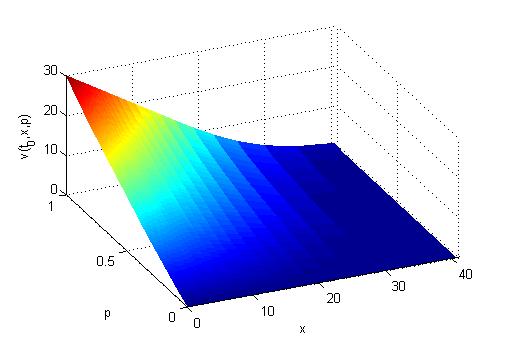
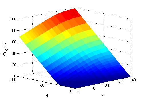
(a)	(b)

Figure 1: Surface of $v(t,x,p)$ and $v^{\sharp}(t,x,q)$ at $t=t_{0}$.

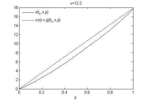
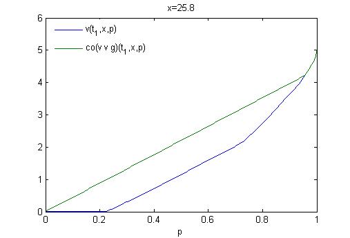
(a)	(b)
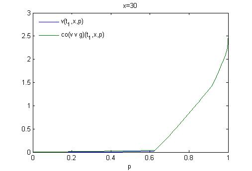
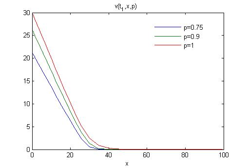
(c)	(d)

Figure 2: (a)-(c): plots of $v(t,x,\cdot)$ and ${\rm co}[v\vee g](t,x,\cdot)$ at $t=t_{1}$ and for different values of $x$. (d): plot of $v(t,\cdot,p)$ at $t=t_{1}$ and for different values of $p$.

In our second example, we consider a put spread option with strikes $20$ and $30$, i.e. $g(t,x)=[30-x]^{+}-[20-x]^{+}$. The numerical results are displayed in Figure 3 and 4. It may happen here that $v(t,x,1)<g(t,x)$, see figure 4(a).

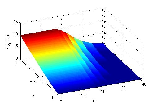
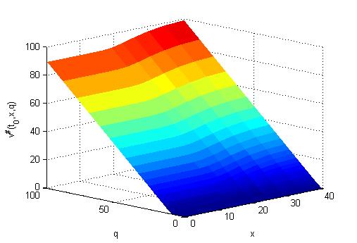
(a)	(b)

Figure 3: Surface of $v(t,x,p)$ and $v^{\sharp}(t,x,q)$ at $t=t_{0}$.

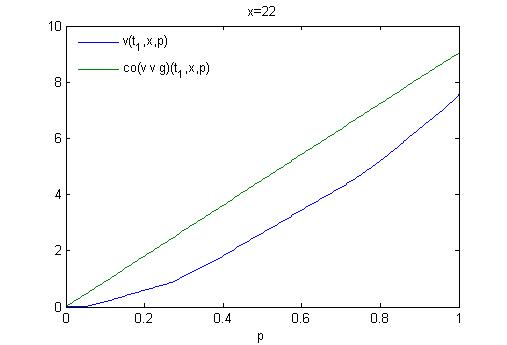
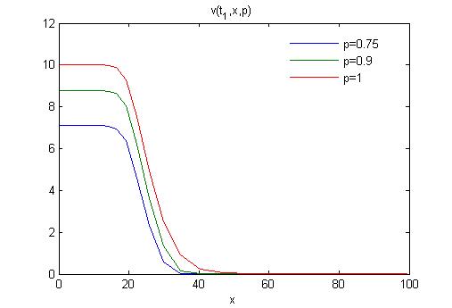
(a)	(b)

Figure 4: (a): plot of $v(t,x,\cdot)$ and ${\rm co}[v\!\vee\!g](t,x,\cdot)$ at $t=t_{1}$ and for $x=22$. (b): plot of $v(t,.,p)$ at $t=t_{1}$ and for different values of $p$.

We conclude this section with the following remark on the behavior of $v$ near ${p=}1$.

Remark 2.3.

(a) We know from the identification $v=w^{\sharp}$ and Proposition 3.2(b) that $p\mapsto v(t,x,p)$ is convex and continuous on $[0,1]$.
(b) Nothing prevents $\mathrm{D}^{-}_{p}v(\cdot,1)$ to be equal to $+\infty$. This can be checked by direct calculation in the European case and the Black-Scholes setting using the explicit formula [12, Equation (3.15)].

3 Proof of the backward dual representation

From now on, we extend $v$ to $[0,T]\times{\mathcal{O}}_{\!+}^{d}\times\mathbb{R}$ by setting

$$v(\cdot,p)=0\text{ if }p<0\text{ and }v(\cdot,p)=+\infty\text{ if }p>1\,.$$ (3.1)

Using the convention $\inf\emptyset=+\infty$, this extension is consistent with (2.7).

3.1 The backward algorithm as a lower bound

We first show that the backward algorithm (2.27) actually provides a lower bound for the value function $v$.

Proposition 3.1.

$v\geq w^{\sharp}$ on $[0,T]\times{\mathcal{O}}_{\!+}^{d}\times[0,1]$.

Proof. First note that $v(T,\cdot)=0=w^{\sharp}(T,\cdot)$, by definition. Thus, $(v\vee g)(T,\cdot)=(w^{\sharp}\vee g)(T,\cdot)$. We now assume that $v\geq w^{\sharp}$ on $[t_{i+1},T]\times{\mathcal{O}}_{\!+}^{d}\times[0,1]$ for some $i\leq n-1$. Then, $(v\!\vee\!g)^{\sharp}(t_{i+1},\cdot)\leq(w^{\sharp}\!\vee\!g)^{\sharp}(t_{i+1},\cdot)$ and therefore

$$(v\!\vee\!g)\left(t_{i+1},X^{t,x}_{t_{i+1}},P^{t,p,\alpha}_{t_{i+1}}\right) \geq P^{t,p,\alpha}_{t_{i+1}}qQ^{t,x,{1}}_{t_{i+1}}-(v\!\vee\!g)^{\sharp}\left(t_{i+1},X^{t,x}_{t_{i+1}},qQ^{t,x,{1}}_{t_{i+1}}\right)$$

$$\geq P^{t,p,\alpha}_{t_{i+1}}qQ^{t,x,{1}}_{t_{i+1}}-(w^{\sharp}\!\vee\!g)^{\sharp}\left(t_{i+1},X^{t,x}_{t_{i+1}},qQ^{t,x,{1}}_{t_{i+1}}\right)\,.$$

Fix $t\in[t_{i},t_{i+1})$. Taking the expectation on both sides and recalling (2.27), we obtain

$$\mathbb{E}^{\mathbb{Q}_{{t,x}}}\left[(v\!\vee\!g)\left(t_{i+1},X^{t,x}_{t_{i+1}},P^{t,p,\alpha}_{t_{i+1}}\right)\right]\geq pq-w(t,x,q)\,.$$

Taking first the supremum over $q\in\mathbb{R}$ in the right-hand side and then the infimum over $\alpha\in\mathcal{A}_{t,p}$ in the left-hand side, we get from Proposition 2.3 that $v(t,x,p)\geq w^{\sharp}(t,x,p)$. $\Box$

3.2 Representation and differentiability of the backward dual algorithm

This section is devoted to the study of the function $(w^{\sharp}\!\vee\!g)^{\sharp}$ which appears in the dual algorithm (2.27) and of its Fenchel transform $(w^{\sharp}\!\vee\!g)^{\sharp\sharp}$. We first provide a decomposition in simple terms in Proposition 3.3. They only contain $w,g$ and auxiliary functions that are easy to handle, see (3.3)-(3.4) below. In view of (2.27), this will then allow us to study the subdifferential of $w(t_{i},\cdot)$ in terms of the subdifferential of $w(t_{i+1},\cdot)$. This analysis is reported in Lemma 3.2. These results will be of important use in the final proof of Theorem 2.1 as it will require to find a particular value $p$ in the subdifferential of $w(t_{i},\cdot)$ and then to apply a martingale representation argument between elements of the subdifferential of $(w^{\sharp}\!\vee\!g)^{\sharp}$ at $t_{i+1}$ and $p$ at $t_{i}$, see the proof of Theorem 3.1.

We start with properties that stem directly from the definition of $w$ and standard results in convex analysis. The proof is postponed to the Appendix.

Proposition 3.2.

The following holds for all $(t,x)\in[0,T]\times{\mathcal{O}}_{\!+}^{d}$.

(a) The functions $q\in\mathbb{R}\mapsto w(t,x,q)$ is a proper convex non-decreasing and non-negative function. Moreover, $w(\cdot,0)=0$ and $w(\cdot,q)=\infty$ for $q<0$.

(b) The function $p\in\mathbb{R}\mapsto w^{\sharp}(t,x,p)$ and $q\in\mathbb{R}\mapsto(w^{\sharp}\!\vee\!g)^{\sharp}(t,x,q)$ are convex, non-negative, non-decreasing and continuous on their respective domains. Moreover, $w^{\sharp}(\cdot,0)=0=(w^{\sharp}\!\vee\!g)^{\sharp}(\cdot,0)$ and $(w^{\sharp}\!\vee\!g)^{\sharp}(\cdot,q)=+\infty$ for $q<0$.

The next result is key to get the representation of $(w^{\sharp}\vee g)^{\sharp}$ and $(w^{\sharp}\vee g)^{\sharp\sharp}$. Recall that $g(t,x,p)=g(t,x)\mathbf{1}_{\{0<p\leq 1\}}+\infty\mathbf{1}_{\{p>1\}}$.

Lemma 3.1.

Let $p_{1}\geq 0$ and $f$ be a non-decreasing convex function such that $f(0)=0$, $f\geq g(t,x,\cdot)$ on $[p_{1},\infty)$, $f\leq g(t,x,\cdot)$ on $(-\infty,p_{1}]$.
(a) The convex envelope of $f\vee g$ is given by

$${(f\!\vee\!g)^{\sharp\sharp}(p)=}{\rm co}[f\!\vee\!g](p)=pq_{1}\mathbf{1}_{\{0\leq p<p_{1}\}}+f(p)\mathbf{1}_{\{p_{1}\leq p\leq 1\}}+\infty\mathbf{1}_{\{{p>1}\}}\,,$$

with $q_{1}=g(t,x)/p_{1}\mathbf{1}_{\left\{p_{1}>0\right\}}$.
(b) Moreover, we have

$$(f\!\vee\!g)^{\sharp}(\cdot,q)=p_{1}[q-q_{1}]^{+}\mathbf{1}_{\left\{q{\leq}\mathrm{D}^{+}_{p}f(p_{1})\right\}}+f^{\sharp}(q)\mathbf{1}_{\left\{q{>}\mathrm{D}^{+}_{p}f(p_{1})\right\}}\,,\;q\geq 0\,,$$

which is a closed proper convex function. In particular, it is continuous at $\mathrm{D}^{+}_{p}f(p_{1})$ when $0<\mathrm{D}^{+}_{p}f(p_{1})<+\infty$.

Proof.
1. The left-hand side identity in (a) follows from [15, Theorem 12.2]. We set $\varphi:p\mapsto pq_{1}\mathbf{1}_{\{p>0\}}\vee f(p)$, which is convex. By assumption, we already know that $f(p)\leq g(t,x,p)=0$ for $p\leq 0$. Since $f(0)=0$ and $f(p_{1})=g(t,x)$, we have by convexity that $f(p)\leq pq_{1}$, $p\in[0,p_{1}]$, which implies $\varphi(p)\mathbf{1}_{\left\{p\leq p_{1}\right\}}=pq_{1}\mathbf{1}_{\{0\leq p\leq p_{1}\}}$, for $p\leq p_{1}$. Since $f(p)\leq pq_{1}$ for $p\in[0,p_{1}]$ and $f(p_{1})=p_{1}q_{1}$, we compute that $\mathrm{D}^{-}_{p}f(p_{1})\geq q_{1}$. By convexity, we also have $f(p)\geq f(p_{1})+\mathrm{D}^{-}_{p}f(p_{1})(p-p_{1})\geq pq_{1}$ for $p\geq p_{1}$ and then $\varphi\mathbf{1}_{[p_{1},\infty)}=f\mathbf{1}_{[p_{1},\infty)}$. In particular, we observe that $\varphi\leq f\!\vee\!g$. It is straightforward to check that any candidate for the convex envelope of $f\!\vee\!g$ is below $\varphi$. The above shows also that $\mathrm{D}^{+}_{p}f(p_{1})>0$ whenever $q_{1}>0$.
2. Let us now observe that $f^{\sharp}(q)<\infty$, for $q\geq 0$, since $f(\cdot,p)=g(\cdot,p)=\infty$ for $p>1\vee p_{1}$. It follows that the subdifferential of $f^{\sharp}$ at non-negative $q$ is non empty. The proof of (b) follows from calculations based on the following results from convex analysis, see e.g. [11, Chapter I Proposition 5.1]. Let $\psi$ be a proper function on $\mathbb{R}$, then $p$ is in the subdifferential of $\psi$ at $q$ if and only if

$$\psi^{\sharp}(p)+\psi(q)=pq\,.$$ (3.2)

(i) At $p=0$, the subdifferential of $(f\!\vee\!g)^{\sharp\sharp}={\rm co}[f\!\vee\!g]$ is equal to $[0,q_{1}]$. This follows directly from the characterization of the convex envelope of $f\!\vee\!g$ given in (a). Using the above equality with $\psi=(f\!\vee\!g)^{\sharp}$, we then have for $q\in[0,q_{1}]$

$$(f\!\vee\!g)^{\sharp\sharp}(0)+(f\!\vee\!g)^{\sharp}(q)=0\times q\implies(f\!\vee\!g)^{\sharp}(q)=0\,,$$

since $(f\!\vee\!g)^{\sharp\sharp}(0)=0$ by our assumption, namely $f(0)=0=g(\cdot,0)$ and $g\geq 0$.
(ii) The subdifferential of $(f\!\vee\!g)^{\sharp\sharp}={\rm co}[f\!\vee\!g]$ at $p_{1}$ is equal to $\mathcal{D}:=[q_{1},\mathrm{D}^{+}_{p}f(p_{1})]$ if $\mathrm{D}^{+}_{p}f(p_{1})<+\infty$ or $[q_{1},+\infty)$ otherwise. This follows again directly from (a). We recall from the step 1. that $f(p_{1})=q_{1}p_{1}$. Then, using (3.2) with $\psi=(f\!\vee\!g)^{\sharp}$ and (a), we have for $q\in\mathcal{D}$

$$(f\!\vee\!g)^{\sharp\sharp}(p_{1})+(f\!\vee\!g)^{\sharp}(q)=p_{1}q\implies(f\!\vee\!g)^{\sharp}(q){=p_{1}q-f(p_{1})}=p_{1}(q-q_{1}){=p_{1}[q-q_{1}]^{+}}\,.$$

(iii) If $q>\mathrm{D}^{+}_{p}f(p_{1})$, an element $p$ of the subdifferential of $f^{\sharp}$ at $q$ satisfies

$$f(p)+f^{\sharp}(q)=pq\,.$$

We first note that $p\geq p_{1}$ necessarily. Indeed, by [11, Chapter I Corollary 5.2], $q\in[\mathrm{D}^{-}_{p}f(p),\mathrm{D}^{+}_{p}f(p)]$ while $q>\mathrm{D}^{+}_{p}f(p_{1})$. Recall that $f=(f\!\vee\!g)^{\sharp\sharp}$ on $[p_{1},\infty)$. We then deduce from the previous equality that

$$(f\!\vee\!g)^{\sharp\sharp}(p)+f^{\sharp}(q)=pq\implies f^{\sharp}(q){=pq-(f\!\vee\!g)^{\sharp\sharp}(p)}\leq(f\!\vee\!g)^{\sharp}(q)\,.$$

Observing that the reverse inequality follows from $f\leq f\!\vee\!g$, we get $f^{\sharp}(q)=(f\!\vee\!g)^{\sharp}(q)$ for $q\in{(\mathrm{D}^{+}_{p}f(p_{1})},+\infty)$. $\Box$

We are now in position to provide the decomposition of $(w^{\sharp}\vee g)^{\sharp}$ and $(w^{\sharp}\vee g)^{\sharp\sharp}$. It basically follows from the application of the previous Lemma to $f=w^{\sharp}$.

Proposition 3.3.

For $(t,x,p)\in[0,T]\times{\mathcal{O}}_{\!+}^{d}\times\mathbb{R}$, we define the following ‘facelift’ of $g$

$$\tilde{g}(t,x,p)=q_{g}(t,x)p\mathbf{1}_{\{0\leq p\leq 1\}}+\infty\mathbf{1}_{\{p>1\}}\,.$$

with

$$q_{g}(t,x):=\frac{g(t,x)}{p_{g}(t,x)}\mathbf{1}_{\left\{p_{g}(t,x)>0\right\}}\;\mbox{ and }\;p_{g}(t,x):=\sup\left\{p\in\mathbb{R}\,|\,w^{\sharp}(t,x,p)=g(t,x)\right\}\;\wedge 1\,.$$

Then,

1. The function $q\mapsto(w^{\sharp}\!\vee\!g)^{\sharp\sharp}(\cdot,q)$ is continuous on its domain and

   $$(w^{\sharp}\!\vee\!g)^{\sharp\sharp} ={\rm co}[w^{\sharp}\!\vee\!g]=w^{\sharp}\!\vee\!\tilde{g}\,.$$ (3.3)

2. For all $q\in\mathbb{R}_{+}$:

   $$(w^{\sharp}\!\vee\!g)^{\sharp}(\cdot,q) =\left[q-g(\cdot)\right]^{+}\mathbf{1}_{A_{1}}(\cdot)+w(\cdot,q)\mathbf{1}_{A_{2}}(\cdot)+\kappa(\cdot,q)\mathbf{1}_{A_{3}}(\cdot)\,,$$ (3.4)

   where

   $$\kappa(\cdot,q) :=p_{g}(\cdot)\left[q-q_{g}(\cdot)\right]^{+}\mathbf{1}_{\left\{q\leq\bar{q}(\cdot)\right\}}+w(\cdot,q)\mathbf{1}_{\left\{q>\bar{q}(\cdot)\right\}}\,,$$

   with $\;\bar{q}(\cdot):=\mathrm{D}^{+}_{p}w^{\sharp}\left(\cdot,p_{g}(\cdot)\right)$ and the subsets of $\,[0,T]\times{\mathcal{O}}_{\!+}^{d}$: $A_{1}=\left\{g>0,\;{w^{\sharp}(\cdot,1)\leq g}\right\}$, $A_{2}=\left\{g=0\right\}$, $A_{3}=\left\{g>0,\;{w^{\sharp}(\cdot,1)>g}\right\}$.

Remark 3.1.

(a) It follows from Proposition 3.2 that $w^{\sharp}(\cdot,0)=0$. Hence, $g(t,x)>0$ implies $p_{g}(t,x)>0$ and

$$q_{g}(t,x) =\frac{g(t,x)}{p_{g}(t,x)}\mathbf{1}_{\left\{g(t,x)>0\right\}}\text{ so that }q_{g}(t,x)=0\mbox{ if and only if }g(t,x)=0\,.$$

(b) The decomposition on $A_{1}$, $A_{2}$ and $A_{3}$ will be useful in the sequel, see e.g. proof of Lemma 3.2(c) below.
(c) On $A_{3}$, we have $\bar{q}>0$ since $w^{\sharp}(\cdot,p_{g}(\cdot))\geq g>0$ and $w^{\sharp}(\cdot,0)=0$, see Proposition 3.2.

Proof of Proposition 3.3. The identities in (3.3) are immediate consequences of Lemma 3.1(a), Proposition 3.2(b) and of the definition of $p_{g}$. We now prove (3.4). For $(t,x)\in A_{1}$, we have $w^{\sharp}(t,x,\cdot)\leq g$ and therefore $(w^{\sharp}\!\vee\!g)^{\sharp}(t,x,\cdot)=g^{\sharp}(t,x,\cdot)$ $=$ $[\cdot-g(t,x)]^{+}$ on $\mathbb{R}_{+}$. For $(t,x)\in A_{2}$, we have that $w^{\sharp}\geq g$ by Proposition 3.2(b) and the result follows directly. On $A_{3}$, the expression is exactly the one given by Lemma 3.1(b). $\Box$

We can now turn to the study of the subdifferential of $w$. Recall the definition of $p_{\rm min}$ in (2.13).

Lemma 3.2.

Fix $0\leq i\leq n-1$ and $(t,x)\in[t_{i},t_{i+1})\times{\mathcal{O}}_{\!+}^{d}$. Then:
(a) $\mathrm{D}^{+}_{q}w(t,x,\cdot)\geq 0$ if $q\geq 0$ and $\mathrm{D}^{-}_{q}w(t,x,\cdot)\geq 0$ if $q>0$,
(b) $\lim_{q\uparrow\infty}\mathrm{D}^{+}_{q}w(t,x,q)=1$,
(c) $\mathrm{D}^{+}_{q}w(t,x,0)=p_{\rm min}(t,x)$.
Moreover,

$$\mathrm{D}^{-}_{q}w(t,x,q) =\mathbb{E}\left[\mathrm{D}^{-}_{q}(w^{\sharp}\!\vee\!g)^{\sharp}(t_{i+1},X^{t,x}_{t_{i+1}},qQ^{t,x,1}_{t_{i+1}}))\right]\,\;\text{ for }q>0\,,\;\text{ and }$$ (3.5)

$$\mathrm{D}^{+}_{q}w(t,x,q) =\mathbb{E}\left[\mathrm{D}^{+}_{q}(w^{\sharp}\!\vee\!g)^{\sharp}(t_{i+1},X^{t,x}_{t_{i+1}},qQ^{t,x,1}_{t_{i+1}}))\right]\,\;\text{ for }q\geq 0\,.$$ (3.6)

Proof. The proof is based on an induction argument. Our assumptions guarantee that (a)-(b)-(c) are valid at $T$. Let us assume that it holds true on $[t_{i+1},T]$ for some $i\leq n-1$.

In view of Proposition 3.3, we obtain for $q\geq 0$ and $j\leq n$ that

$$\mathrm{D}^{+}_{q}(w^{\sharp}\!\vee\!g)^{\sharp}(t_{j},x,q) =\mathbf{1}_{\left\{q\geq g(t_{j},x)\right\}}\mathbf{1}_{A_{1}}(t_{j},x)+\mathrm{D}^{+}_{q}w(t_{j},x,q)\mathbf{1}_{A_{2}}(t_{j},x)$$

$$\quad+\mathrm{D}^{+}_{q}\kappa(t_{j},x,q)\mathbf{1}_{A_{3}}(t_{j},x)\,,$$

with

$$\mathrm{D}^{+}_{q}\kappa(t_{j},x,q)=p_{g}(t_{j},x)\mathbf{1}_{\left\{q_{g}(t_{j},x)\leq q<\bar{q}(t_{j},x)\right\}}+\mathrm{D}^{+}_{q}w(t_{j},x,q)\mathbf{1}_{\left\{q>\bar{q}(t_{j},x)\right\}}\,.$$

For $q>0$, we have

$$\mathrm{D}^{-}_{q}(w^{\sharp}\!\vee\!g)^{\sharp}(t_{j},x,q) =\mathbf{1}_{\left\{q>g(t_{j},x)\right\}}\mathbf{1}_{A_{1}}(t_{j},x)+\mathrm{D}^{-}_{q}w(t_{j},x,q)\mathbf{1}_{A_{2}}(t_{j},x)$$

$$\quad+\mathrm{D}^{-}_{q}\kappa(t_{j},x,q)\mathbf{1}_{A_{3}}(t_{j},x)\,,$$

with

$$\mathrm{D}^{-}_{q}\kappa(t_{j},x,q)=p_{g}(t_{j},x)\mathbf{1}_{\left\{q_{g}(t_{j},x)<q\leq\bar{q}(t_{j},x)\right\}}+\mathrm{D}^{-}_{q}w(t_{j},x,q)\mathbf{1}_{\left\{q>\bar{q}(t_{j},x)\right\}}\,.$$

We have by induction $\lim_{q\uparrow\infty}\mathrm{D}^{+}_{q}\kappa(t_{i+1},x,q)=1$, which ensures that $\lim_{q\uparrow\infty}\mathrm{D}^{+}_{q}(w^{\sharp}\!\vee\!g)^{\sharp}(t_{i+1},x,q)=1$. By the convexity of $(w^{\sharp}\!\vee\!g)^{\sharp}$, this implies that $\mathrm{D}^{+}_{q}(w^{\sharp}\!\vee\!g)^{\sharp}(t_{i+1},x,q)\leq 1$. In view of (2.27), a dominated convergence argument then leads to (3.5)-(3.6) and $\lim_{q\uparrow+\infty}\mathrm{D}^{+}_{q}w(t,x,q)=1$.

We now use our induction hypothesis again to observe from the decomposition above that

$$\mathrm{D}^{-}_{q}(w^{\sharp}\!\vee\!g)^{\sharp}(t_{i+1},x,q)\geq 0\,,\;q>0\,,\;\text{ and }\;\mathrm{D}^{+}_{q}(w^{\sharp}\!\vee\!g)^{\sharp}(t_{i+1},x,q)\geq 0\,,\;q\geq 0\,.$$

Recalling (3.5)-(3.6), this shows that $\mathrm{D}^{-}_{q}w(t,x,q)\geq 0$ for $q>0$ and $\mathrm{D}^{+}_{q}w(t,x,q)\geq 0$ for $q\geq 0$.

It remains to prove (c). From Remark 3.1(a) and (c), the above decomposition implies that $\mathrm{D}^{+}_{q}(w^{\sharp}\!\vee\!g)^{\sharp}(t_{i+1},x,0)$ $=$ $\mathrm{D}^{+}_{q}w(t_{i+1},x,0)\mathbf{1}_{\{g(t_{i+1},x)=0\}}$. By our induction hypothesis, the last term is $\mathrm{D}^{+}_{q}(w^{\sharp}\!\vee\!g)^{\sharp}(t_{i+1},x,0)$ $=$ $p_{\rm min}(t_{i+1},x)\mathbf{1}_{\{g(t_{i+1},x)=0\}}$. This identity combined with (3.6) provides

$$\mathrm{D}^{+}_{q}w(t,x,0) =\mathbb{E}\!\!\left[p_{\rm min}(t_{i+1},X^{t,x}_{t_{i+1}})\mathbf{1}_{\left\{g(t_{i+1},X^{t,x}_{t_{i+1}})=0\right\}}\right]=p_{\rm min}(t,x)\,,$$

in which the last identity is an obvious consequence of the definition of $p_{\rm min}$ in (2.13). $\Box$

Remark 3.2.

Note that the subdifferential of $w(t,x,\cdot)$ at $0$ is $(-\infty,p_{{\rm min}}(t,x)]$, since $w(t,x,q)=\infty$ for $q<0$ and $\mathrm{D}^{+}_{q}w(t,x,0)=p_{{\rm min}}(t,x)$. See (a) of Proposition 3.2 and (c) of Lemma 3.2.

3.3 The backward algorithm as an upper-bound

Our final proof will proceed by backward induction on the time steps. Fix $0\leq i\leq n-1$. Part of the induction hypothesis is:

Hypothesis (${\rm H_{i+1}}$).

The following holds

1. The functions $v(t_{i+1},\cdot)$ and ${\rm co}[v\!\vee\!g](t_{i+1},\cdot)$ are continuous on ${\mathcal{O}}_{\!+}^{d}\times[0,1]$.

2. ${\rm co}[v\!\vee\!g](t_{i+1},\cdot,0)=0$ and ${\rm co}[v\!\vee\!g](t_{i+1},\cdot,1)=(v\!\vee\!g)(t_{i+1},\cdot,1)$.

3. For all $x\in{\mathcal{O}}_{\!+}^{d}$, the map $q\in\mathbb{R}_{+}\mapsto q-(w^{\sharp}\!\vee\!g)^{\sharp}(t_{i+1},x,q)$ is non-decreasing, continuous and converges to $(v\!\vee\!g)(t_{i+1},x,1)$ as $q\to\infty$.

Before turning to the final argument, we provide three additional results that hold at any time $t\in[t_{i}{},t_{i+1})$ whenever ${\rm H_{i+1}}$ is in force.

3.3.1 Bounds and limits for $w^{\sharp}$

Our first additional result concerns the behavior of $w^{\sharp}$. It shows that $w^{\sharp}(t_{i},x,1)=v(t_{i},x,1)$. The last assertion will be used in the proof of Lemma 3.4 below to show that (iii) of ${\rm H_{i}}$ holds if (iii) of ${\rm H_{i+1}}$ does.

Lemma 3.3.

Let iii of ${\rm H_{i+1}}$ hold. Fix $(t,x)\in[t_{i}{},t_{i+1})\times{\mathcal{O}}_{\!+}^{d}$. Then, $w^{\sharp}(t,x,\cdot)$ is non-negative, continuous on its domain $(-\infty,1]$ and

$$0\leq w^{\sharp}(t,x,\cdot)\leq w^{\sharp}(t,x,1)=v(t,x,1)\;\mbox{ on }(-\infty,1]\,.$$

Moreover, the map $q\in\mathbb{R}\mapsto q-w(t,x,q)$ is non-decreasing, continuous on $\mathbb{R}_{+}$ and converges to $v(t,x,1)$ as $q\to\infty$.

Proof. The continuity and non-negativity of $w^{\sharp}(t,x,\cdot)$ are stated in (b) of Proposition 3.2. We now observe that (2.27) implies that

$$\delta(q):=q-w(t,x,q)=\mathbb{E}^{\mathbb{Q}_{t,x}}\left[qQ^{t,x,1}_{t_{i+1}}-(w^{\sharp}\!\vee\!g)^{\sharp}(t_{i+1},X^{t,x}_{t_{i+1}},qQ^{t,x,1}_{t_{i+1}})\right]\,,$$

which shows that $q\mapsto\delta(q)$ is non-decreasing since (iii) of ${\rm H_{i+1}}$ holds. Applying the monotone convergence Theorem, iii of ${\rm H_{i+1}}$ and (2.9), we obtain that $q\in\mathbb{R}_{+}\mapsto q-w(t,x,q)$ is continuous and that

$$\lim_{q\rightarrow\infty}\delta(q)=\mathbb{E}^{\mathbb{Q}_{t,x}}\left[(v\!\vee\!g)(t_{i+1},X^{t,x}_{t_{i+1}},1)\right]=v(t,x,1)\,.$$

This implies that $w^{\sharp}(t_{i},x,1)=\sup_{q\geq 0}\delta(q)$ $\geq$ $\lim_{q\to\infty}\delta(q)$ $=$ $v(t,x,1)$, while $w^{\sharp}(t,x,p)\geq\lim_{q\to\infty}(q(p-1)+\delta(q))$ $=$ $\infty$ for $p>1$. The fact that $w^{\sharp}(t_{i},x,1)\leq v(t,x,1)$ has been proved in Proposition 3.1. $\Box$

3.3.2 Convexification in the dynamic programming algorithms

As already mentioned in Remark 2.2, one can expect that $v\vee g$ can be replaced by its convex envelope, with respect to $p$, in (2.18). The Hypotheses i-ii of ${\rm H_{i+1}}$ ensure this, see Proposition 3.4 below. We shall prove a similar result for $w^{\sharp}$ later on in Theorem 3.1. Note that the two identities (3.7) and (3.11) below already suggest that the equality $v=w^{\sharp}$ at $t_{i+1}$ should iterate at $t_{i}$, since we already know from Proposition 3.1 that $v\geq w^{\sharp}$.

Proposition 3.4.

Let (i)-(ii) of ${\rm H_{i+1}}$ hold. Then, for all $t\in[t_{i},t_{i+1})$ and $(x,p)\in{\mathcal{O}}_{\!+}^{d}\times[0,1]$, we have

$$v(t,x,p)=\inf_{\alpha\in\mathcal{A}_{t,p}}\mathbb{E}^{\mathbb{Q}_{t,x}}\left[{\rm co}[v\!\vee\!g]\left(t_{i+1},X^{t,x}_{t_{i+1}},P^{t,p,\alpha}_{t_{i+1}}\right)\right]\,.$$ (3.7)

Moreover, ii of ${\rm H_{i}}$ holds.

Proof. We fix $(t,x)\in[t_{i},t_{i+1})\times{\mathcal{O}}_{\!+}^{d}$. Assuming that (3.7) is true, we deduce that ii of ${\rm H_{i}}$ holds, since $\mathcal{A}_{t,p}=\{0\}$ for $p\in\{0,1\}$ and therefore $P^{t,p,\alpha}_{t_{i+1}}=p$ for $\alpha\in\mathcal{A}_{t,p}$. By ii of ${\rm H_{i+1}}$, the same argument combined with Proposition 2.3 implies that (3.7) is valid for $p\in\{0,1\}$.

It remains to prove (3.7) for $0<p<1$. In view of Proposition 2.3, this reduces to showing that

$$\inf_{\alpha\in\mathcal{A}_{t,p}}\mathbb{E}^{\mathbb{Q}_{t,x}}\left[{\rm co}[v\!\vee\!g]\left(t_{i+1},X^{t,x}_{t_{i+1}},P^{t,p,\alpha}_{t_{i+1}}\right)\right]\geq\inf_{\alpha\in\mathcal{A}_{t,p}}\mathbb{E}^{\mathbb{Q}_{t,x}}\left[({v\!\vee\!g})\left(t_{i+1},X^{t,x}_{t_{i+1}},P^{t,p,\alpha}_{t_{i+1}}\right)\right]\,,$$

the reverse inequality being trivial. We argue as in [5, Proof of Proposition 3.3]. It follows from the Caratheodory theorem that we can find two maps $(\lambda_{j},\pi_{j}):(x,p)\in{\mathcal{O}}_{\!+}^{d}\times[0,1]\mapsto(\lambda_{j},\pi_{j})(x,p)\in{\mathcal{O}}_{\!+}^{d}\times[0,1]$, $j\leq 2$, such that

$$\begin{array}[]{c}\sum_{j=1}^{2}\pi_{j}(x,p)=1\mbox{ , }p=\sum_{j=1}^{2}\pi_{j}(x,p)\lambda_{j}(x,p)\\ \mbox{ and }\;{\rm co}[v\!\vee\!g](t_{i+1},x,p)=\sum_{j=1}^{2}\pi_{j}(x,p)(v\!\vee\!g)(t_{i+1},x,\lambda_{j}(x,p))\,.\end{array}$$ (3.10)

We claim that they can be chosen in a measurable way. More precisely, i of ${\rm H_{i+1}}$ and [4, Proposition 7.49] imply that they can be chosen to be analytically measurable. We can then appeal to [4, Lemma 7.27] to obtain a Borel-measurable version which coincides a.e. for the pull-back measure of $(X^{t,x}_{t_{i+1}-\varepsilon},P^{t,p,\alpha}_{t_{i+1}-\varepsilon})$, for $\alpha\in\mathcal{A}_{t,p}$ and $0<\varepsilon<t_{i+1}-t$ fixed. This is this version that we use in the following.

We now let $\xi$ be a $\mathcal{F}_{t_{i+1}}$-measurable random variable such that

$$\mathbb{P}[\xi=\lambda_{j}(X^{t,x}_{t_{i+1}-\varepsilon},P^{t,p,\alpha}_{t_{i+1}-\varepsilon})|\mathcal{F}_{t_{i+1}-\varepsilon}]=\pi_{j}(X^{t,x}_{t_{i+1}-\varepsilon},P^{t,p,\alpha}_{t_{i+1}-\varepsilon})\,.$$

Then, $\mathbb{E}[\xi|\mathcal{F}_{t_{i+1}-\varepsilon}]=P^{t,p,\alpha}_{t_{i+1}-\varepsilon}$ by the above construction, and we can then find $\alpha_{\varepsilon}\in\mathcal{A}_{t,p}$ such that $P^{t,p,\alpha_{\varepsilon}}_{t_{i+1}-\varepsilon}=P^{t,p,\alpha}_{t_{i+1}-\varepsilon}$ and $P^{t,p,\alpha_{\varepsilon}}_{t_{i+1}}=\xi$. Recalling (3.10), we obtain

$$\mathbb{E}\left[\left(Q^{t,x,1}_{t_{i+1}-\varepsilon}\right)^{-1}{\rm co}[v\!\vee\!g]\left(t_{i+1},X^{t,x}_{t_{i+1}-\varepsilon},P^{t,p,\alpha}_{t_{i+1}-\varepsilon}\right)\right]$$

$$=\mathbb{E}^{\mathbb{Q}_{t,x}}\left[({v\!\vee\!g})\left(t_{i+1},X^{t,x}_{t_{i+1}-\varepsilon},P^{t,p,\alpha_{\varepsilon}}_{t_{i+1}}\right)\right]$$

$$\quad-\mathbb{E}\left[\left(\left(Q^{t,x,1}_{t_{i+1}}\right)^{-1}-\left(Q^{t,x,1}_{t_{i+1}-\varepsilon}\right)^{-1}\right)({v\!\vee\!g})\left(t_{i+1},X^{t,x}_{t_{i+1}-\varepsilon},P^{t,p,\alpha_{\varepsilon}}_{t_{i+1}}\right)\right]$$

$$\geq\inf_{\alpha^{\prime}\in\mathcal{A}_{t,p}}\mathbb{E}^{\mathbb{Q}_{t,x}}\left[({v\!\vee\!g})\left(t_{i+1},X^{t,x}_{t_{i+1}},P^{t,p,\alpha^{\prime}}_{t_{i+1}}\right)\right]+\Delta(\epsilon)\,,$$

with

$$\Delta(\epsilon) =-C\mathbb{E}^{\mathbb{Q}_{t,x}}\left[\left(1+|X^{t,x}_{t_{i+1}-\varepsilon}|+|X^{t,x}_{t_{i+1}}|\right)\left|X^{t,x}_{t_{i+1}-\varepsilon}-X^{t,x}_{t_{i+1}}\right|\right]$$

$$\quad-C\mathbb{E}\left[\left(\left(Q^{t,x,1}_{t_{i+1}}\right)^{-1}-\left(Q^{t,x,1}_{t_{i+1}-\varepsilon}\right)^{-1}\right)\left(1+|X^{t,x}_{t_{i+1}-\varepsilon}|\right)\right]\,,$$

recall (2.6), (2.16) and (2.19). Moreover, since $0\leq{\rm co}[v\!\vee\!g](t_{i+1},x,\cdot)\leq{v\!\vee\!g}(t_{i+1},x,\cdot)\leq C(1+|x|)$, using i of ${\rm H_{i+1}}$, we can pass to the limit to obtain

$$\mathbb{E}^{\mathbb{Q}_{t,x}}\left[{\rm co}[v\!\vee\!g]\left(t_{i+1},X^{t,x}_{t_{i+1}},P^{t,p,\alpha}_{t_{i+1}}\right)\right] \geq \inf_{\alpha^{\prime}\in\mathcal{A}_{t,p}}\mathbb{E}^{\mathbb{Q}_{t,x}}\left[({v\!\vee\!g})\left(t_{i+1},X^{t,x}_{t_{i+1}},P^{t,p,\alpha^{\prime}}_{t_{i+1}}\right)\right]\,.$$

$\Box$

Since our final result is $v=w^{\sharp}$, the same convexification should appear in the dual algorithm. As already mentioned, it will actually allow us to show that $v=w^{\sharp}$ at $t_{i}$ if this true at $t_{i+1}$.

Theorem 3.1.

Let iii of ${\rm H_{i+1}}$ hold. Fix $(t,x,p)\in[t_{i}{},t_{i+1})\times{\mathcal{O}}_{\!+}^{d}\times[0,1]$. Then, there exists $\bar{\alpha}\in\mathcal{A}_{t,p}$ such that

$$w^{\sharp}(t,x,p) =\mathbb{E}^{\mathbb{Q}_{t,x}}\left[{\rm co}[w^{\sharp}\!\vee\!g]\left(t_{i+1},X^{t,x}_{t_{i+1}},P^{t,p,\bar{\alpha}}_{t_{i+1}}\right)\right]\,.$$ (3.11)

Proof. Recall the definition of $p_{\rm min}$ in (2.13).

1. We first assume that $p\in(p_{\rm min}(t,x),1)$. We know from Lemma 3.2(b)-(c) that there exists a $\tilde{q}\in(0,\infty)$ such that $p$ lies in the subdifferential of $w(t,x,\cdot)$ at $\tilde{q}$. Then, we can find $\lambda\in[0,1]$ such that $p=\lambda\mathrm{D}^{+}_{q}w(t,x,\tilde{q})+(1-\lambda)\mathrm{D}^{-}_{q}w(t,x,\tilde{q})$. In view of (3.5)-(3.6), this implies that

$$p =\mathbb{E}\left[(\lambda\mathrm{D}^{+}_{q}(w^{\sharp}\!\vee\!g)^{\sharp}+(1-\lambda)\mathrm{D}^{-}_{q}(w^{\sharp}\!\vee\!g)^{\sharp})\left(t_{i+1},X^{t,x}_{t_{i+1}},\tilde{q}Q^{t,x,{1}}_{t_{i+1}}\right)\right]\,.$$ (3.12)

It follows from Lemma 3.2 and its proof that the random variable in the expectation is valued in $[0,1]$. By the martingale representation theorem, we can find $\bar{\alpha}\in\mathcal{A}_{t,p}$ such that

$$(\lambda\mathrm{D}^{+}_{q}(w^{\sharp}\!\vee\!g)^{\sharp}+(1-\lambda)\mathrm{D}^{-}_{q}(w^{\sharp}\!\vee\!g)^{\sharp})\left(t_{i+1},X^{t,x}_{t_{i+1}},\tilde{q}Q^{t,x,{1}}_{t_{i+1}}\right)=p+\int_{t}^{t_{i+1}}\bar{\alpha}_{s}^{\top}\mathrm{d}W_{s}=:P^{t,p,\bar{\alpha}}_{t_{i+1}}\,.$$

For later use, note that the above implies

$$P^{t,p,\bar{\alpha}}_{t_{i+1}}\tilde{q}Q^{t,x,{1}}_{t_{i+1}}-(w^{\sharp}\!\vee\!g)^{\sharp}\left(t_{i+1},X^{t,x}_{t_{i+1}},\tilde{q}Q^{t,x,{1}}_{t_{i+1}}\right)=(w^{\sharp}\!\vee\!g)^{\sharp\sharp}\left(t_{i+1},X^{t,x}_{t_{i+1}},P^{t,p,\bar{\alpha}}_{t_{i+1}}\right)\,,$$ (3.13)

where we used (3.2) with $\psi=(w^{\sharp}\!\vee\!g)^{\sharp}$. On the other hand, we also have, again by (3.2) with $\psi=w$,

$$w(t,x,\tilde{q})+w^{\sharp}(t,x,p)=\tilde{q}p\,,$$ (3.14)

and, by (2.27),

$$w(t,x,\tilde{q})=\mathbb{E}^{\mathbb{Q}_{t,x}}\left[(w^{\sharp}\!\vee\!g)^{\sharp}\left(t_{i+1},X^{t,x}_{t_{i+1}},\tilde{q}Q^{t,x,{1}}_{t_{i+1}}\right)\right]\,.$$ (3.15)

Thus, inserting (3.12) and (3.15) into (3.14), and using (3.13), leads to

$$w^{\sharp}(t,x,p) =\mathbb{E}^{\mathbb{Q}_{t,x}}\left[P^{t,p,\bar{\alpha}}_{t_{i+1}}\tilde{q}Q^{t,x,{1}}_{t_{i+1}}-(w^{\sharp}\!\vee\!g)^{\sharp}\left(t_{i+1},X^{t,x}_{t_{i+1}},\tilde{q}Q^{t,x,{1}}_{t_{i+1}}\right)\right]$$

$$=\mathbb{E}^{\mathbb{Q}_{t,x}}\left[(w^{\sharp}\!\vee\!g)^{\sharp\sharp}\left(t_{i+1},X^{t,x}_{t_{i+1}},P^{t,p,\bar{\alpha}}_{t_{i+1}}\right)\right]\,.$$

We conclude by appealing to (3.3).

2. We now assume that $p\in[0,p_{{\rm min}}(t,x)]$. Since $[0,p_{{\rm min}}(t,x)]$ belongs to the subdifferential of $w(t,x,\cdot)$ at $0$, recall Remark 3.2, and $p_{{\rm min}}(t,x)=\mathrm{D}^{+}_{q}w(t,x,0)$, recall Lemma 3.2, we can find $\lambda\in[0,1]$ such that $p=\lambda\mathrm{D}^{+}_{q}w(t,x,0)$. We then proceed as above up to obvious modifications.

3. We finally assume that $p=1$. We know from Lemma 3.3 that $w^{\sharp}(t,x,1)=v(t,x,1)$. Hence, (2.9) implies

$$w^{\sharp}(t,x,1)=v(t,x,1) =\mathbb{E}^{\mathbb{Q}_{t,x}}\left[(v\!\vee\!g)\left(t_{i+1},X^{t,x}_{t_{i+1}},1\right)\right]\,.$$

As in the proof of Lemma 3.3, we deduce from iii of ${\rm H_{i+1}}$that ${\rm co}[w^{\sharp}\!\vee\!g](t_{i+1},\cdot,1)=(w^{\sharp}\!\vee\!g)^{\sharp\sharp}(t_{i+1},\cdot,1)\geq(v\!\vee\!g)(t_{i+1},\cdot,1)$. In view of Proposition 3.1, this leads to $(v\!\vee\!g)(t_{i+1},x,1)={\rm co}[w^{\sharp}\!\vee\!g](t_{i+1},x,1)$. $\Box$

3.4 Conclusion of the proof

To conclude the proof of Theorem 2.1, we need to prove the inequality $v\leq w^{\sharp}$.

Proposition 3.5.

$v\leq w^{\sharp}$ on $[0,T]\times{\mathcal{O}}_{\!+}^{d}\times[0,1]$.

Proof. We use a backward induction argument. We assume that ${\rm H_{i+1}}$ holds and that $v=w^{\sharp}$ and on $[t_{i+1},T]\times{\mathcal{O}}_{\!+}^{d}\times[0,1]$ for some $i\leq n-1$. Since it is true for $i=n$ by construction, the proof will be completed if one can show that this implies that ${\rm H_{i}}$ holds and that $v=w^{\sharp}$ on $[t_{i},T]\times{\mathcal{O}}_{\!+}^{d}\times[0,1]$.

Let us fix $(t,x,p)\in[t_{i},t_{i+1})\times{\mathcal{O}}_{\!+}^{d}\times[0,1]$. Then, our induction hypothesis implies that

$$\mathbb{E}^{\mathbb{Q}_{t,x}}\left[{\rm co}[v\!\vee\!g]\left(t_{i+1},X^{t,x}_{t_{i+1}},P^{t,p,\alpha}_{t_{i+1}}\right)\right]=\mathbb{E}^{\mathbb{Q}_{t,x}}\left[{\rm co}[w^{\sharp}\!\vee\!g]\left(t_{i+1},X^{t,x}_{t_{i+1}},P^{t,p,\alpha}_{t_{i+1}}\right)\right]\,,$$

for all $\alpha\in\mathcal{A}_{t,p}$. It then follows from Theorem 3.1 and Proposition 3.4 that $v(t,x,p)\leq w^{\sharp}(t,x,p)$. But, the reverse inequality is proved in Proposition 3.1. This shows that $v=w^{\sharp}$ on $[t_{i},T]\times{\mathcal{O}}_{\!+}^{d}\times[0,1]$. Then (i) of ${\rm H_{i}}$ is a consequence of Proposition 3.3 and Proposition 3.2. Proposition 3.4 implies (ii) of ${\rm H_{i}}$. Regarding the validity of (iii) of ${\rm H_{i}}$, it is proved in Lemma 3.4 below. $\Box$

Lemma 3.4.

The hypothesis ${\rm H_{i+1}}$ implies iii of ${\rm H_{i}}$.

Proof. It follows from (3.4) that

$$q-(w^{\sharp}\!\vee\!g)^{\sharp}(t_{i},x,q) =\big{(}q-[q-g(t_{i},x)]^{+}\big{)}{\mathbf{1}_{A_{1}}}(t_{i},x)$$

$$+(q-w(t_{i},x,q))\mathbf{1}_{A_{2}}(t_{i},x)+\big{(}q-\kappa(t_{i},x,q)\big{)}{\mathbf{1}_{A_{3}}}(t_{i},x)\,,$$ (3.16)

in which

$$q-\kappa(t_{i},x,q)=(q-p_{g}(t_{i},x)[q-q_{g}(t_{i},x)]^{+})\mathbf{1}_{\left\{q\leq\bar{q}(t_{i},x)\right\}}+(q-w(t_{i},x,q))\mathbf{1}_{\left\{q>\bar{q}(t_{i},x)\right\}}\,.$$

By Lemma 3.3, $w^{\sharp}(t_{i},x,1)=v(t_{i},x,1)$ so that $A_{2}\cup A_{3}=\left\{v(\cdot,1)>g\right\}$, recall (2.14). In particular, we observe that $\bar{q}<\infty$ on ${A_{3}}$. The fact that the right-hand side in (3.4) converges to $(v\!\vee\!g)(t_{i},x,1)$ as $q\to\infty$ is then a consequence of Lemma 3.3 and the definition of the $(A_{i})_{i\leq 3}$.

It remains to show that each term in (3.4) is non-decreasing and continuous. From Lemma 3.3, we know that $q\mapsto q-w(t_{i},x,q)$ is continuous and non-decreasing. The second term in the right-hand side of (3.4) is continuous and non-decreasing as well. As for the last term, we know that $q\mapsto\kappa(t_{i},x,q)$ is continuous, so that it suffices to check the monotony on each sub-interval $(-\infty,\bar{q}(t_{i},x)]$ and $[\bar{q}(t_{i},x),\infty)$ distinctly. On the second interval, we have that $q\mapsto q-\kappa(t_{i},x,q)$ is non-decreasing by Lemma 3.3. This is also true on first interval since $p_{g}(t_{i},x)\leq 1$. $\Box$

4 Appendix

We provide here the proofs of some technical results that were used in the proof of Theorem 2.1.

Proof of Proposition 2.1 For $t=T$ the sets in (2.12) are $\mathbb{R}_{+}$ by definition of $\mathbb{T}_{t}$ and ${\cal T}_{t}$. For $t<T$, the definition of $\hat{\tau}_{\nu}$ implies $\mathrm{S}^{t,x,y,\nu}_{\hat{\tau}_{\nu}}{=}\bigcap_{s\in\mathbb{T}_{t}}\mathrm{S}^{t,x,y,\nu}_{s}$, while $\bigcap_{s\in\mathbb{T}_{t}}\mathrm{S}^{t,x,y,\nu}_{s}\subset\mathrm{S}^{t,x,y,\nu}_{\tau}$, for any $\tau\in{\cal T}_{t}$. Hence, for $t<T$,

$${\mathbb{P}[\mathrm{S}^{t,x,y,\nu}_{\hat{\tau}_{\nu}}]\geq p\;\Rightarrow\;\mathbb{P}\left[\bigcap_{s\in\mathbb{T}_{t}}\mathrm{S}^{t,x,y,\nu}_{s}\right]\geq p\;\Rightarrow\;{\mathbb{P}[\mathrm{S}^{t,x,y,\nu}_{\tau}]\geq p,\;\forall\;\tau\in{\cal T}_{t}}\;\Rightarrow\;\mathbb{P}[\mathrm{S}^{t,x,y,\nu}_{\hat{\tau}_{\nu}}]\geq p,}$$

where, in the last implication, we used the fact that $\hat{\tau}_{\nu}\in{\cal T}_{t}$. This proves (2.12) for $t<T$. $\Box$

Proof of Proposition 2.3. 1. We first show that (2.18) holds. Let $\bar{v}(t,x,p)$ denote the right-hand side of (2.18) and set

$$J(t,x,p,\alpha):=\mathbb{E}^{\mathbb{Q}_{t,x}}\left[(v\!\vee\!g)\left(t_{i+1},X^{t,x}_{t_{i+1}},P^{t,p,\alpha}_{t_{i+1}}\right)\right]\,.$$

Fix $y$ and $\alpha\in\mathcal{A}_{t,p}$ such that $y>J(t,x,p,\alpha).$ Then, it follows from the martingale representation theorem that we can find $\nu\in\mathcal{U}_{t,x,y}$ such that

$$Y^{t,x,y,\nu}_{t_{i+1}}>(v\!\vee\!g)\left(t_{i+1},X^{t,x}_{t_{i+1}},P^{t,p,\alpha}_{t_{i+1}}\right)\,.$$

In particular, $Y^{t,x,y,\nu}_{t_{i+1}}\geq g\left(t_{i+1},X^{t,x}_{t_{i+1}},P^{t,p,\alpha}_{t_{i+1}}\right)$. Since, we also have $Y^{t,x,y,\nu}_{t_{i+1}}$ $>$ $v(t_{i+1},X^{t,x}_{t_{i+1}},$ $P^{t,p,\alpha}_{t_{i+1}})$, it follows from the same arguments as in the proof of [8, Lemma 2.2] that we can find a predictable process $(\tilde{\nu},\tilde{\alpha})$ which coincides with $(\nu,\alpha)$ on $[t,t_{i+1}]$, in the $\mathrm{d}t\times\mathrm{d}\mathbb{P}$-sense, and such that

$$Y^{t,x,y,\tilde{\nu}}_{s}\geq g\left(s,X^{t,x}_{s},P^{t,p,\tilde{\alpha}}_{s}\right)\,,\mbox{ for all }s\in\mathbb{T}_{t_{i+1}}\,.$$

These processes are elements of $\hat{\mathcal{U}}_{t,x,y,p}$ whenever $\tilde{\nu}$ is square integrable in the sense of (2.5) and $\tilde{\alpha}$ is such that $P^{t,p,\tilde{\alpha}}\in[0,1]$. The latter can be modified so that $P^{t,p,\tilde{\alpha}}$ is restricted to live in the interval $[0,1]$ while $\tilde{\nu}$ can be modified so that (2.15) holds. By the Itô isometry, this induces the required square integrability property of the financial strategy, recall (2.2)-(2.3). Combining the above with Proposition 2.2 shows that $\bar{v}(t,x,p)\geq v(t,x,p)$.

Conversely, let us fix $y>v(t,x,p)$. Then, it follows from the geometric dynamic programming principle of [8, Theorem 2.1] that there exists $(\nu,\alpha)\in\hat{\mathcal{U}}_{t,x,y,p}$ such that

$$Y^{t,x,y,\nu}_{t_{i+1}}\geq(v\vee g)\left(t_{i+1},X^{t,x}_{t_{i+1}},P^{t,p,\alpha}_{t_{i+1}}\right)\,.$$

Since $Y^{t,x,y,\nu}$ is a super-martingale under $\mathbb{Q}_{t,x}$, this implies that $y\geq J(t,x,p,\alpha)$. The fact that $v(t,x,p)\geq\bar{v}(t,x,p)$ then follows from the arbitrariness of $\alpha$.

2. We now prove the Lipschitz continuity property. Note that it is true for $t=T$, since $v(T,\cdot)=0$ by construction. Let us assume that (2.19) holds on $[t_{i+1},T]$ for some $i<n$ and show that it is then also true on $[t_{i},T]$. Let us fix $(t,p)\in[t_{i},t_{i+1})\times[0,1]$ and $x,x^{\prime}\in{\mathcal{O}}_{\!+}^{d}$. We have that for all $\alpha\in\mathcal{A}_{t,p}$

$$\left(Q^{t,x,1}_{t_{i+1}}\right)^{-1}(v\vee g)\left(t_{i+1},X^{t,x}_{t_{i+1}},P^{t,p,\alpha}_{t_{i+1}}\right)$$

$$\quad\quad\quad=\left(Q^{t,x^{\prime},1}_{t_{i+1}}\right)^{-1}(v\vee g)\left(t_{i+1},X^{t,x^{\prime}}_{t_{i+1}},P^{t,p,\alpha}_{t_{i+1}}\right)$$

$$\quad\quad\quad\quad+\left(Q^{t,x,1}_{t_{i+1}}\right)^{-1}\left[(v\vee g)\left(t_{i+1},X^{t,x}_{t_{i+1}},P^{t,p,\alpha}_{t_{i+1}}\right)-(v\vee g)\left(t_{i+1},X^{t,x^{\prime}}_{t_{i+1}},P^{t,p,\alpha}_{t_{i+1}}\right)\right]$$

$$\quad\quad\quad\quad+\left[\left(Q^{t,x,1}_{t_{i+1}}\right)^{-1}-\left(Q^{t,x^{\prime},1}_{t_{i+1}}\right)^{-1}\right](v\vee g)\left(t_{i+1},X^{t,x^{\prime}}_{t_{i+1}},P^{t,p,\alpha}_{t_{i+1}}\right)\,.$$

Using first (2.6), the linear growth of $v$ (see (2.16)) together with the fact that (2.19) holds for $(v\vee g)(t_{i+1},\cdot,p)$, and using then (2.18), we deduce that there exists $C>0$ such that $|v(t,x,p)-v(t,x^{\prime},p)|$ is bounded by

$$C\;\mathbb{E}^{\mathbb{Q}_{t,x}}\left[|X^{t,x}_{t_{i+1}}-X^{t,x^{\prime}}_{t_{i+1}}|(1+|X^{t,x}_{t_{i+1}}|+|X^{t,x^{\prime}}_{t_{i+1}}|)+|Q^{t,x,1}_{t_{i+1}}/Q^{t,x^{\prime},1}_{t_{i+1}}-1|\;(1+|X^{t,x^{\prime}}_{t_{i+1}}|)\right]\,.$$

In view of (2.2)-(2.3), this is controlled by $|x-x^{\prime}|(1+|x|+|x^{\prime}|)$ up to a multiplicative constant. $\Box$

Proof of Proposition 2.4. The growth property on $[0,T)\times{\mathcal{O}}_{\!+}^{d}\times(0,\infty)$ follows from Proposition 3.2 (which will be proved just below), Theorem 2.1, (3.1) and (2.16),

$$0\leq w(t,w,q)=\sup_{p\in\mathbb{R}}(pq-v(t,x,p))=\sup_{p\in[0,1]}(pq-v(t,x,p))\leq q\,.$$

Note that Theorem 2.1 implies that $(w^{\sharp}\!\vee\!g)^{\sharp}(T,\cdot)=g^{\sharp}$. The fact that the lower- (resp. upper-) semicontinuous envelope of $w$ is a viscosity super- (resp. sub-) solution of ($\cal S$) is standard and we omit the proof. Continuity will then follow from the comparison principle. The comparison can be proved by backward induction. It is well-known that (2.23) admits a comparison principle in the class of functions with polynomial growth, see e.g. [10]. Hence, the comparison holds on $[t_{n-1},T)$. Assume that it holds on $[t_{i+1},T),\,i<n$ and that $(u_{j}^{\sharp}{\mathbf{1}_{[0,T)}}\!\vee\!g)^{\sharp}(t_{i+1},\cdot)$ has polynomial growth, for $j=1,2$, then it holds on $[t_{i},T)$ too since $u_{1}(t_{i+1},\cdot)\geq u_{2}(t_{i+1},\cdot)$ implies $(u_{1}^{\sharp}\!\vee\!g)^{\sharp}(t_{i+1},\cdot)\geq(u_{2}^{\sharp}\!\vee\!g)^{\sharp}(t_{i+1},\cdot)$. Hence, we just have to prove that $(u^{\sharp}_{1}\!\vee\!g)^{\sharp}$ has polynomial growth. By [15, Theorem 16.5], we have $(u^{\sharp}_{j}\!\vee\!g)^{\sharp}={\rm co}[u_{j}^{\sharp\sharp}\!\vee\!g^{\sharp}]$. Since $0\leq u_{j}^{\sharp\sharp}\!\vee\!g^{\sharp}\leq u_{j}\!\vee\!g^{\sharp}$ and the later has polynomial growth, the required property holds. $\Box$

Proof of Proposition 3.2. We proceed by backward induction on $\mathbb{T}_{0}\cup\left\{0\right\}$. Our claims are straightforward from (2.27) at time $T$. Indeed, direct computations show that $w^{\sharp}(T,\cdot,p)=0{+\infty\mathbf{1}_{\{p>1\}}}$. Hence, $(w^{\sharp}\!\vee\!g)^{\sharp}(T,x,q)=g^{\sharp}(T,x,q)=[q-g(T,x)]^{+}+\infty\mathbf{1}_{\left\{q<0\right\}}$. The properties (a) and (b) hold.

We now assume that (a) and (b) are satisfied on $[t_{i+1},T]$ for some $i\leq n-1$ and fix $(t,x)\in[t_{i},t_{i+1})\times{\mathcal{O}}_{\!+}^{d}$. Then, the definition of $w$ in (2.27) implies that $w(t,x,\cdot)$ is non-negative, non-decreasing, convex and that $w(t,x,0)=0$ (it is in particular proper). It takes the value $+\infty$ for $q<0$, by (2.27) and the fact that $(w^{\sharp}\vee g)^{\sharp}(t_{i+1},\cdot,q)=+\infty$ for $q<0$. Hence (a) holds on $[t_{i},T]$. These two last assertions imply that ${w}^{\sharp}(\cdot,p)=\sup_{q\geq 0}\left\{pq-w(\cdot,q)\right\}$ and $w^{\sharp}(t,\cdot,p)=0$ for $p\leq 0$. We know from [15, Theorem 12.2] that it is closed, convex and continuous on the interior of its domain. Since $w^{\sharp}$ is non-decreasing, by definition, we get from its closeness that it is continuous on its domain. The fact that $w^{\sharp}(t,\cdot,\cdot)\geq w^{\sharp}(t,\cdot,0)=0$ also implies that $(w^{\sharp}\!\vee\!g)(t,x,\cdot)$ is non-negative; moreover, $(w^{\sharp}\!\vee\!g)(t,\cdot,0)=0$. For $q<0$, we then compute $(w^{\sharp}\!\vee\!g)^{\sharp}(t,\cdot,q)=\sup_{p\leq 1}\left\{pq-(w^{\sharp}\!\vee\!g)(t,\cdot,p)\right\}=+\infty$. For $q\geq 0$, we get $(w^{\sharp}\!\vee\!g)^{\sharp}(t,\cdot,q)=\sup_{p\in[0,1]}\left\{pq-(w^{\sharp}\!\vee\!g)(t,\cdot,p)\right\}\geq 0$. Moreover, $(w^{\sharp}\!\vee\!g)^{\sharp}(t,x,\cdot)$ non-decreasing on $[0,\infty)$. By definition, $(w^{\sharp}\!\vee\!g)^{\sharp}(t,x,\cdot)$ is closed, convex and continuous on the interior of its domain. Being non-decreasing and closed, it is in fact continuous on its domain. $\Box$

References

- [1] Vlad Bally and Gilles Pagès. Error analysis of the quantization algorithm for obstacle problems. Stochastic Processes and their Applications, 106(1):1–40, 2003.
- [2] Vlad Bally and Gilles Pagès. A quantization method for pricing and hedging multidimensional american style options. Mathematical finance, 15(1):119–168, 2005.
- [3] Guy Barles and Panagiotis E Souganidis. Convergence of approximation schemes for fully nonlinear second order equations. Asymptotic analysis, 4(3):271–283, 1991.
- [4] Dimitri P Bertsekas and Steven E Shreve. Stochastic optimal control: The discrete time case, volume 139. Academic Press New York, 1978.
- [5] Bruno Bouchard, Romuald Elie, and Anthony Réveillac. Bsdes with weak terminal condition. The Annals of Probability, 43(2):572–604, 2015.
- [6] Bruno Bouchard, Romuald Elie, and Nizar Touzi. Stochastic target problems with controlled loss. SIAM Journal on Control and Optimization, 48(5):3123–3150, 2009.
- [7] Bruno Bouchard and Thanh Nam Vu. A stochastic target approach for p&l matching problems. Mathematics of Operations Research, 37(3):526–558, 2012.
- [8] Bruno Bouchard and Thanh Nam Vu. The obstacle version of the geometric dynamic programming principle: Application to the pricing of american options under constraints. Applied Mathematics and Optimization, 61(2):235–265, 2010.
- [9] Bruno Bouchard and Xavier Warin. Monte-carlo valuation of american options: facts and new algorithms to improve existing methods. In Numerical methods in finance, pages 215–255. Springer, 2012.
- [10] M.G. Crandall, H. Ishii, and P.L. Lions. User’s guide to viscosity solutions of second order partial differential equations. Amer. Math. Soc., 27:1–67, 1992.
- [11] Ivar Ekeland and Roger Temam. Convex analysis and variational problems, volume 1. North-Holland American Elsevier, 1976.
- [12] Hans Föllmer and Peter Leukert. Quantile hedging. Finance and Stochastics, 3(3):251–273, 1999.
- [13] Hans Föllmer and Peter Leukert. Efficient hedging: cost versus shortfall risk. Finance and Stochastics, 4(2):117–146, 2000.
- [14] Ying Jiao, Olivier Klopfenstein, and Peter Tankov. Hedging under multiple risk constraints. arXiv preprint arXiv:1309.5094, 2013.
- [15] R Tyrrell Rockafellar. Convex analysis. Number 28. Princeton university press, 1997.
- [16] Martin Schweizer. On Bermudan options. In Advances in Finance and Stochastics, 257–270, Springer, 2002.
- [17] H Mete Soner and Nizar Touzi. Stochastic target problems, dynamic programming, and viscosity solutions. SIAM Journal on Control and Optimization, 41(2):404–424, 2002.
- [18] H Mete Soner and Nizar Touzi. A stochastic representation for mean curvature type geometric flows. Annals of probability, 31(3):1145–1165, 2003.