The screen representation of vector coupling coefficients or Wigner $3j$ symbols: exact computation and illustration of the asymptotic behavior

Abstract

The Wigner $3j$ symbols of the quantum angular momentum theory are related to the vector coupling or Clebsch-Gordan coefficients and to the Hahn and dual Hahn polynomials of the discrete orthogonal hyperspherical family, of use in discretization approximations. We point out the important role of the Regge symmetries for defining the screen where images of the coefficients are projected, and for discussing their asymptotic properties and semiclassical behavior. Recursion relationships are formulated as eigenvalue equations, and exploited both for computational purposes and for physical interpretations.

1 Introduction

We consider here the important coefficients which describe vector couplings in quantum mechanics. For an introduction, relevant to the great variety of applications in chemistry and physics, see Ref. [1]. They are known as Clebsch-Gordan coefficients and also as Wigner’s $3j$ symbols, and mathematically are related to Hahn and dual Hahn-polynomials [2]. For their general properties, specifically from the viewpoint of asymptotic and semiclassical analysis, see Ref. [3] and references therein. They stand among the simplest spin networks and from a modern viewpoint many of their properties can be derived from those of Wigner’s $6j$ symbols (or Racah’s coefficients). Therefore this work can be considered as a continuation of a series of previous papers in these Lecture Notes [4, 5, 6]. For relevant exact and semiclassical approaches, see Ref. [7, 8, 9]; Ref. [10] illustrates some details of specific features.

The next section discusses a key property, the Regge symmetries, crucial to our treatment and neglected in most of previous work. We exploit it to define the screen for producing images of their values and features (Sec. 3). Sec. 4 reports the basic recurrence relationships explicitly as a set of two dual eigenvalue equations. Detailed derivations and main implications will not be given, since a main focus of this presentation is an account of caustics and ridges (Sec. 5) limiting the classical - quantum boundaries and in general the scenario for the illustrations (Sec. 6). Conclusions and final remarks are in Sec. 7. An Appendix lists permutational and mirror symmetries, which are referred to in the main text.

2 Regge symmetries

We need to establish notations and conventions to be exploited in the definition of the screen for the representation of vector coupling coefficients or Wigner’s $3j$ symbols. They are related by [1]

$$\langle a~{}\alpha,~{}b~{}\beta~{}|x~{}-\gamma\rangle=(-1)^{a-b-\gamma}(2x+1)^{1/2}\left(\begin{array}[]{ccc}{a}&{b}&{x}\\ {\alpha}&{\beta}&{\gamma}\end{array}\right)$$ (1)

$$(\alpha+\beta+\gamma=0).$$

In the following, we will consider Regge symmetries [11, 12, 13, 14]; they play an important role in our treatment and are much less evident than the usual permutational ones (see Appendix). We will often be guided by analogy with the Racah’s recoupling coefficients or Wigner’s $6j$ symbols [4, 5, 15, 16], from which the $3j$ symbols can be connected through a limiting procedure, given here with no specification of phases or normalizations [11, 17, 18]

$$\left\{\begin{array}[]{ccc}{a}&{b}&{x}\\ {C}&{D}&{Y}\end{array}\right\}\longrightarrow\left(\begin{array}[]{ccc}{a}&{b}&{x}\\ {D-Y}&{Y-C}&{C-D}\end{array}\right).$$ (2)

Here, capital letters denote very large entries (specifically, magnitudes larger than one order with respect to $\hbar$), and the arrow indicates that their limit at infinity is taken. Comparison with (1) gives

$$D-Y\longrightarrow\alpha,\quad Y-C\longrightarrow\beta,\quad C-D\longrightarrow\gamma~{},$$ (3)

with $\gamma=-\alpha-\beta$.

From Ref. [19], p. 298, Eq. (3), fourth equality, we get

$$\left\{\begin{array}[]{ccc}{(a+x-C+Y)/2}&{~{}(a+b+C-D)/2}&{~{}(b-x+D-Y)/2}\\ {~{}(-a+x+C+Y)/2}&{~{}(a-b+C+D)/2}&{~{}(b-x+D+Y)/2}\end{array}\right\}$$ (6)

$$\longrightarrow\left(\begin{array}[]{ccc}{(a+x+\beta)/2}&{~{}(a+b+\gamma)/2}&{~{}(b-x+\alpha)/2}\\ {-b+(a+x-\beta)/2}&{~{}-x+(a+b-\gamma)/2}&{~{}-a+(b+x-\alpha)/2}\end{array}\right)$$ (9)

and from the third equality we obtain

$$\left\{\begin{array}[]{ccc}{(-a+b+C+D)/2}&{~{}(a-b+C+D)/2}&{~{}x}\\ {(a+b-C+D)/2}&{~{}(a+b+C-D)/2}&{~{}Y}\end{array}\right\}$$ (12)

$$=\left\{\begin{array}[]{ccc}{(a+b-C+D)/2}&{~{}(a+b+C-D)/2}&{~{}x}\\ {(-a+b+C+D)/2}&{~{}(a-b+C+D)/2}&{~{}Y}\end{array}\right\}$$ (15)

$$\longrightarrow\left(\begin{array}[]{ccc}{(a+b-\gamma)/2}&{~{}(a+b+\gamma)/2}&{~{}x}\\ {(a-b-\beta+\alpha)/2}&{~{}(a-b+\beta-\alpha)/2}&{~{}-a+b}\end{array}\right).$$ (18)

Eq. (15) follows from (12) by a permutational symmetry (see Appendix). In this way, from the Regge symmetries for the $6j$ symbol, we obtain both the two Regge symmetries of the $3j$ symbol (Ref. [19], p. 245, Eq. (9)).

Crucial to this paper will be the second relationship, Eqs. (15)-(18). It is convenient to change variables [5, 20, 21]. Defining

$$\delta=\frac{\alpha-\beta}{2},\quad\sigma=\frac{-\gamma}{2}=\frac{\alpha+\beta}{2}~{},$$ (19)

we obtain

$$\alpha=\sigma+\delta,\quad\beta=\sigma-\delta~{},$$ (20)

and

$$\left(\begin{array}[]{ccc}{a}&{b}&{x}\\ {\sigma+\delta}&{~{}\sigma-\delta}&{~{}\gamma}\end{array}\right)=\left(\begin{array}[]{ccc}{(a+b)/2+\sigma}&{~{}(a+b)/2-\sigma}&{~{}x}\\ {(a-b)/2+\delta}&{~{}(a-b)/2-\delta}&{~{}-a+b}\end{array}\right)\equiv\left(\begin{array}[]{ccc}{a^{\prime}}&{b^{\prime}}&{x^{\prime}}\\ {\alpha^{\prime}}&{\beta^{\prime}}&{\gamma^{\prime}}\end{array}\right).$$ (21)

Therefore

$$x^{\prime}=x,\quad\delta^{\prime}\equiv\frac{\alpha^{\prime}-\beta^{\prime}}{2}=\delta,\quad\sigma^{\prime}\equiv\frac{\alpha^{\prime}+\beta^{\prime}}{2}=\frac{a-b}{2}~{},$$ (22)

where “$\equiv$” indicates the introduction of new symbols, establishing here the correspondence between $3j$ symbols which are identical by Regge symmetry, and denoted by unprimed and primed entries. Note invariance of $x$ and $\delta$ with respect to the Regge symmetry: we will exploit this next in the definition of the screen.

3 The screen

The allowed values of $x=x^{\prime}$ can be obtained from the triangular relationship among $a$, $b$, and $c$, $|a-b|\leq x\leq a+b$, etc and the limitation of projections by $|\alpha|\leq a$, $|\beta|\leq b$:

$$\textrm{max}(|a-b|,|\alpha+\beta|)\leq x\leq a+b~{},$$ (23)

so the range of $x$, namely $[x_{max}-x_{min}+1]$, is the smallest of four numbers:

$$a+b+a-b+1=2a+1$$ (24)

$$a+b-a+b+1=2b+1$$ (25)

$$a+b-\alpha-\beta+1=a+b+2\sigma+1$$ (26)

$$a+b+\alpha+\beta+1=a+b-2\sigma+1 ~{}.$$ (27)

We will now show that

$$\textrm{max}(-a-\sigma,-b+\sigma)\leq\delta\leq\textrm{min}(a-\sigma,b+\sigma)~{}.$$ (28)

In fact, being $\alpha$ and $\beta$ projections of $a$ and $b$ respectively, we have

$$-a\leq\alpha=\sigma+\delta\leq+a$$ (29)

$$-\alpha-\sigma\leq\delta\leq a-\sigma$$ (30)

and

$$-b\leq\beta=\sigma-\delta\leq+b$$ (31)

$$-b-\sigma\leq-\delta\leq b-\sigma$$ (32)

$$-b+\sigma\leq\delta\leq b+\sigma$$ (33)

proving Eq. (28).

Therefore the range of $\delta$ is the minimum of the four numbers:

$$a-\sigma+a+\sigma+1=2a+1$$ (34)

$$a+b-2\sigma+1$$ (35)

$$a+b+2\sigma+1$$ (36)

$$b+\sigma+b-\sigma+1=2b+1$$ (37)

(to be compared with Eq. (24)-(27)). Being the range of $\delta$ = range of $x$, any plot having $x$ and $\delta$ as Cartesian axes is a square screen.

As in Ref. [4] for the $6j$s, we recognize the surprising manifestation of the Regge symmetry in both Eqs. (24)-(27) and (34)-(37): let’s rewrite compactly the relationships between conjugates

$a^{\prime}=\frac{a+b}{2}+\sigma$	$a=\frac{a^{\prime}+b^{\prime}}{2}+\sigma^{\prime}$
$b^{\prime}=\frac{a+b}{2}-\sigma$	$b=\frac{a^{\prime}+b^{\prime}}{2}-\sigma^{\prime}$
$\sigma^{\prime}=\frac{a-b}{2}$	$\sigma=\frac{a^{\prime}-b^{\prime}}{2}$

These permit to establish the convention of electing to refer to one of the Regge conjugates which contains the minimum of the four quantities in these equations, and to identify it with $a$, possibly by a permutational symmetry (see Appendix). The screen will therefore be $(2a+1)\times(2a+1)$.

4 Recurrence relationships as eigenvalue equations

We can now write the two basic three-term recurrence relationships for $3j$ coefficients, modifying them to appear as symmetric eigenvalue equations. From equations (9a), (9b), and (9c) of Ref.[8], identifying

$$\left(\begin{array}[]{ccc}{j_{1}}&{j_{2}}&{j_{3}}\\ {m_{1}}&{m_{2}}&{m_{3}}\end{array}\right)\equiv\left(\begin{array}[]{ccc}{x}&{a}&{b}\\ {~{}-2\sigma}&{~{}\sigma+\delta}&{~{}\sigma-\delta}\end{array}\right)=\left(\begin{array}[]{ccc}{a}&{b}&{x}\\ {~{}\sigma+\delta}&{~{}\sigma-\delta}&{~{}-2\sigma}\end{array}\right)$$ (38)

$$m_{2}=\sigma+\delta,\quad m_{3}=\sigma-\delta,\quad m_{2}m_{3}=(\sigma^{2}-\delta^{2})$$ (39)

one obtains the recurrence equation in the variable $\delta$, with a range, according to the convention of the previous section, from $a-\sigma$ to $a+\sigma$.

We find it convenient to write the three-term relationship in terms of the orthonormal functions:

$$U_{ab\sigma}(x,\delta)\equiv\sqrt{2x+1}\left(\begin{array}[]{ccc}{a}&{b}&{x}\\ {~{}\sigma+\delta}&{~{}\sigma-\delta}&{~{}-2\sigma}\end{array}\right)~{}.$$ (40)

This notation simplifies the recurrence relations and makes it clear that the “screen” for $3j$ depends on the three parameters: $a$, $b$, and $\sigma$, to be compared to the screen for the $6j$ case which depends on the four parameters denoted $a$, $b$, $c$, and $d$ in Ref. [4, 5].

$$p(\delta+1)U_{ab\sigma}(x,\delta+1)+p_{0}(\delta)U_{ab\sigma}(x,\delta)+p(\delta)U_{ab\sigma}(x,\delta-1)=0~{},$$ (41)

where

$$p(\delta) = \left[(a-\sigma-\delta-1)(a+\sigma+\delta)(b+\sigma-\delta+1)(b-\sigma+\delta)\right]^{1/2}$$ (42)

$$p_{0}(\delta) = a(a+1)+b(b+1)-x(x+1)+2(\sigma^{2}-\delta^{2})~{}.$$ (43)

Therefore the three - term recursion Eq. (41) can be viewed as an eigenvalue equation, where $\lambda=x(x+1)-a(a+1)-b(b+1)$ are the eigenvalues. This relationship can be related to the definition of Hahn polynomials [2, 22], relevant members of the class of discrete hypergeometric polynomial families.

The dual three-term recursion equation is in the variable $x$ and is obtained explicitly, again from Ref. [8] Eqs. (6a), (6b) and (6c), through symmetrization and the normalization by $(2x+1)^{1/2}$. The normalization plays the same role as in our treatment of the recurrence for the $6j$ symbol in [4]; we obtain the recurrence in $x$:

$$q(x+1)U_{ab\sigma}(x+1,\delta)+q_{0}(x)U_{ab\sigma}(x,\delta)+q(x)U_{ab\sigma}(x-1,\delta)=0~{},$$ (44)

where

$$q(x)=\frac{\{[x^{2}-(a-b)^{2}][(a+b+1)^{2}-x^{2}][x^{2}-4\sigma^{2}]\}^{1/2}}{x(4x^{2}-1)^{1/2}}$$ (45)

$$q_{0}(x)=\frac{2\sigma[a(a+1)-b(b+1)]}{x(x+1)}-2\delta~{}.$$ (46)

This recurrence can be regarded as a dual of the previous one: it is a symmetric eigenvalue equation with the allowed $2\delta$ as eigenvalues, and can be related to the dual Hahn polynomials [2, 22]. These two three-term recurrence equations can be unified in a single “five-term” (or better two-variable three-term) relationship similar to one introduced by us in Ref. [4] for the $6j$ symbols.

The recurrence relations can be solved either as an eigenvalue/eigenvector problem or as a linear algebra problem. In each case the sign (phase) of the normalized $2j$ symbol must be set. For this purpose we have used the following convention: the sign of $U_{ab(\frac{a+b}{2})}(x,\frac{a-b}{2})$ is $(-1)^{2a}$ and the sign of $U_{ab\sigma}(a+b,\delta)$ is $(-1)^{a-b-2\sigma}$.

5 Basic equations for caustics and ridges

The caustics and the ridges are curves which we can represent on the screen to establish the asymptotic behavior, and in particular the quantum-classical boundaries.

From Eq. (38), defining as usual in semiclassical approaches [19, 8, 9], $J_{1}=a+\frac{1}{2}$, $J_{2}=b+\frac{1}{2}$, $J_{3}=x+\frac{1}{2}$, we have an “oriented area”

$$S^{2} = -\frac{1}{16}\left|\begin{matrix}0&J_{1}^{2}-\alpha^{2}&J_{2}^{2}-\beta^{2}&1\cr J_{1}^{2}-\alpha^{2}&0&J_{3}^{2}-(\alpha+\beta)^{2}&1\cr J_{2}^{2}-\beta^{2}&J_{3}^{2}-(\alpha+\beta)^{2}&0&1\cr 1&1&1&0\end{matrix}\right|$$ (47)

$$= F^{2}+\frac{(\sigma^{2}-\delta^{2})\,J_{3}^{2}}{4}-\frac{\sigma\left[(\sigma+\delta)\,J_{2}^{2}+(\sigma-\delta)\,J_{1}^{2}\right]}{2}~{},$$

where

$$F=\frac{\sqrt{(J_{1}+J_{2}+J_{3})(-J_{1}+J_{2}+J_{3})(J_{1}-J_{2}+J_{3})(J_{1}+J_{2}-J_{3})}}{4}$$ (48)

is the Archimedes-Heron formula for the area of the triangle having sides $J_{1}$, $J_{2}$, and $J_{3}$. According to previous sections, $m_{1}=\sigma+\delta$ and $m_{2}=\sigma-\delta$. Caustics are obtained by imposing $S=0$ (the solution is given below, Eq.51). Ridges $\delta^{*}(J_{3})$ and $J_{3}^{*}(\delta)$ are found both following $\delta$ at fixed $J_{3}$

$$\delta^{*}(J_{3})=\sigma\frac{J_{1}^{2}-J_{2}^{2}}{J_{3}^{2}}.$$ (49)

or viceversa following $J_{3}$ at fixed $\delta$

$$J_{3}^{*}(\delta)=\sqrt{J_{1}^{2}+J_{2}^{2}+2(\sigma^{2}-\delta^{2})}~{}.$$ (50)

The upper and lower caustics are then conveniently expressed explicitly, as a function of $J_{3}$, as follows:

$$\delta_{\pm}(J_{3})=\delta^{*}(J_{3})\pm 2\,F\frac{\sqrt{J_{3}^{2}-4\,\sigma^{2}}}{J_{3}^{2}}~{}.$$ (51)

Differentiating the latter equation, one finds the cases when caustics exhibit a cusp: this occurs when $\sigma=\pm(J_{1}-J_{2})/2$, namely for a $3j$ invariant

with respect to Regge symmetry, the cusp will occur either in the lower or upper left corner of the screen, according to the sign, as shown in the next section.

6 Images

The paper concludes with illustrations of the above treatment (Figs. 1 - 7), showing results of exact calculations of $3j$ symbols, accompanied by drawings of the asymptotic (semiclassical) behavior. The analysis of the phenomenology is carried out guided by [11, 23, 24, 13, 18]. The square screens have $x$ in abscissas and $\delta$ in ordinates.

(a) $\sigma=0$

(b) $\sigma=\pm 1/2$

(c) $\sigma=\pm 1$

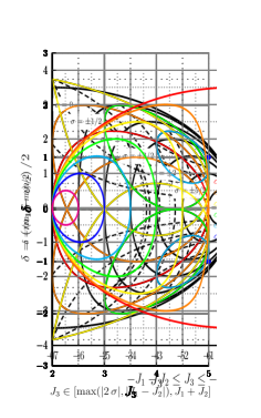
(d) $\sigma=\pm 3/2$

(e) $\sigma=\pm 2$

(f) $\sigma=\pm 5/2$

Figure 1: Caustic and ridge plots (continuous and dashed curves, respectively) of $3j$ symbols for $J_{1}=3/2,J_{2}=7/2$ and for the allowed values of $\sigma$.

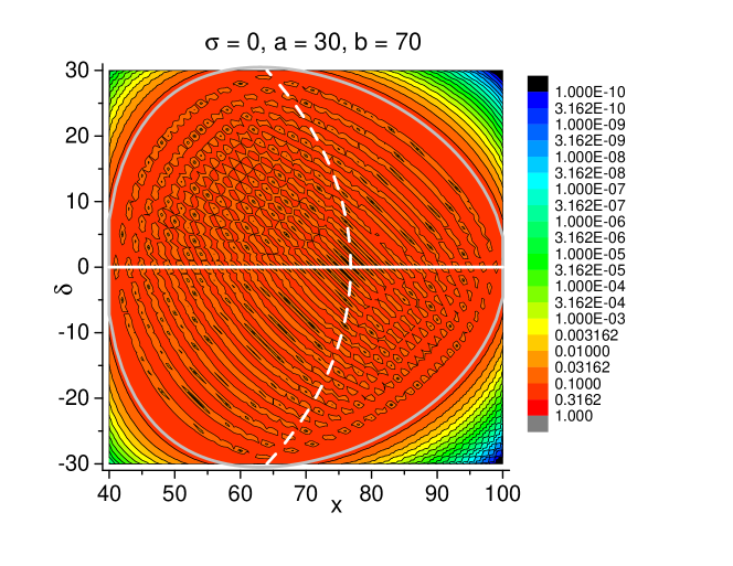
Figure 2: The gray loop is the caustic line, and the dashed and solid white lines are the ridges. The color map log scale plots are for the absolute value of the $3j$ coefficients, and the range is $10^{-10}$ to $1$.

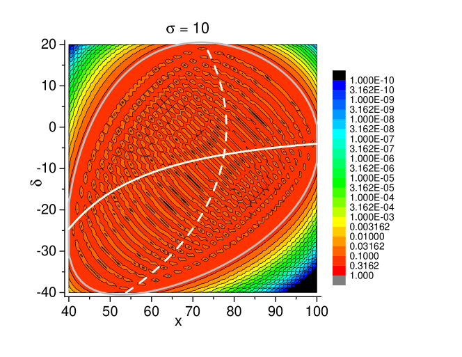
Figure 3: As in Fig. 2 for $\sigma=10$.

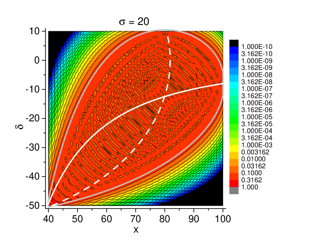
Figure 4: As in Fig. 2 for $\sigma=20$.

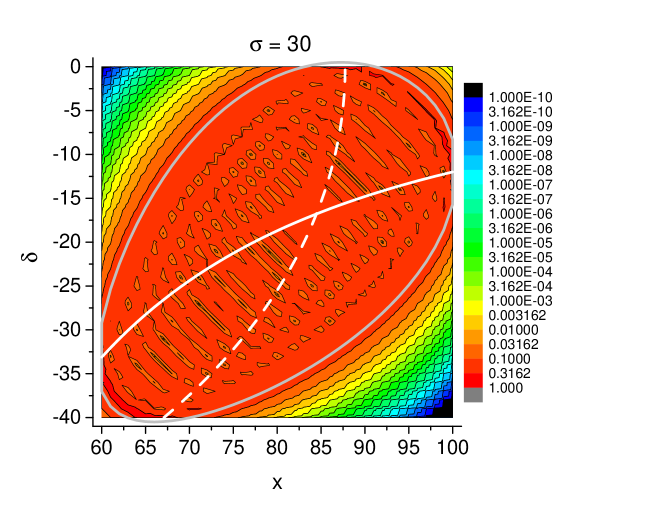
Figure 5: As in Fig. 2 for $\sigma=30$.

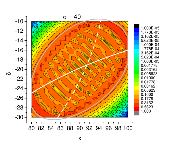
Figure 6: As in Fig. 2 for $\sigma=40$, but with a range from $10^{-5}$ to $1$.

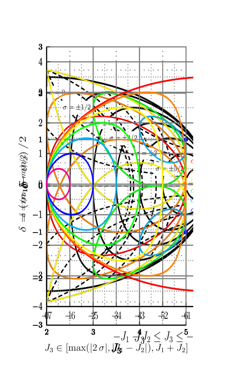
Figure 7: Plots of caustic for $3j$ symbols for $J_{1}=J_{2}=7/2$ and for allowed values of $\sigma$.

7 Concluding remarks

The study of these coefficients is important as orthogonal basis sets in discretization algorithms [22, 25, 26]. In fact, not considered here are their limits to spherical and hyperspherical harmonics (e.g. d matrix) when entries are large. This makes them useful for expanding continuous functions on grids.

An important topics is the semiclassical dynamics associated to the $3j$ symbols, that can be worked out similarly to that for $6j$’s. The interesting geometrical interpretations [27, 28, 29, 30, 31, 32, 33, 34, 23, 35] are also currently being investigated.

8 Appendix: Permutational and “mirror” symmetries

Symbols related by exchange of a column involve a phase change, e.g., in our notation

$$\left(\begin{array}[]{ccc}{a}&{b}&{x}\\ {\alpha}&{\beta}&{\gamma}\end{array}\right)=(-1)^{a+b+x}\left(\begin{array}[]{ccc}{b}&{a}&{x}\\ {\beta}&{\alpha}&{\gamma}\end{array}\right)~{}.$$ (52)

Similarly, changing signs for all projections

$$\left(\begin{array}[]{ccc}{a}&{b}&{x}\\ {\alpha}&{\beta}&{\gamma}\end{array}\right)=(-1)^{a+b+x}\left(\begin{array}[]{ccc}{a}&{b}&{x}\\ {-\alpha}&{-\beta}&{-\gamma}\end{array}\right)~{}.$$ (53)

Substituting our variables, given in Eq. (38), we have

$$\left(\begin{array}[]{ccc}{a}&{b}&{x}\\ {\sigma+\delta}&{\sigma-\delta}&{-2\sigma}\end{array}\right)=(-1)^{a+b+x}\left(\begin{array}[]{ccc}{a}&{b}&{x}\\ {-\sigma-\delta}&{-\sigma+\delta}&{2\sigma}\end{array}\right)~{},$$ (54)

which is used in the screen representation of Sec. 6. The mirror symmetry, i.e. $a\rightarrow-a-1$, $b\rightarrow-b-1$, $x\rightarrow-x-1$ permits the introduction of negative entries, e.g.

$$\left(\begin{array}[]{ccc}{a}&{b}&{x}\\ {\alpha}&{\beta}&{\gamma}\end{array}\right)=(-1)^{b-x-a}\left(\begin{array}[]{ccc}{a}&{b}&{-x-1}\\ {\alpha}&{\beta}&{\gamma}\end{array}\right)$$ (55)

as illustrated in Fig. 8.

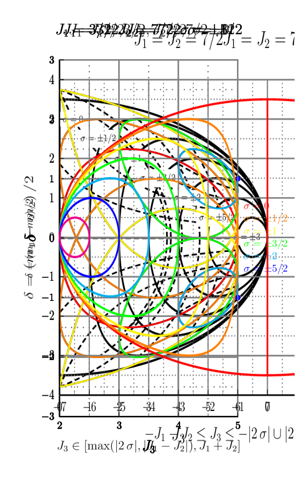
Figure 8: Caustic plots of $3j$ symbols for $J_{1}=J_{2}=7/2$ and for allowed values of $\sigma$.

References

- [1] Zare, R.N.: Angular Momentum. Understanding Spatial Aspects in Chemistry and Physics. Wiley-Interscience, Hoboken (1988)
- [2] Aquilanti, V., Cavalli, S., DeFazio, D.: Angular and Hyperangular Momentum Coupling Coefficients as Hahn Polynomials. J. Phys. Chem. 99(42) (1995) 15694–15698
- [3] Aquilanti, V., Haggard, H.M., Littlejohn, R.G., Yu, L.: Semiclassical analysis of Wigner -symbol. J. Phys. A 40(21) (2007) 5637–5674
- [4] Anderson, R.W., Aquilanti, V., Bitencourt, A.C.P., Marinelli, D., Ragni, M.: The screen representation of spin networks: 2d recurrence, eigenvalue equation for 6j symbols, geometric interpretation and hamiltonian dynamics. Lecture Notes in Computer Science 7972 (2013) 46–59
- [5] Ragni, M., Littlejohn, R.G., Bitencourt, A.C.P., Aquilanti, V., Anderson, R.W.: The screen representation of spin networks. images of symbols and semiclassical features. Lecture Notes in Computer Science 7972 (2013) 60–72
- [6] Bitencourt, A.C., Marzuoli, A., Ragni, M., Anderson, R.W., Aquilanti, V.: Exact and asymptotic computations of elementary spin networks: Classification of the quantum-classical boundaries. In: Lecture Notes in Computer Science. Volume I-7333., Springer (2012) 723–737 See arXiv:1211.4993[math-ph].
- [7] Miller, W.: Classical-limit quantum mechanics and the theory of molecular collisions. Adv. Chem. Phys. 25 (1974) 69–177
- [8] Schulten, K., Gordon, R.: Exact recursive evaluation of 3j- and 6j-coefficients for quantum mechanical coupling of angular momenta. J. Math. Phys. 16 (1975) 1961–1970
- [9] Schulten, K., Gordon, R.: Semiclassical approximations to 3j- and 6j-coefficients for quantum-mechanical coupling of angular momenta. J. Math. Phys. 16 (1975) 1971–1988
- [10] Sprung, D., van Dijk, W., Martorell, J., Criger, D.B.: Asymptotic approximations to Clebsch-Gordan coefficients from a tight-binding model. Am. J. Phys. 77 (2009) 552–561
- [11] Ponzano, G., Regge, T.: Semiclassical limit of Racah coefficients. In Bloch et al., F., ed.: Spectroscopic and group theoretical methods in physics, Amsterdam, North-Holland (1968) 1–58
- [12] Mohanty, Y.: The Regge symmetry is a scissors congruence in hyperbolic space. Algebr. Geom. Topol. 3 (January 2003) 1–31
- [13] Roberts, J.: Classical 6j-symbols and the tetrahedron. Geom. Topol. 3 (March 1999) 21–66
- [14] Aquilanti, V., Marinelli, D., Marzuoli, A.: Hamiltonian dynamics of a quantum of space: hidden symmetries and spectrum of the volume operator, and discrete orthogonal polynomials. arXiv:1301.1949v2 [math-ph], J. Phys. A: Math. Theor. 46 (2013) 175303
- [15] Neville, D.E.: A technique for solving recurrence relations approximately and its application to the 3-J and 6-J symbols. J. Math. Phys. 12(12) (1971) 2438–2453
- [16] Littlejohn, R., Yu, L.: Uniform semiclassical approximation for the Wigner symbol in terms of rotation matrices. J. Phys. Chem. A 113 (2009) 14904–14922
- [17] Biedenharn, L.C., Louck, J.D.: 5.8. Encyclopedia of Mathematics and its Applications. In: Some Interrelations between Angular Momentum Theory and Projective Geometry. 1 edn. Cambridge University Press (1981) 353–369
- [18] Ragni, M., Bitencourt, A., da S. Ferreira, C., Aquilanti, V., Anderson, R., Littlejohn, R.: Exact computation and asymptotic approximation of symbols. illustration of their semiclassical limits. Int. J. Quantum Chem. (110) (2010) 731–742
- [19] Varshalovich, D., Moskalev, A., Khersonskii, V.: Quantum Theory of Angular Momentum. World Scientific, Singapore (1988)
- [20] Neville, D.E.: Volume operator for spin networks with planar or cylindrical symmetry. Phys. Rev. D 73(12) (June 2006) 124004
- [21] Neville, D.E.: Volume operator for singly polarized gravity waves with planar or cylindrical symmetry. Phys. Rev. D 73 (June 2006) 124005
- [22] DeFazio, D., Cavalli, S., Aquilanti, V.: Orthogonal polynomials of a discrete variable as expansion basis sets in quantum mechanics. the hyperquantization algorithm. Int. J. Quantum Chem. (93) (2003) 91–111
- [23] Anderson, R.W., Aquilanti, V., Marzuoli, A.: 3nj Morphogenesis and Semiclassical Disentangling. J. Phys. Chem. A 113(52) (2009) 15106–15117 PMID: 19824616.
- [24] Anderson, R., Aquilanti, V., da S. Ferreira, C.: Exact computation and large angular momentum asymptotics of symbols: semiclassical disentangling of spin-networks. J. Chem. Phys. 129(161101 (5 pages)) (2008)
- [25] Aquilanti, V., Cavalli, S., DeFazio, D.: Hyperquantization algorithm. I. Theory for triatomic systems. J. Chem. Phys. 109(10) (1998) 3792–3804
- [26] Aquilanti, V., Capecchi, G.: Harmonic analysis and discrete polynomials. from semiclassical angular momentum theory to the hyperquantization algorithm. Theor. Chem. Accounts (104) (2000) 183–188
- [27] Marinelli, D., Marzuoli, A., Anderson, R.W., Bitencourt, A.C.P., Ragni, M., Aquilanti, V.: Symmetric angular momentum coupling, the quantum volume operator and the 7-spin network: a computational perspective. Lecture Notes in Computer Science 8579 (2014) 508–521
- [28] Aquilanti, V., Coletti, C.: -symbols and harmonic superposition coefficients: an icosahedral abacus. Chem. Phys. Letters (344) (2001) 601–611
- [29] Chakrabarti, A.: On the coupling of angular momenta. Ann. Inst. H. Poincaré Sect. A 1 (1964) 301–327
- [30] Aquilanti, V., Bitencourt, A., da S. Ferreira, C., Marzuoli, A., Ragni, M.: Combinatorics of angular momentum recoupling theory: spin networks, their asymptotics and applications. Theor. Chem. Acc. 123 (2009) 237–247
- [31] Aquilanti, V., Haggard, H.M., Hedeman, A., Jeevangee, N., Littlejohn, R., Yu, L.: Semiclassical mechanics of the Wigner -symbol. arXiv:1009.2811v2 [math-ph], J. Phys. A 45(065209) (2012)
- [32] Nikiforov, A.F., Suslov, S.K., Uvarov, V.B.: Classical Orthogonal Polynomials of a Discrete Variable (Scientific Computation). Springer-Verlag (10 1991)
- [33] Lévy-Leblond, J.M., Lévy-Nahas, M.: Symmetrical Coupling of Three Angular Momenta. J. Math. Phys. 6(9) (1965) 1372–1380
- [34] Biedenharn, L.C., Louck, J.D.: The Racah–Wigner Algebra in Quantum Theory. Number Rota, G–C. (Ed) in Encyclopedia of Mathematics and its Applications Vol 9. Addison–Wesley Publ. Co.: Reading MA (1981)
- [35] Ragni, M., Bitencourt, A.C.P., Aquilanti, V., Anderson, R.W., Littlejohn, R.G.: Exact computation and asymptotic approximations of symbols: Illustration of their semiclassical limits. Int. J. Quantum Chem. 110(3) (2010) 731–742