Properties of optically selected BL Lac candidates from the SDSS

Abstract

Context. Deep optical surveys open the avenue for find large numbers of BL Lac objects that are hard to identify because they lack the unique properties classifying them as such. While radio or X-ray surveys typically reveal dozens of sources, recent compilations based on optical criteria alone have increased the number of BL Lac candidates considerably. However, these compilations are subject to biases and may contain a substantial number of contaminating sources.

Aims. In this paper we extend our analysis of 182 optically selected BL Lac object candidates from the SDSS with respect to an earlier study. The main goal is to determine the number of bona fide BL Lac objects in this sample.

Methods. We examine their variability characteristics, determine their broad-band radio-UV SEDs, and search for the presence of a host galaxy. In addition we present new optical spectra for 27 targets with improved S/N with respect to the SDSS spectra.

Results. At least 59% of our targets have shown variability between SDSS DR2 and our observations by more than 0.1-0.27 mag depending on the telescope used. A host galaxy was detected in 36% of our targets. The host galaxy type and luminosities are consistent with earlier studies of BL Lac host galaxies. Simple fits to broad-band SEDS for 104 targets of our sample derived synchrotron peak frequencies between $13.5\leq\mathrm{log}_{10}\left(\nu_{\mathrm{peak}}\right)\leq 16$ with a peak at $\mathrm{log}_{10}\sim 14.5$. Our new optical spectra do not reveal any new redshift for any of our objects. Thus the sample contains a large number of bona fide BL Lac objects and seems to contain a substantial fraction of intermediate-frequency peaked BL Lacs.

1 Introduction

Active galactic nuclei (AGN) are compact and extremely luminous objects located in the center of galaxies. They are dominated by a super massive black hole that is continuously fed by infalling gas from the surrounding environment. Their emission is strongly variable and consists of a continuum emission from an accretion disk that dominates the optical to X-ray regime and strong infrared emission that is attributed to a surrounding dusty torus. In addition high-velocity gas is present that manifests itself by emission lines in the optical spectrum. In about 10% of the AGN, synchrotron radiation from a jet dominates, which led to a distinction between radio-loud and radio-quiet AGN. They come in different flavors all of which can well be explained within the so-called “unified scheme” (e.g., Urry & Padovani 1995), where the major difference between each of them is the inclination between the geometry of the system and the line of sight to the observer.

BL Lacertae objects (BL Lacs) are a subclass of AGN characterized by strong variability across the entire electromagnetic spectrum on timescales down to minutes, as well as high and variable polarization. With some exceptions, where narrow emission lines from the AGN itself or absorption lines from their host galaxy are present, their optical spectra are mostly featureless. This is due to strong Doppler-boosting of dominating jet emission, which leads to an outshining of the host galaxy or accretion disk in many cases and to the well-known effect of superluminal motion. Within the unified scheme, BL Lacs are thought to be Fanaroff-Riley class I radio galaxies (Fanaroff & Riley 1974), whose jets are aligned within a few degrees to the line of sight. Not surprisingly, they are rare. In the latest AGN catalog of Véron-Cetty & Véron (2010), fewer than $1\%$ objects are listed as BL Lacs.

Although apparently simple, there has been an intense discussion of the defining characteristics of a BL Lac since their detection. For example, Stickel et al. (1991) classified objects as a BL Lac when their optical spectrum did not contain lines with a rest-frame equivalent width (RFEW) exceeding 5Å, while Stocke et al. (1991)) used the criteria of synchrotron emission dominating the optical spectrum, as well as optical (variable) polarization. The former criterion was violated at least once by the prototype BL Lac itself (Vermeulen et al. 1995). For a long time it is known that the properties of a given BL Lac sample are depending on the selection frequency. Early BL Lac samples were formed by identifying the optical counterparts of radio (Stickel et al. 1991) or X-ray (Perlman et al. 1996) sources and finding targets with featureless optical spectra. The former method favored BL Lacs with synchrotron peaks in the infrared range, while the latter favors targets with their synchrotron emission peaking in the UV to X-ray regime, leading to an apparent bimodality in source properties when viewed in the $\alpha_{ox}$ - $\alpha_{ro}$ plane (e.g., Padovani & Giommi 1995). Later surveys employing cross-correlations between radio and x-ray surveys (Laurent-Muehleisen et al. 1999; Giommi et al. 2005) have found intermediate targets filling the gap, but even these samples may be biased by the shallowness of the respective surveys and do not give the full picture of the BL Lac population. Nowadays, it is clear that the distribution of synchrotron peak frequencies is not bimodal (e.g., Abdo et al. 2010), also resulting in continuous coverage in the $\alpha_{ox}$ - $\alpha_{ro}$ plane. BL Lacs are commonly dubbed as low-frequency peaked (LBL), intermediate-frequency peaked (IBL), and high-frequency peaked (HBL) BL Lacs depending on the frequency of the synchrotron peak $\nu_{peak}$. Given the continuous distribution of $\nu_{peak}$, the limits for different classes are somewhat arbitrary. In this paper we use the common convention to classify a BL Lac as an LBL if $\log{\nu_{peak}}<14$, IBL if $14\leq\log{\nu_{peak}}<15$, and HBL if $\log{\nu_{peak}}\geq 15$.

With the advent of large optical surveys (such as SDSS), it became possible to obtain samples that potentially populate the IBL region and may be more representative of the BL Lac class as a whole. Collinge et al. (2005) (C05 hereafter) extracted a sample of 240 probable BL Lac candidates from the SDSS survey DR2 (York et al. 2000) in order to find an IBL sample not biased by X-ray or radio properties (see note 1 in Heidt & Nilsson (2011), hereafter Paper I). A more recent selection, albeit with a slightly different approach, was presented by Plotkin et al. (2010). They recovered the majority of candidates found by C05 and enlarged the probable candidate list to over 700 objects using SDSS DR7. Despite the careful selection process, possible confusion by stellar (e.g., DC white dwarfs, see Angel 1978) or extragalactic (e.g., weak-lined quasars, see Fan et al. 1999) sources may be present and cannot be ruled out without further observations.

In Paper I we presented the polarization properties of 182/204 BL Lac candidates from C05. We found 124 out of 182 targets (68%) to be polarized and 95 of the polarized targets (77%) to be highly polarized ($>$ 4%). This indicates that the C05 sample of probable BL Lac objects indeed contains a large number of bona fide BL Lacs.

With the present paper we enlarge our study of the properties of this sample. Using our polarimetric data in combination with the SDSS measurements, we look for optical variability and study the host galaxy properties of our 182 objects. In addition, using the data available in the literature, we constructed broad-band spectral energy distributions (SEDs). They are used to fit simple synchrotron models to them in order to derive peak frequencies and to determine their LBL/IBL/HBL nature. Finally, new optical spectra for 27/182 objects are presented. In section 2 we briefly summarize the resources used for our data extraction followed by a description of the analysis in section 3. The results are discussed in section 4 and summarize in section 5. For a detailed discussion of the global properties of our sample, a comparison to other samples and a potential revision of the defining criterion of a BL Lac, we refer to Paper III (Nilsson et al., in prep).

Throughout this paper we use standard cosmology ($H_{0}=70$ km s^-1 Mpc^-1, $\Omega_{M}$ = 0.3, and $\Omega_{\Lambda}$ = 0.7). When discussing the results of a K-S test, we denote two distributions that are significantly different if the null hypothesis that they are drawn from the same parent population can be rejected with p $<$ 1%.

2 Data acquisition and reduction

2.1 Variability and host galaxies

The data that we use for variability and host galaxy analysis were presented in Paper I, where a detailed log of the observations can be found. Here we briefly repeat the main characteristics of the observations.

Alltogether, 123 targets were observed at the ESO New Technology Telescope (NTT) on La Silla, Chile during Oct. 2-6, 2008 and Mar. 28 - Apr. 1, 2009. The observations were made with the EFOSC2 instrument through a Gunn-r filter (#786). We used a 2k Loral chip with a gain of 0.91 e${}^{-}/$ADU, readout noise of 7.8 e^- and pixel scale of 0$\aas@@fstack{\prime\prime}$24/pixel in 2x2 binning mode. The total field of view was 4’$\times$4’. The observations were made in polarimetric mode; i.e., a Wollaston prism and a half-wave plate were inserted into the beam, resulting in two images of each target on the CCD, separated by 10 ″. One polarization observation consisted of four exposures of 10-1000s each at different polarization angles (0, 22.5, 45, and 67.5 degrees) of the half-wave plate, resulting in eight images per target per polarization observation. In most cases a single sequence was obtained, but two to three sequences were made for fainter targets. Seeing was generally good (0$\aas@@fstack{\prime\prime}$6-1$\aas@@fstack{\prime\prime}$2) during the NTT runs and the weather was photometric, except for the last half night of NTT run in March, when thin clouds increasingly covered the sky toward the morning.

Another set of 47 targets was observed in service mode at the Calar Alto (CA) 2.2 m telescope using the CAFOS instrument on Feb. 18-24, 2009. The observations were made through a Gunn-r filter using the central 1000$\times$1000 pixels of the Site-CCD with a gain of 2.3 e^-/ADU, readout noise of 5.1 e^-, and pixel scale of 0$\aas@@fstack{\prime\prime}$51/pixel, resulting in a field of view of 7’$\times$7’. The observations were made using a polarimetric setup similar to the NTT, except that the separation of the images was 19″. Exposure times varied from 30 to 1000 s per half-wave plate position. Seeing was better than 1$\aas@@fstack{\prime\prime}$5 throughout the run and weather was photometric.

Finally, 25 objects were observed using the ALFOSC instrument at the Nordic Optical Telescope (NOT). Observations were made through the SDSS-r’ (#84) filter using the central 1500$\times$650 pixels of an E2V-CCD with a gain of 0.736 e^-/ADU, readout noise of 5.3 e^-, and pixel scale of 0$\aas@@fstack{\prime\prime}$19/pixel, giving a field of view of 4$\aas@@fstack{\prime}$7$\times$2’. A similar polarimetric mode was used here also, except that a calcite plate was inserted into the beam to provide a beam separation of 15″. Exposure times varied from 150 to 1000 s per half-wave plate position. Seeing varied between 0$\aas@@fstack{\prime\prime}$7-1$\aas@@fstack{\prime\prime}$5, and the weather was mostly photometric throughout the run, except for some low-altitude cirrus on the last of the three nights.

All in all, we have 195 observations of 182 targets, i.e. 13 targets were observed twice. The images were reduced by first subtracting the bias frame and then were divided the frames by a flat-field, which was obtained either from the twilight sky (NTT and NOT) of from an evenly illuminated screen inside the dome (CA). Dark current was negligible in all cases.

2.2 Optical photometry (SDSS)

For estimating the zero points of the various science fields, the photometry performed by the Sloan Digital Sky Survey (SDSS) Data Release 2 (Abazajian et al. 2004) was used. The SDSS is the deepest and most complete optical survey to use a dedicated 2.5m telescope at the Apache Point observatory. A detailed description of the instrument can be found in Gunn et al. (1998).

2.3 Optical spectra

Using the analysis of Paper I, candidates with unknown redshift and high polarization ($>$4%) were targeted for spectroscopy. In total 27 of 87 targets fulfilling this requirement were observed. The observations were performed at the Calar Alto 2.2 m telescope during eight nights between March 17 and April 27, 2011. We used the CAFOS instrument in the long-slit mode with the G-200 grism (Nr.9) and a slit with of 2-3″(10″for standards). With the chosen grism, the spectral range was from 440 to 850 nm with a resolution of $\lambda/\Delta\lambda\approx 400$ at 500 nm. Every night at least one spectrophotometric standard star (Hiltner102, HZ44, BD+33$\_$2642) was observed, and a continuum lamp flat field and an arc exposure was made after every observation. In order to reach a high S/N ratio and to be able to correct for cosmic ray hits, three 2400 s exposures were taken for each object.

The spectra were reduced by subtracting the average bias images taken at the beginning and at the end of each night. Then every image was divided by its adjacent bias-subtracted flat using standard IRAF tasks. The deflection of the spectrum perpendicular to the dispersion axis (centroid shift) was fitted by a third-order polynomial. After background determination and subtraction the spectra were extracted using an appropriate aperture. The spectra were then wavelength-calibrated using the arc-lamp-spectra and the night-sky and finally flux-calibrated using the standard star observed the same night.

2.4 Data for SED fits

To construct broad-band SEDs we used archival data from FIRST (Faint Images of the Radio Sky at Twenty-Centimeters, Becker et al. 1995), the NVSS (NRAO VLA Sky Survey, Condon et al. 1998), WISE (Wide-Field Infrared Survey Explorer, Wright et al. 2010), UKIDSS (the United Kingdom Infrared Deep Sky Survey DR9, Lawrence et al. 2007), the SDSS (Sloan Digital Sky Survey DR5, Adelman-McCarthy et al. 2007), GALEX (Galaxy Evolution Explorer, Martin et al. 2005), and the RASS (ROSAT All Sky Survey, Voges et al. 2000). Some more data points were derived using the NED (NASA extragalactic database - http://ned.ipac.caltech.edu/). Broad-band SEDs could be retrieved for 104 out of our 182 objects.

3 Analysis

3.1 Flux calibration

We used the data set from Paper I for the test of variability and for the host galaxy study. Both studies require accurate photometric calibration of the frames, which we describe in this section. For the flux calibration we used stars on the CCD frames with SDSS r-band modelMag magnitudes and $g-r$ colors available from the SDSS DR2. Each observing run, NTT March, NTT October, NOT, CA was calibrated as a separate block with the exception of NTT March, where the last night of this observing run was treated separately due to increasing cloud coverage toward the end of the night. The rest of the data were obtained in photometric conditions.

Figure 1: Transmission curves of the filters used for our observations together with the SDSS r-band filter.

Since our filter band-passes differ from the SDSS r-band (Fig. 1), a color dependence in the calibration is expected. Furthermore, the spectra of the BL Lac nuclei are dominated by a power-law continuum, which differs significantly from the spectra of the stars used for calibration, whereas the host galaxies have a SED closer to the stars. Based on these considerations we used two different equations for the calibration, one for the stars and host galaxies and another for the BL Lac nuclei. The general form of this equation can be written as

$$r=\overline{K_{0}}-2.5\log N+C$$ (1)

where $r$ is the SDSS r-band magnitude, $\overline{K_{0}}$ the magnitude zero point of the run, $N$ the measured counts/s from the target (ADU/s), and $C$ a color-correction term. For the stellar/host galaxy correction we used a linear color correction $C=s\cdot(g-r)$ with $s$ the slope. The color correction for the active nucleus that is color-independent constant which will be discussed extensively in the Section 3.2. The linear equation was fit to each run separately to obtain $\overline{K_{0}}$ and $s$. The count rate $N$ for each star was determined by performing aperture photometry to all eight images in the polarization sequence, thus eliminating the modulation by the polarization optics. We did not correct for atmospheric absorption since the average absorption is included in $\overline{K_{0}}$, and the RMS scatter of the zero points $K_{0}$ of individual images is much higher than the extinction by the atmosphere; i.e., no dependence of the zero point as a function of airmass was found.

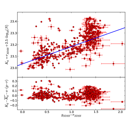
Figure 2: Upper panel: The linear dependence of the ZP as function of the SDSS color (for 412 stars) for Calar Alto data. The vertical branch at $g-r>1.3$ is discussed in the text. The blue line is the fitted behavior found by minimizing $\chi^{2}$. Lower panel: The color dependence after subtraction of a linear dependence.

Figure 2 shows an example of the color dependence in the data. There is an approximately linear dependence of $K_{0}=r+2.5\log N$ on the color of the star. Two things are apparent in this plot: some stars reside significantly below or above the main body of the data, and there is a conspicuous clustering of points in the upper righthand corner of the plot. The former property is probably due to measurement errors and variability of the stars. The second property, present in all but the NOT data, resides approximately at $g-r>1.3$, which corresponds to stars with temperatures of less than $\sim 3500$K, indicating that the branch is mainly populated by M dwarfs and red giants. While M dwarfs show a more or less linear color dependence in the optical (Allard & Hauschildt 1995), red giants show broad absorption bands in the SDSS r-band (Johnson et al. 1980), leading to an increase of $r$ (decrease of $g-r$). Since the depth of the absorption band increases with decreasing temperature (increasing $g-r$), the color $g-r$ only weakly depends on the temperature, so that colder giants (down to $\sim 2000$K) reside in the same color range. This explains the vertical structure of the color plot in an excellent way. The reason for not seeing the vertical branch in the NOT data set is obviously that nearly identical filters were used, and furthermore the small number statistics of calibration objects, due to the small FOV, prohibits the detection of such a possible branch (called red branch hereafter).

To exclude extreme outliers and to get rid of highly variable stars, we subsequently performed a Kappa-Sigma clipping of the data. We first fitted the color dependence with a linear dependence and subtracted the fit from the data. Then we computed the standard deviation of the residuals and clipped away the most extreme outsiders (threshold $\sim 3\sigma$). This clipping was iterated twice to obtain the final fit. The fit was then subtracted from the individual $K_{0}$’s and a histogram of the residuals created. To this histogram, a Gaussian distribution is fitted by minimizing $\chi^{2}$. The center of the distribution is then the $\overline{K_{0}}$ and the Gaussian width of the distribution $\sigma_{K_{0}}$ its error.

At this point the red branch introduces another problem. The clustering of points at $g-r>1.3$ may bias the fitted $s$ value upward, resulting in a double-peaked or skewed Gaussian distribution of the residuals. Thus another possibility for fitting the color dependence is to minimize the width of the resulting histogram by iteratively fitting different lines to the color dependence and fitting a Gaussian to the resulting residual distribution. Fortunately only for the NTT(Oct) run does the branch have a significant effect on the resulting distribution. For these data the difference in the slopes $s_{\sigma}$, obtained by minimizing the width of the Gaussian and $s_{\chi^{2}}$, obtained by minimizing the $\chi^{2}$ in the ZP-color plot, is treated as an additional error (see below for details). The fitted color terms $s$ can be found in Table 1.

3.2 Variability

After performing the calibration we measured the target brightnesses by aperture photometry in a similar way to the calibration stars. The light from disturbing adjacent objects was subtracted if there was any leakage into the aperture. Since the total flux of our targets is a sum of two components, the AGN nucleus and the host galaxy, with the former definitely exhibiting a non-stellar spectrum, the color term $C=s\cdot(g-r)$ in Eq. 1 derived from stars is valid only for host-galaxy-dominated targets. A different $C$ should in principle be used for power-law dominated targets.

Table 1: Computed parameters for testing variability.

Parameter	NTT(Mar)		NTT	CA	NOT
	N 1-3	N 4	(Oct)
# calibrators	344	220	306	412	40
s	0.14	0.14	0.14	0.15	-0.003
$C_{AGN}$	0.10	0.10	0.10	0.09	0.02
$\sigma_{K_{0}}$	0.023	0.053	0.027	0.062	0.038
$\sigma_{c}$	0.019	0.014	0.038	0.034	0.001
$\langle VL\rangle$	0.101	0.182	0.208	0.275	0.152

To estimate the color correction for power-law-dominated targets, denoted $C_{AGN}$ here, we created a power-law spectrum with spectral slope of $\alpha_{\nu}=1.16$ $(F_{\nu}\propto\nu^{-\alpha})$, which is typical of optically selected BL Lac candidates (Plotkin et al. 2010), and used synthetic photometry with the SDSS r-band filter bandpass curve and the NTT, CA, and NOT filter band passes to derive $C_{AGN}$. The derived color-correction values $C_{AGN}$ can be seen in Table 1. From this table we see that the color correction for power-law dominated targets is not very different from stellar targets. A power-law index of $\alpha_{\nu}=1.16$ corresponds to g - r = 0.36, for which the stellar color correction is $\sim 0.05$ mag in the case of the NTT and CA data.

Since the total light from our targets is a superposition of two components, the power-law nucleus and the host galaxy with a stellar-type spectrum, the SDSS r-band magnitude can be calculated from our data only if the power-law slope and the host galaxy fraction are known precisely. As described in the next section, we were able to resolve the host galaxy in only about one third of the targets, so even though the host galaxy fraction is known for a significant part of our sample, it is uncertain for the major part. Additionally, the power-law index of the optical nucleus is uncertain for most of the targets. Because of these uncertainties and in order to treat the whole sample homogeneously, we treated the entire sample statistically using an average $\alpha_{nu}$ and nucleus/host galaxy ratio. This obviously introduces errors to the derived r-band magnitudes, and we propagated this error into the final magnitude errors as described below.

Based on the discussion above, the SDSS r-band magnitudes were computed as follows. We first computed the average of the two extreme color corrections (pure AGN and pure host galaxy), averaged over each run:

$$\langle C\rangle=\frac{1}{N}\sum\limits_{i=1}^{N}\leavevmode\nobreak\ \left(\frac{s\cdot(g-r)+C_{AGN}}{2}\right)=\frac{1}{N}\sum\limits_{i=1}^{N}\leavevmode\nobreak\ C_{i}\ ,$$ (2)

where $N$ is the number of targets in the run. The $\langle C\rangle$ gives the typical correction between the two SEDs (stellar and power law) through the different filters used. This value is then added to the “raw” magnitude (Eq. 1 without color correction), and the RMS scatter of this quantity, $\sigma_{C}$ is treated as the error of our color correction. This RMS scatter depends on the sample and even on color in the case of NTT(Oct), for the reasons explained below.

An object is called variable if the difference between our magnitude and the SDSS magnitude, hereafter called variability amplitude, is greater than the variation limit $VL$, which is computed by

$$VL=3\sqrt{\sigma_{K_{0}}^{2}+\sigma_{C}^{2}+\sigma_{SDSS}^{2}+\sigma_{phot}^{2}}\ ,$$ (3)

where $\sigma_{K_{0}}$ and $\sigma_{C}$ have been discussed above and $\sigma_{SDSS}$ and $\sigma_{phot}$ are the photometry errors of the SDSS and our data, respectively. The errors of the SDSS and our photometry are generally small compared to $\sigma_{K_{0}}$ and $\sigma_{C}$.

Slight adjustments to this scheme were made owing to complications in the data. To compensate for the clouds in the second half of the fourth night of the NTT March run, the $K_{0}$ of each image was derived, and a correction due to clouds was computed using the average $K_{0}$ of the first half of the night. Even though this was done for each image individually, the overall distribution of $K_{0}$ of the fourth night was broadened significantly so that we decided to evaluate the last night separately.

For the NTT October data, the red giant branch had such a strong influence on the resulting standard deviation of the Gaussian distribution that the $\chi^{2}$ fit could not be applied to fit the color dependence. The difference in the color term $s$ between the $\chi^{2}$ ($s_{\chi^{2}}$) and the ”best Gauss” fit ($s_{\sigma}$) was added as an additional (color-dependent) error to the variation limit:

$$VL^{2}_{NTT(Oct)}=VL^{2}+\left[\left(s_{\chi^{2}}-s_{\sigma}\right)\left(g-r\right)_{S}\right]^{2}\,\,.$$ (4)

This additional error affected the variation statement of only two objects. The CA data also showed a rather extreme red branch, but owing the broadening of the distribution to the smaller primary mirror, the effect was negligible so that $s_{\chi^{2}}\approx s_{\sigma}$. Because of the small mirror and the use of the Gunn r filter, the CA data resulted in the worst sensitivity for testing variability.

The NOT data set was affected by a very small FOV so that the number of calibration objects was very low. Of the 59 chosen objects, 19 were cut away by the two clippings, resulting in a Gaussian plot with fairly low number statistics, so instead of employing a Gaussian fit to the data, we used the standard deviation of the ZP distribution to estimate $\sigma_{K_{0}}$. The NOT data benefit from the available filter, which is nearly identical with the SDSS r-band, causing the color correction for calibration stars and BL Lac candidates to be very small. This shows the importance of the choice of the filter since the only parameters affecting the precision of the photometry, in addition to photometric errors and clouds, is the collecting area of the telescope. We therefore would expect a much higher precision at NTT, which was frustrated by the color correction.

For four objects no statement of variability could be made as those showed such extreme spectra that our color correction cannot yield reliable results. For instance, in SDSS J004054.65-091526.8, the Ly$\alpha$ edge lies exactly between the Gunn r and the SDSS-r filter. These objects were excluded from the variability analysis.

3.3 Host galaxies

The host galaxy analysis was performed with the model fitting software we have used extensively during our previous studies of BL Lac host galaxies (e.g. Heidt et al. 1999; Nilsson et al. 2003, 2007). A more detailed description of the fitting procedure can be found in Nilsson et al. (1999), here we briefly describe the main features of the program and its application to present data.

Polarimetric imaging differs from conventional imaging in a few important aspects. Firstly, each target produces two images on the CCD corresponding to the two orthogonally polarized beams (see Fig. 3). In our case the beams were separated vertically by 10-19″on the CCD depending on the instrument. Secondly, the intensity of polarized targets is modulated by the position angle of the half-wave plate, and therefore some BL Lacs exhibit varying peak intensity in both beams over the four image polarimetric cycles. Furthermore, since the two beams go through different optical paths, the PSF shapes of the two images are different from each other. The first property means that great care must be exercised to identify and mask out overlapping images from nearby targets. Furthermore, if the diameter of the target is larger than the beam separation, the two images start to overlap, which must be taken into account in the analysis. The second property can be circumvented by summing the four images of the polarimetric cycle, which effectively removes the modulation. The third property does not cause problems if an empirical PSF (i.e., a PSF derived from field stars) is used.

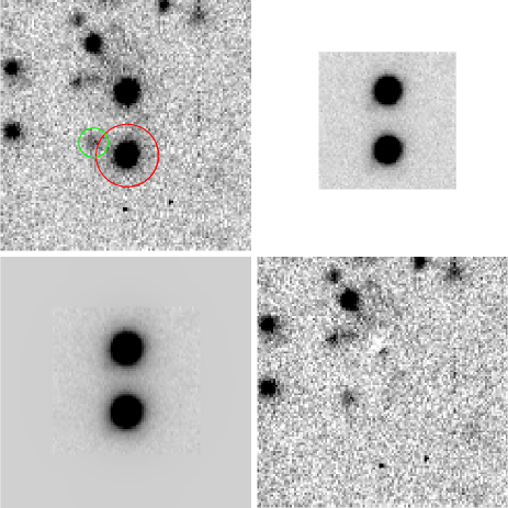
Figure 3: Upper left panel: Gunn r-band image of SDSS J215051.73+111916.6 obtained at the NTT. Note the double image of the target created by the polarization optics. Field size is 29$\times$29″, north is up and east to the left. The red circle marks the area included in the fit and the green circle an area masked out due to an overlapping target. Upper right panel: PSF image extracted from a field star. Lower left panel: Best fit model (core + host galaxy) of the target. Lower right panel: Residuals after subtracting the model.

The model fitted to the observed images consists of two components, the unresolved core, parameterized by position $x_{c}$,$y_{c}$ and magnitude $m_{c}$, and the host galaxy parameterized by position $x_{g}$,$y_{g}$, magnitude $m_{g}$, effective (half-light) radius $r_{e}$, ellipticity $\epsilon_{g}$, and position angle of the host galaxy $\theta_{g}$. The ellipticity and position angle were free parameters only for well-resolved targets and were fixed at 0.0 for the rest. To test for host galaxy type, we fitted two different host galaxy models: a bulge model represented by deVaucouleurs profile with $\beta=0.25$ and a disk model with $\beta=1.0$, where $\beta$ is the profile slope in

$$I(r)=I(r_{e})\ {\rm dex}\left\{-b_{\beta}\left[\left(\frac{r}{r_{e}}\right)^{\beta}-1\right]\right\}\ ,$$ (5)

where $b_{\beta}$ is a $\beta$-dependent constant so that $r_{e}$ always encircles half the host galaxy light. The model fit was made using an iterative Levenberg-Marquardt loop, which finds the set of parameters minimizing the chi squared between the data and the model.

The model was convolved with the PSF, which was obtained from a suitably bright field star. We first tried the fit using both images simultaneously; i.e., the PSF consisted of a double image of a field star, and both target images were used for the fit. This has the advantage that even cases where the two images partly overlap can be fit accurately since the overlap is included in the model. However, our simulations (see below) showed that the results are sometimes very noisy in this case since the distance between the two images was not constant over the field of view, leaving strong residuals after the fit. The other disadvantage was that a PSF that consists of both images of a star includes lots of pure sky, especially at the CA and NOT where image separation was large, resulting in noisier PSF scaling and consequently noisier results. We thus decided to only use one of the images for fitting, the one with fewer overlapping targets and/or rounder PSFs. This effectively means sacrificing half of the signal for better fitting results and simplified error analysis.

The fitting procedure thus progressed as follows. First all 4 to 12 images in the polarimetric sequence were summed, and of the two target images on the CCD, the one better suited to fitting was selected. All overlapping targets were masked out and the background was subtracted by measuring 4 to 8 sky regions around the target. Next, a suitable PSF star was selected and extracted. For the NTT images we extracted a “double” PSF, but used only one of the PSF images for fitting. This enabled us to model any leakage from one component of the double image to the other. For the CA and NOT images, only the half of the PSF corresponding to the selected target image was extracted. In the few cases where the two images overlapped, we took great care to mask the regions affected by the overlap. In most cases, however, the two images were clearly separated, and as stated above, for the 123 NTT images the overlap was included in the model, so image overlap had no major effect on our results. Next we fitted the image with a model consisting of only the core component; i.e., the fit had three free parameters, $x_{c}$, $y_{c}$, and $m_{c}$. If the residuals showed any hint of a host galaxy, we continued by fitting the $\beta=0.25$ and $\beta=1.0$ models to the observed image. During these fits the position of the core and host galaxy were held constant at the values obtained from the pure core fit and $m_{c}$, $m_{g}$, and $r_{e}$ (and $\epsilon_{g}$ and $\theta_{g}$ for the largest targets) were allowed to change freely.

Calibration of the data was made using Eq. 1 and $C=s\cdot(g-r)$ for host galaxies and the $C_{AGN}$ values in Tab. 1 for the AGN. The redshift-dependent $g-r$ color of the host galaxies was taken from Fukugita et al. (1995) using the curve for elliptical galaxies. For the galaxies with no z, we used z = 0.5.

In addition to the model fits, we performed Monte Carlo simulations to determine the errors of fitted parameters, to decide if a host galaxy was detected and to determine if one of the host galaxy models (bulge or disk) is clearly preferred. We created 100 simulated images of each target corresponding to the best-fit parameters and including properly scaled photon and readout noise, sky determination error, and PSF variability and performed the fits on the simulated images in exactly the same way as for the real images. The PSF variability was introduced by producing two slightly different PSFs for each simulation. The first PSF was used to convolve the simulated model, and the second PSF was used in the fit as the PSF model. Both PSFs were represented by a Moffat profile, but they differed with respect to their ellipticity and position angle by an amount that quantitatively reproduced the peak-to-peak residuals seen in the data. All fits on simulated images were made keeping $\beta$ constant at 0.25 or 1.0, depending on which model was preferred by the actual fit on the data. However, the $\beta$ value for the simulated host galaxy was drawn from a Gaussian distribution with average 0.25 or 1.0 and 10% standard deviation to simulate the natural variability of galaxy profiles.

After the simulations we computed the standard deviations $\sigma$ of the fitted parameters. To consider the host galaxy detected, we required that $\sigma_{m_{g}}$ is $<0.3$. Furthermore, we considered that the host galaxy type was determined if the chi squared value of one model (e.g. bulge) was significantly better than the other (disk), significantly meaning that $|\chi^{2}_{bulge}-\chi^{2}_{disk}|<3\ \sigma_{\chi^{2}}$, where $\sigma_{\chi^{2}}$ is the standard deviation of the chi squared in the simulations.

3.4 Optical spectra

After inspecting all spectra for cosmic ray hits and correcting by interpolation, the S/N ratio of the individual spectra was determined (cf. Table 4). This was found to be 50% higher on average than in the SDSS spectra, as expected from comparable mirror sizes and an exposure time at least a factor of two higher. All possible absorption and emission features were tested individually for their reliability. Any feature was deemed reliable if it was present in at least two thirds of the individual spectra 10$\sigma$ above the background, or in all three spectra 5$\sigma$ above the background. The confirmed spectral features were then compared to the most prominent features typically seen in BL Lacs surrounded by an elliptical galaxy in order to determine a redshift.

3.5 Broad-band SEDs

One powerful tool for separating BL Lac objects, say from thermal sources, is the inspection of their broad-band SED. In AGN, the distribution is a superposition of thermal emission from the accretion disk (power-law with exponential drop-off), a thermal component from the dusty torus, and synchrotron emission from a jet, as well as host galaxy emission, while for thermal sources (e.g., stars) the spectrum is dominated by blackbody emission in the NIR-UV range alone. BL Lacs should be entirely dominated by synchrotron emission at low frequencies and synchrotron-self-Compton processes at higher frequencies. Since the flux spans a range of five orders of magnitude, with variability across all bands, the errors of the fluxes, as well as non-simultaneity were not taken into account for the SED fits. Once the SEDs are fitted and a peak frequency is obtained, their rest-frame frequencies are derived using the spectroscopic redshift (including uncertain ones) given by SDSS. The surveys, along with the bands and their central wavelengths, are listed in Table 2.

Table 2: Surveys used for extracting of the SEDs.

Survey	Band	$\mathrm{log}_{10}\left(\nu_{\mathrm{cen}}\right)$
ROSAT	1.2 - 2.0 keV	17.512
GALEX	NUV	15.115
	FUV	15.287
	u	14.928
	g	14.800
SDSS	r	14.683
	i	14.595
	z	14.521
UKIDSS	y	14.468
	J	14.380
	H	14.265
	K	14.135
	W1	13.946
WISE	W2	13.814
	W3	13.398
FIRST/NVSS	1.42GHz	9.152

The magnitudes are converted to spectral fluxes (Jy) using the standard zero points. For FIRST, NVSS, and GALEX, they are already tabulated in Jy, while for WISE, UKIDSS, and SDSS, we used the conversion given in Wright et al. (2010), Hewett et al. (2006), and Fukugita et al. (1996), respectively. The ROSAT fluxes are given in $erg/cm^{2}/s$ and are converted to Jy by

$$F_{\nu}[Jy]=F[erg/cm^{2}/s]\cdot 10^{23}/\nu_{\mathrm{cen}}[\mathrm{Hz}]\,.$$

The spectral fluxes are then multiplied with the frequency to obtain flux-energy densities.

To derive peak frequencies we did not fit a full synchrotron model starting from a given electron distribution. Instead, we followed the approach by Nieppola et al. (2008) and applied a second-order polynomial to the data in log-log space. This avoids over-fitting of the mostly poorly populated SEDs by tuning too many free parameters.

In addition, we did not include the ROSAT data in our fits since we are only interested in the peak frequency of the synchrotron emission . Moreover, flux densities at keV energies are available for only a few objects and are completely absent at higher frequencies. On the other hand, the X-ray data at least allow the reliability of a fit to be judged.

Because we are fitting global SEDs, we restrict ourselves further to objects where measurements in at least 12 bands are available. Since our measurements are heavily skewed toward IR-optical frequencies, we separate our fits into three categories. Fits to objects with fewer than two radio data points are flagged “Uncertain”. If the number of radio data points exceeds two, but the total number of SED points is less than 14, the objects are flagged “OK”, and the rest of the objects are flagged as “Good”.

The SED fits for each object are displayed in the Appendix (A). The fits give a good indication of the peak frequency for most of the objects, even though the fits are not satisfactory for some of the SEDs, for the reasons mentioned above. For three targets, we derived unreasonably high peak frequencies ($\mathrm{log10}\left(\nu_{peak}\right)>30$). They were not taken into account any further but are shown for completeness. The reliability of the SED fits for targets with only one or no radio data point is somewhat questionable since the low-frequency part of the SED is strongly underpopulated here. Also targets where the host galaxy contribution outweighs the flux originating in the nucleus (i.e., core fraction $<$ 0.5) should be considered as rather uncertain.

4 Results

4.1 Variability

After evaluating all the objects described above, 107 of the 182 targets (59%) showed variations according to our definition. Of the 13 objects measured at two different epochs, two showed variations at one epoch but no variability in the other with respect to the SDSS photometry. This is likely to be partly due to the lower sensitivity of the CA data and partly due to our inability to detect variability using very few data points, so both objects were marked as variable. The distribution of variability amplitudes in Fig. 4 shows that extreme variations up to 2 mag occur, but they are very rare, and most objects vary within the range of 0.2-0.4 mag.

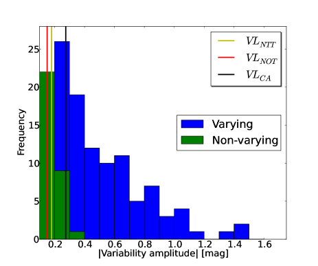
Figure 4: Histogram of variability amplitudes.

We checked to what extent the above result depends on observational errors by creating 1000 mock samples of 178 targets (182 minus the 4 targets with complex spectra). Simulated magnitudes for both the SDSS and our photometry were drawn from a Gaussian distribution with a mean corresponding to the observed value and $\sigma=\sigma_{SDSS}$ for the simulated SDSS magnitudes and $\sigma=\sqrt{\sigma_{K_{0}}^{2}+\sigma_{C}^{2}+\sigma_{phot}^{2}}$ for simulated photometry of this paper. We also included the additional error due to the red branch in the simulation and that 13 targets were observed twice by us. We then classified the targets into variable and non-variable using the same criteria as for the real data and computed $N_{var}$, the number of variable targets. The resulting distribution of $N_{var}$ is close to Gaussian with the center at $N_{var}$ = 108.8 and $\sigma=3.4$. The 3$\sigma$ confidence interval of $N_{var}$ is thus (99,119), meaning that up to 8 targets marked as variable in our sample could be non variable in reality. On the other hand, we may have failed to detect variability in up to 12 targets. These numbers do not take into account the very sparse sampling. Having more sampling points would increase $N_{var}$, so our fraction of variable targets should be considered a lower limit.

The correlation between polarization discussed in Paper I and variability amplitude is shown in Fig. 5. Out of the 107 variable objects, 83 ($78\%$) are polarized as well. The polarization fraction of non-variable objects is significantly lower ($<55\%$), but neither a K-S test nor a linear regression fitted to the variability-polarization plane with subsequent Kappa-Sigma-clipping yielded any correlation between polarization and variability. Since we are comparing an absolute (one-epoch) to a relative (two-epoch) measurement, we do not expect to see any simple correlation.

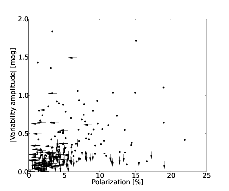
Figure 5: Polarization versus variability amplitude.

Out of the 107 varying objects, only 37 ($35\%$) have a secure redshift while further 31 have lower limits and/or uncertain redshifts. Correspondingly, out of 72 non-varying objects 38 have secure redshifts and additional 12 lower limits/uncertain redshifts. This highlights the importance of high S/N spectroscopy. The dependence of variation on redshift (only including certain ones) is shown in Fig. 6. One still has to take into account that for low-redshift targets, the variability is underestimated because host galaxy light might have a significant impact on the photometry.

Figure 6 shows two interesting features. First of all, low-redshift BL Lac candidates show a wide range of variability amplitudes up to 2 mag, while all objects at z $>$ 0.6 show variability amplitudes of 0.3mag at most or did not show variability at all. Second, the redshift distribution is far from being continuous. The majority of objects are at redshifts $\leq$ 0.8, only two are between z = 0.8 and 2.7, while seven of them are at z = 2.7…5.0. There could be two reasons (or a mixture of both) for this behavior. The high-redshift targets belong to a different class of objects; e.g., weak-lined QSOs (e.g., Shemmer et al. 2009), where one a priori would not expect large variability amplitudes. Alternatively, the redshifts for some of these objects are not correct. In fact, the redshift of three objects at z $>$ 2.7 is flagged with a small delta-$\chi^{2}$ and two others are marked as uncertain since they exhibit negative emission features in SDSS DR10. It is also worth noting that in the Roma-BZ catalog Massaro et al. 2009 the number of known BL Lac objects with proper redshifts exceeding 1 is about a dozen with none of them exceeding a redshift of two. Whether these “high-redshift” targets belong to a different class of objects or whether their redshifts are not correct will be adressed in Paper III.

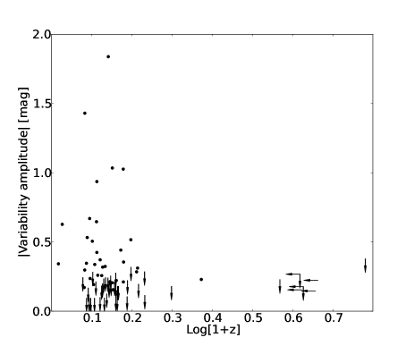
Figure 6: Correlation between redshift and variability amplitude. Uncertain redshifts as denoted from the SDSS pipeline flags are marked with a horizontal arrow.

Only 6 of the 107 ($\sim 5.6\%$) varying sources have neither a radio nor X-ray counterpart. Three out of those six have a reliable redshift so that only three objects are only variable and do not have any other of the properties discussed in this paper. That only 38 of the varying objects have a radio and X-ray counterpart reflects the shallowness of the X-ray data used.

4.2 Host galaxies

We were able to resolve the host galaxy in 66 targets; i.e., in 36% of the sample. The results for resolved targets are summarized in Table 4.2. Column 1 gives the target name, Col. 2 the telescope used, Col. 3 the redshift, listed only when the redshift determination is secure, Col. 4 the SDSS r’-band magnitude of the core, Col. 5 the SDSS r’-band magnitude of the host galaxy, Col. 6 the effective radius in arcsec, Col. 7 the ellipticity of the host galaxy, Col. 8 the position angle of the host galaxy, Col. 9 host galaxy type (U = undefined, B = bulge), Col. 10 the fraction of the core flux of the total flux, Col. 11 SDSS r’-band absolute magnitude, and Col. 12 the effective radius in kpc. In Appendix A, we show the surface brightness profiles of the resolved host galaxies, as well as the fits to them. In addition, one example of an unresolved and marginally resolved host galaxy based on the observations on each of the three telescopes used is displayed as well.

Table 3: Host galaxy results for the bulge model.

SDSS	Tel.	z	$m_{c}$	$m_{g}$	$r_{e}$	$\epsilon_{g}$	$\theta_{g}$	Host	Core	$M_{r^{\prime}}$	$r_{e}$
			(mag)	(mag)	(arcsec)		(deg)	type	frac	(mag)	(kpc)
000121.47-001140.3	NTT	0.4620	19.88 $\pm$ 0.15	19.78 $\pm$ 0.10	2.1 $\pm$ 0.6	0.39	-40	U	0.60 $\pm$ 0.07	-22.92	12.2
002200.95+000658.0	NTT	0.3057	-	18.53 $\pm$ 0.07	1.5 $\pm$ 0.2	0.10	61	B	(0.16 $\pm$ 0.07)	-22.74	6.7
002839.77+003542.2	NTT	-	19.76 $\pm$ 0.16	20.42 $\pm$ 0.26	2.4 $\pm$ 3.9	0.00	0	U	0.85 $\pm$ 0.10	-	-
010326.01+152624.8	NTT	0.2461	19.59 $\pm$ 0.22	17.04 $\pm$ 0.08	4.5 $\pm$ 0.5	0.30	-19	B	0.25 $\pm$ 0.04	-23.81	17.3
011012.66-004746.9	NTT	0.5477	20.16 $\pm$ 0.11	19.23 $\pm$ 0.18	8.2 $\pm$ 3.3	0.37	-45	U	0.69 $\pm$ 0.05	-24.15	52.4
012155.87-102037.2	NTT	0.4695	-	19.26 $\pm$ 0.09	0.7 $\pm$ 0.1	0.00	0	U	(0.20 $\pm$ 0.08)	-23.52	4.0
012750.83-001346.6	NTT	0.4376	20.36 $\pm$ 0.30	19.37 $\pm$ 0.10	1.6 $\pm$ 0.3	0.00	0	U	0.39 $\pm$ 0.09	-23.13	9.1
020106.18+003400.2	NTT	0.2985	19.27 $\pm$ 0.36	18.39 $\pm$ 0.09	2.0 $\pm$ 0.4	0.00	0	U	0.49 $\pm$ 0.09	-22.81	8.8
023813.68-092431.4	NTT	0.4188	-	19.27 $\pm$ 0.06	1.2 $\pm$ 0.1	0.18	-22	B	(0.07 $\pm$ 0.06)	-23.05	6.5
024302.93+004627.3	NTT	0.4089	20.55 $\pm$ 0.39	19.35 $\pm$ 0.09	1.2 $\pm$ 0.3	0.38	-32	U	0.33 $\pm$ 0.09	-22.89	6.3
024752.13+004106.3	NTT	0.3929	20.59 $\pm$ 0.23	19.72 $\pm$ 0.08	1.6 $\pm$ 0.3	0.47	7	B	0.44 $\pm$ 0.07	-22.41	8.7
025612.47-001057.8	NTT	0.6302	20.53 $\pm$ 0.16	19.98 $\pm$ 0.10	3.1 $\pm$ 0.9	0.25	-33	U	0.62 $\pm$ 0.07	-24.11	21.5
030433.96-005404.7	NTT	0.5112	18.69 $\pm$ 0.25	19.43 $\pm$ 0.23	1.8 $\pm$ 1.9	0.00	0	U	0.80 $\pm$ 0.14	-23.80	11.0
032356.64-010829.6	NTT	0.3923	20.67 $\pm$ 0.17	19.65 $\pm$ 0.09	2.7 $\pm$ 0.6	0.38	76	U	0.50 $\pm$ 0.07	-22.62	14.3
083918.75+361856.1	NOT	0.3343	20.14 $\pm$ 0.26	19.15 $\pm$ 0.11	1.5 $\pm$ 0.5	0.00	0	U	0.42 $\pm$ 0.09	-22.44	7.1
084225.52+025252.7	NTT	0.4251	19.94 $\pm$ 0.11	19.04 $\pm$ 0.07	2.4 $\pm$ 0.4	0.13	59	B	0.45 $\pm$ 0.04	-23.33	13.1
085638.50+014000.7	NTT	0.4479	19.83 $\pm$ 0.13	20.07 $\pm$ 0.11	1.2 $\pm$ 0.5	0.00	0	U	0.66 $\pm$ 0.07	-22.53	6.6
085749.80+013530.3	NTT	0.2812	18.79 $\pm$ 0.14	17.61 $\pm$ 0.07	1.8 $\pm$ 0.2	0.32	77	B	0.39 $\pm$ 0.05	-23.46	7.5
094432.33+573536.2	CA	-	19.69 $\pm$ 0.17	20.40 $\pm$ 0.26	1.5 $\pm$ 3.3	0.00	0	U	0.73 $\pm$ 0.10	-	-
094542.24+575747.7	NOT	0.2289	16.92 $\pm$ 0.21	16.89 $\pm$ 0.14	4.3 $\pm$ 1.9	0.00	0	U	0.72 $\pm$ 0.11	-23.51	15.7
094620.21+010452.1	NTT	0.5775	19.81 $\pm$ 0.24	20.35 $\pm$ 0.22	1.6 $\pm$ 2.6	0.00	0	U	0.74 $\pm$ 0.13	-23.60	10.7
095127.82+010210.2	NTT	-	19.97 $\pm$ 0.36	19.86 $\pm$ 0.17	0.9 $\pm$ 0.3	0.31	-19	U	0.55 $\pm$ 0.12	-	-
102013.78+625010.1	CA	0.2495	19.28 $\pm$ 0.19	17.67 $\pm$ 0.09	3.0 $\pm$ 0.4	0.00	0	B	0.35 $\pm$ 0.05	-22.97	11.6
102523.04+040229.0	NTT	0.2078	19.29 $\pm$ 0.11	17.87 $\pm$ 0.09	3.0 $\pm$ 0.5	0.12	-30	B	0.44 $\pm$ 0.04	-22.33	10.4
103220.29+030949.2	NTT	0.3233	18.86 $\pm$ 0.16	19.89 $\pm$ 0.22	1.2 $\pm$ 1.3	0.00	0	U	0.81 $\pm$ 0.09	-21.58	5.8
103940.70+053609.3	NTT	0.5103	20.31 $\pm$ 0.25	20.02 $\pm$ 0.10	0.9 $\pm$ 0.5	0.00	0	U	0.52 $\pm$ 0.10	-23.04	5.6
105151.84+010310.7	NTT	0.2654	18.51 $\pm$ 0.11	19.40 $\pm$ 0.13	2.1 $\pm$ 1.0	0.28	67	U	0.84 $\pm$ 0.07	-21.52	8.4
105606.62+025213.5	NTT	0.2360	19.67 $\pm$ 0.21	18.11 $\pm$ 0.08	1.8 $\pm$ 0.4	0.10	73	B	0.36 $\pm$ 0.06	-22.46	6.7
105752.79-005908.3	NTT	-	20.11 $\pm$ 0.24	20.87 $\pm$ 0.28	0.8 $\pm$ 1.8	0.00	0	U	0.72 $\pm$ 0.13	-	-
110356.15+002236.4	NTT	0.2747	19.47 $\pm$ 0.12	17.87 $\pm$ 0.08	3.4 $\pm$ 0.4	0.22	84	B	0.40 $\pm$ 0.03	-23.12	14.2
110704.78+501037.9	CA	0.7061	20.27 $\pm$ 0.26	20.12 $\pm$ 0.22	0.7 $\pm$ 0.3	0.00	0	U	0.48 $\pm$ 0.11	-24.38	4.9
111717.55+000633.6	NTT	0.4511	19.19 $\pm$ 0.14	19.56 $\pm$ 0.12	1.0 $\pm$ 0.3	0.22	36	U	0.67 $\pm$ 0.08	-23.07	5.8
115404.54-001009.9	NTT	0.2535	18.82 $\pm$ 0.15	18.31 $\pm$ 0.09	1.6 $\pm$ 0.4	0.00	0	U	0.55 $\pm$ 0.07	-22.39	6.3
120303.50+603119.1	CA	0.0653	16.50 $\pm$ 0.10	14.82 $\pm$ 0.09	7.4 $\pm$ 0.8	0.02	77	B	0.46 $\pm$ 0.03	-22.56	9.3
121758.72-002946.2	NTT	0.4188	19.39 $\pm$ 0.15	19.32 $\pm$ 0.22	1.6 $\pm$ 1.8	0.00	0	U	0.59 $\pm$ 0.08	-22.99	9.0
121944.98+044622.4	NTT	0.4891	18.54 $\pm$ 0.12	19.83 $\pm$ 0.22	1.0 $\pm$ 1.2	0.00	0	U	0.84 $\pm$ 0.08	-23.05	6.2
122300.31+515313.9	CA	0.3650	19.76 $\pm$ 0.12	19.46 $\pm$ 0.10	2.0 $\pm$ 0.5	0.00	0	U	0.57 $\pm$ 0.05	-22.37	10.2
122809.13-022136.1	NTT	0.3227	20.73 $\pm$ 0.29	19.36 $\pm$ 0.07	0.8 $\pm$ 0.1	0.18	-58	B	0.27 $\pm$ 0.06	-22.09	3.6
124225.39+642919.1	CA	0.0424	-	15.51 $\pm$ 0.08	4.7 $\pm$ 0.4	0.24	66	B	(0.05 $\pm$ 0.05)	-20.91	3.9
124425.30+044459.7	NTT	0.3999	-	19.46 $\pm$ 0.07	1.1 $\pm$ 0.1	0.40	-34	U	(0.16 $\pm$ 0.07)	-22.69	5.9
124834.30+512807.8	CA	0.3508	18.19 $\pm$ 0.20	18.86 $\pm$ 0.26	1.0 $\pm$ 0.6	0.00	0	U	0.71 $\pm$ 0.11	-22.81	4.7
125820.79+612045.6	CA	0.2235	-	18.09 $\pm$ 0.07	0.6 $\pm$ 0.1	0.00	0	B	(0.00 $\pm$ 0.00)	-22.27	2.1
131330.15+020105.9	NTT	0.3558	18.85 $\pm$ 0.07	18.50 $\pm$ 0.20	5.3 $\pm$ 2.9	0.21	69	U	0.73 $\pm$ 0.04	-23.25	26.2
132301.01+043951.4	NTT	0.2244	18.41 $\pm$ 0.11	17.65 $\pm$ 0.09	3.0 $\pm$ 0.8	0.12	9	U	0.58 $\pm$ 0.05	-22.75	10.8
132759.76+645811.3	CA	0.4468	-	18.71 $\pm$ 0.08	2.1 $\pm$ 0.3	0.23	-69	B	(0.04 $\pm$ 0.06)	-23.84	12.2
133105.71-002221.2	NTT	0.2426	20.80 $\pm$ 0.33	18.37 $\pm$ 0.05	1.1 $\pm$ 0.1	0.11	-54	B	0.14 $\pm$ 0.04	-22.23	4.1
134037.59-014847.6	NTT	0.5130	20.11 $\pm$ 0.16	20.25 $\pm$ 0.09	1.5 $\pm$ 0.8	0.00	0	U	0.69 $\pm$ 0.09	-22.87	9.2
141003.92+051557.7	NTT	0.5440	20.25 $\pm$ 0.09	19.69 $\pm$ 0.08	2.1 $\pm$ 0.4	0.24	-24	B	0.55 $\pm$ 0.04	-23.65	13.6
141030.84+610012.8	CA	0.3833	20.08 $\pm$ 0.20	19.18 $\pm$ 0.09	1.3 $\pm$ 0.2	0.00	0	U	0.36 $\pm$ 0.06	-22.80	6.7
145111.69+580003.0	CA	0.4053	20.13 $\pm$ 0.31	18.84 $\pm$ 0.10	2.4 $\pm$ 0.5	0.34	21	U	0.33 $\pm$ 0.08	-23.32	13.2
150006.49+012956.0	NTT	0.7083	20.18 $\pm$ 0.19	21.38 $\pm$ 0.27	1.0 $\pm$ 2.5	0.00	0	U	0.83 $\pm$ 0.11	-23.21	7.1
161541.22+471111.8	CA	0.1986	18.09 $\pm$ 0.13	17.32 $\pm$ 0.09	2.8 $\pm$ 0.4	0.00	0	U	0.53 $\pm$ 0.05	-22.70	9.0
162115.21-003140.4	NTT	-	19.73 $\pm$ 0.10	20.34 $\pm$ 0.13	0.6 $\pm$ 0.1	0.00	0	U	0.68 $\pm$ 0.06	-	-
165109.18+421253.5	CA	0.2686	-	18.85 $\pm$ 0.12	1.0 $\pm$ 0.2	0.00	0	U	(0.15 $\pm$ 0.11)	-22.04	4.1
165808.33+615001.9	NOT	0.3742	18.64 $\pm$ 0.23	18.42 $\pm$ 0.16	2.0 $\pm$ 1.0	0.00	0	U	0.64 $\pm$ 0.10	-23.56	10.3
205523.36-050619.3	NTT	0.3426	19.65 $\pm$ 0.16	18.52 $\pm$ 0.08	2.2 $\pm$ 0.4	0.22	-24	U	0.38 $\pm$ 0.05	-23.25	10.5
205938.57-003756.0	NTT	0.3354	20.17 $\pm$ 0.22	18.72 $\pm$ 0.08	2.2 $\pm$ 0.4	0.21	31	U	0.37 $\pm$ 0.06	-22.97	10.5
211611.89-062830.4	NTT	0.2916	19.51 $\pm$ 0.44	18.64 $\pm$ 0.13	0.8 $\pm$ 0.2	0.00	0	U	0.37 $\pm$ 0.11	-22.78	3.7
213950.32+104749.6	NTT	0.2960	21.55 $\pm$ 0.49	17.68 $\pm$ 0.09	8.4 $\pm$ 1.2	0.28	89	B	0.11 $\pm$ 0.04	-23.59	37.2
215051.73+111916.5	NTT	-	19.47 $\pm$ 0.19	20.04 $\pm$ 0.18	1.2 $\pm$ 0.8	0.00	0	U	0.70 $\pm$ 0.11	-	-
215305.36-004230.7	NTT	0.3416	18.98 $\pm$ 0.34	18.85 $\pm$ 0.24	0.5 $\pm$ 0.3	0.00	0	U	0.50 $\pm$ 0.14	-23.02	2.3
221108.34-000302.5	NTT	0.3619	18.97 $\pm$ 0.29	19.12 $\pm$ 0.18	0.6 $\pm$ 0.2	0.33	57	U	0.58 $\pm$ 0.11	-22.78	3.3
221109.88-002327.5	NTT	0.4476	20.17 $\pm$ 0.23	19.08 $\pm$ 0.07	2.0 $\pm$ 0.4	0.20	54	U	0.43 $\pm$ 0.07	-23.64	11.6
221456.37+002000.1	NTT	-	19.69 $\pm$ 0.16	20.44 $\pm$ 0.21	1.7 $\pm$ 1.7	0.00	0	U	0.77 $\pm$ 0.10	-	-
224819.44-003641.6	NTT	0.2123	19.87 $\pm$ 0.24	17.15 $\pm$ 0.07	4.3 $\pm$ 0.6	0.11	37	B	0.19 $\pm$ 0.04	-23.28	14.8
235604.03-002353.8	NTT	0.2830	19.72 $\pm$ 0.23	19.05 $\pm$ 0.09	1.2 $\pm$ 0.3	0.22	50	U	0.46 $\pm$ 0.08	-22.01	5.2

The absolute magnitudes $M_{r^{\prime}}$ in Table 4.2 were computed from

$$M_{r^{\prime}}=m_{g}-DM-K_{r^{\prime}}-A_{r^{\prime}}+E(z)\ ,$$ (6)

where $DM$ is the distance modulus, $K_{r^{\prime}}$ is the K correction (Fukugita et al. 1995), $A_{r^{\prime}}$ is the galactic extinction (Schlegel et al. 1998), and $E(z)=0.93\cdot z$ is the evolution correction. The latter was computed using the PEGASE code (Fioc & Rocca-Volmerange 1997) by assuming initial ISM metallicity $Z_{0}=0.004$, single starburst 11 Gyr ago (z = 2.6), and passive evolution thereafter.

None of the targets were unambiguously associated with a disk type galaxy. In seven cases out of 66 a disk host galaxy formally gave a better fit, but the simulations showed that in none of these cases the host galaxy type was secure. In all 19 cases where our simulations showed the host galaxy type to be well determined the bulge model was preferred. This result is in line with previous BL Lac host galaxy imaging surveys (e.g., Urry et al. 2000; Nilsson et al. 2003), which show that BL Lacs are almost exclusively found in ellipticals. Given this result we use the bulge fit results for all targets from this point on.

As Table 4.2 indicates, in eight cases we were not able to detect an optical core. In seven cases out of these eight the fit returned a value for the core magnitude $m_{c}$, but subsequent error simulations indicated that the error of $m_{c}$ was $>$ 0.5 mag. We mark these cores as undetected, although it is possible that weak cores below our detection limit are present in these targets or the objects were in a very low state. Column 10 on Table 4.2 gives the core fraction; i.e., the ratio between the core flux and total flux within the aperture used for polarimetry in Paper I. This was measured directly from the two-dimensional model images of the core and the host galaxy using aperture photometry. We list in parenthesis the core fraction also for the eight targets with formally undetected cores, computed from the core magnitude returned by the fit. The formal core fractions of the non-detected cores are very low, 0.04-0.20, as expected. The only case in which the fit converged toward $m_{c}\rightarrow\infty$, i.e. core fraction of 0.0, is SDSS125820.79+612045.6, which is the only target where we have no evidence of an optical core.

SDSS012155.87-102037.2: A disk fit formally gives a better fit, but both bulge and disk fits leave strong residuals, which are unlikely to be due to PSF verifiability and give an impression of a tight gravitational lens system or a merger of several galaxies. A weak core is indicated by the fits, but not significantly detected.

SDSS094432.33+573536.2: There are two compact objects within 3.0 arcsec from the core.

SDSS100050.22+574609.1: This is one of the targets with only marginal detection of the host galaxy. The nucleus is surrounded by a very elongated feature giving an impression of a nearly edge-on disk galaxy.

4.3 Optical spectra

All the obtained and reduced spectra can be found in the Appendix 8. In spite of our high S/N spectra for only one out of our 27 objects a unique redshift could be assigned. SDSS J105829.62+013358.8 shows a very broad emission feature at 5289Å, which was identified with MgII yielding a redshift of z=0.89$\pm$0.02. In the SDSS-pipeline (DR8 and earlier), the broad feature was identified as CIII (z=1.78$\pm$0.003), but in the following data releases, the feature was also attributed to MgII emission at z = 0.8933$\pm$0.0004. Out of the remaining 26 objects, 17 have at least one absorption/emission line in their spectra, while the spectra of the remaining 9 objects appear featureless. No unique redshift could be assigned for the 17 objects with a single emission/absorption line, .

Table 4 with our analysis of the spectroscopic data as well as the median-combined spectra for all objects, can be found the Appendix. In Table 4 the target name, the r-band magnitude from SDSS, the S/N per resolution element at 6500Å  in the spectra and the central wavelength for the emission/absorption lines detected is given . We also indicate their equivalent widths.

4.4 Broadband SEDs

The main scope of polynomial fits to the SEDs was to derive the synchrotron peak frequencies for the objects in our sample. As shown in Fig. 7, most of the objects have peak frequencies between $13.5\leq\mathrm{log}_{10}\left(\nu_{\mathrm{peak}}\right)\leq 16$ with a faint tail towards higher frequencies. This is a similar range to the one found by Nieppola et al. (2008), although the peak frequencies they derived are shifted toward lower frequencies. This is due to their sample selection of radio-bright blazars. The distribution is not homogeneous but rather peaked at $\mathrm{log}_{10}\sim 14.5$. Thus the sample seems to contain a substantial fraction of IBL.

The derived synchrotron peak frequencies are affected by variability, temporal evolution of the peak frequency, shallowness of the data, and a significant host galaxy component in some cases. We made Monte Carlo simulations where the photometric data points were varied within their errors, which showed that photometric errors alone can cause shifts in the peak frequency up to 0.2 in the logarithmic scale. Variability and peak shifts are difficult to account, for and we also did not subtract the host galaxy light since we expect that the influence to the general distribution is very low, although in some individual cases there might be larger shifts because of the host galaxy light.

For three of our objects, the SED fits yielded extremely high peak frequencies. The SED of SDSS J094432.34+573536.15 shows almost a linear slope while SDSS J104523.87+015722.09 seems to be dominated by black body radiation. The latter source was identified by Kleinman et al. (2004) as a DC white dwarf but not confirmed by Eisenstein et al. (2006). This source is apparently a radio source (Collinge et al. 2005). FIRST lists a 2.7mJy radio source about 1.3” south of the SDSS position, where a faint optical counterpart is present on our NTT image. Both objects may have entered the 3″SDSS fiber, and the resulting spectrum be a superposition from both components. SDSS J140450.91+040202.16 would finally yield a synchrotron peak between $15\leq\mathrm{log10}\left(\nu_{\mathrm{peak}}\right)\leq 16$ when X-ray data would have been taken into account.

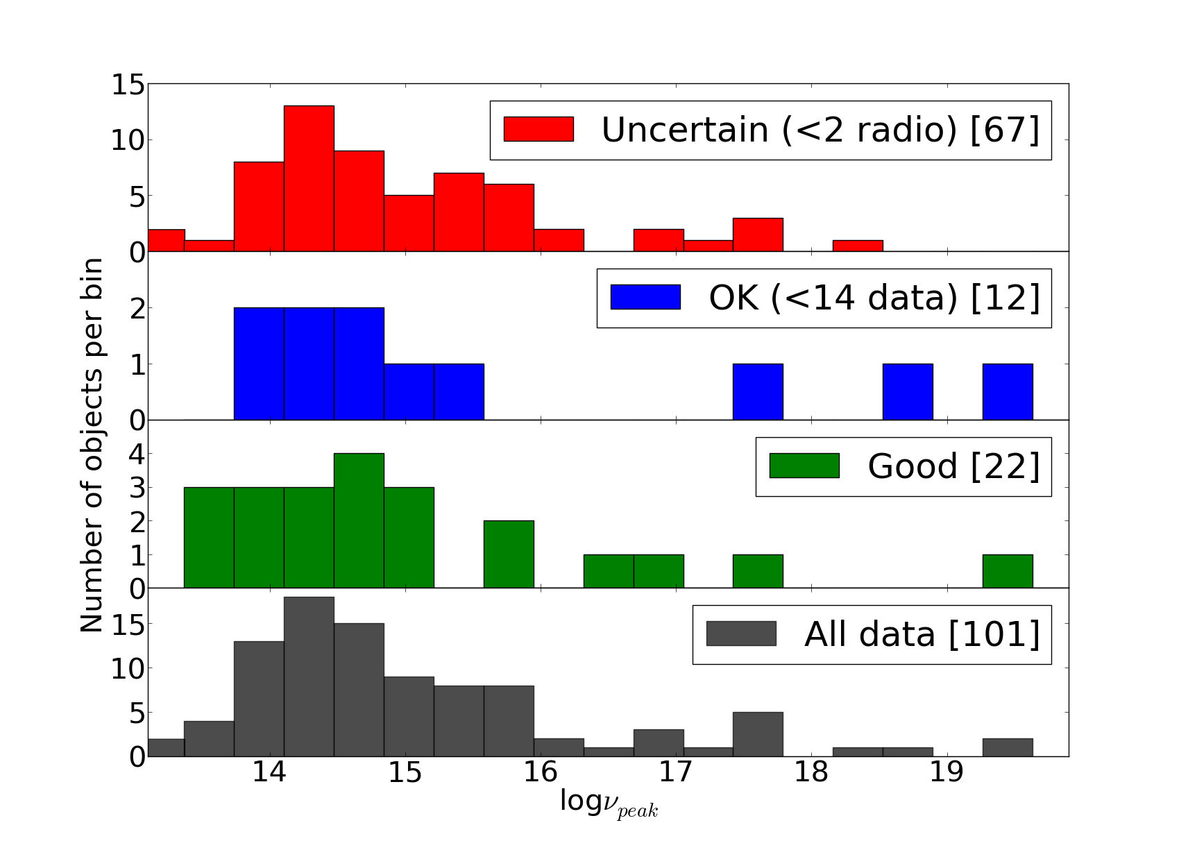
Figure 7: Distribution of frequency peaks for the different quality classes. For better clarity the 6 (5 uncertain, 1 OK) objects above $\mathrm{log10}\left(\nu_{\mathrm{peak}}\right)>20$ are not shown.

In Table A in the Appendix, we summarize the global properties of our targets derived in Paper I and in this work. This includes the redshifts from SDSS, the spectral indices $\alpha_{ox}$ and $\alpha_{ro}$, the polarization properties, the variability limit and variabiliy amplitudes, the core fraction derived from the host galaxy and the peak-frequencies from the SED fits.

5 Summary

We presented a detailed analysis of the properties of 182 probable BL Lac candidates from the SDSS extracted by Collinge et al. (2005). Particular emphasis was given to their variability characteristics and their broad-band radio-UV SEDs. We also examined our data for the presence of a host galaxy of the targets. In addition, we presented new optical spectra of 27 targets with improved S/N with respect to the SDSS spectra. Our main results can be summarized as follows:

• About 60% (107/182) of the objects show variability on long timescales between SDSS DR2 and our observations in 2008-09. The 3$\sigma$ confidence interval for the number of variable targets, when taking only observational errors into account, is (99 119).

• Using two-dimensional model fits, we were able to resolve the host galaxy in 66 targets, 7 of them without a secure SDSS redshift. None of the host galaxies is unambiguously associated with a disk galaxy. In the 19 cases where the host galaxy classification is unique, a deVaucouleurs model is preferred. The luminosity distribution is consistent with earlier results of BL Lac host galaxies if a bias in the sample is taken into account.

• We analyzed 104 broad-band radio-UV SEDs and determined the synchrotron peak frequency. The objects have peak frequencies between $13.5\leq\mathrm{log}_{10}\left(\nu_{\mathrm{peak}}\right)\leq 16$ with a faint tail toward higher frequencies. The distribution is not homogeneous but instead peaked at $\mathrm{log}_{10}\sim 14.5$. Thus the sample seems to contain a substantial fraction of IBL.

• Our new optical spectra did not reveal any new redshift for any of our objects. For SDSS J105829.62+013358.8, we could confirm the SDSS redshift of z = 0.89$\pm$0.02.

• There is potentially a population of high-redshift BL Lacs as indicated in Fig. 6 with low variability amplitudes. This could alternatively be a different class of objects (high-redshift weak-lined QSOs) or an artifact due to wrong redshift assignments.

Overall, our results, including the analysis of the polarimetric properties imply that the Collinge et al. (2005) sample, is only marginally contaminated by stellar sources and is likely to contain a high fraction of bona fide BL Lacs. It potentially contains a high fraction of IBL. The detailed discussion of these properties, a comparison to BL Lac samples determined by other selection criteria and a potential revision of the defining criteria of a BL Lac will be presented in a forthcoming paper (Nilsson et al., in prep).

Appendix A Appendix

Table 4: Results of the analysis of the optical spectra. Negative EW indicate absorption lines.

Nr	Object name	$r_{SDSS}$	S/N per RE	Lines
	[SDSS]	[mag]	at $\lambda$ 6500$\mathring{A}$	CWL / EW [$\mathring{A}$]
I	J003514.72+151504.1	16.59	174	5721 / -0.42
II	J011452.77+132537.5	17.03	186	7545 / 0.34
III	J022048.46$-$084250.4	18.27	62	-
IV	J032343.62$-$011146.1	16.81	174	7188 / -3.02, 8168 / -2.44
V	J074054.60+322601.0	18.67	62	7536 / 4.10
VI	J085920.56+004712.1	18.76	37	5049 / -0.33
VII	J091848.57+021321.8	18.55	37	-
VIII	J100612.23+644011.6	18.87	62	7127 / 3.52
IX	J101858.55+591127.8	17.75	87	-
X	J105829.62+013358.8	17.86	112	5289 / 9.27 , 8175 / -1.08 (z=0.89$\pm$0.02)
XI	J110735.92+022224.5	18.59	37	-
XII	J113245.61+003427.7	17.44	99	-
XIII	J113523.70+660941.0	18.94	37	8082 / -3.52, 8146 / -3.33
XIV	J114312.11+612210.8	17.93	99	5001 / 0.42
XV	J114926.13+624332.5	18.93	25	8288 / 5.24
XVI	J121300.80+512935.6	18.45	62	-
XVII	J121500.80+500215.6	17.41	74	-
XVIII	J121834.93$-$011954.3	17.55	136	6970 / 2.8 , 7196 / -0.53
XIX	J123341.33$-$014423.7	18.31	50	5995 / 1.2
XX	J131106.48+003510.0	17.86	99	5419 / 0.40
XXI	J135738.70+012813.6	17.82	74	-
XXII	J140450.91+040202.2	16.31	186	7188 / -1.89, 8160 / -1.98
XXIII	J141004.65+020306.9	18.15	87	8384 / 3.40
XXIV	J141826.33$-$023334.1	16.64	174	7193 / -2.88
XXV	J141927.50+044513.8	18.18	50	6336 / -6.13
XXVI	J143657.71+563924.8	18.42	50	7518 / 3.6
XXVII	J170124.64+395437.1	16.88	223	-

2

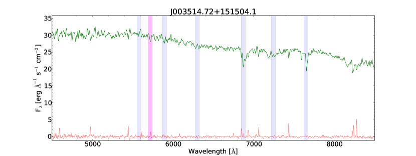
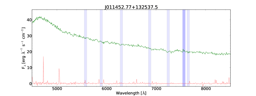
Figure 8: Flux-calibrated spectra. The green lines are the binned (factor of 2) spectra with the red lines representing the typical error (obtained by IRAF - routines) of the respective data point. Features stemming from an imperfect sky-subtraction are marked in light gray, significant (5$\sigma$ in all 3 spectra or 10$\sigma$ in 2/3 spectra) absorption/emission features originating in the object are marked light magenta/blue.

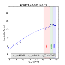
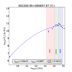
Figure 9: SED fits, and peak frequencies of all objects with more than 12 data points in the SED. All objects with fewer than 2 radio measurements (uncertain) are labeled with a “[?]” in the figure caption. The three objects where the fit did not yield any reasonable results are emphasized with a “*” and objects with a significant influence of the host galaxy (core fraction $<$ 0.5) on the SED are highlighted with a “$\dagger$” in the title.

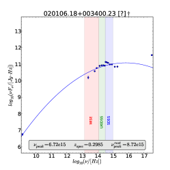
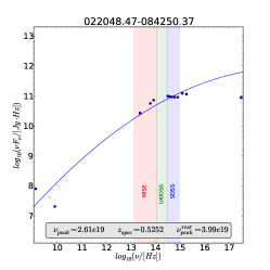
Figure 1: –Continued.

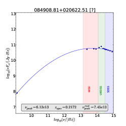
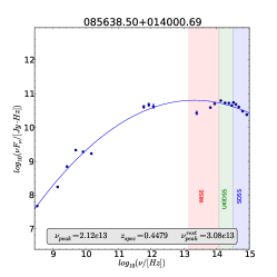
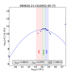
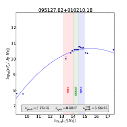
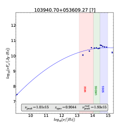
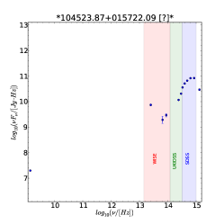
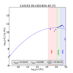
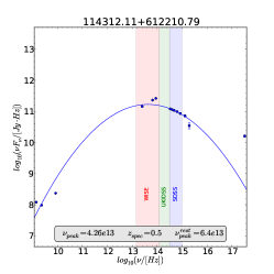
Figure 1: –Continued.

Figure 1: –Continued.

Figure 1: –Continued.

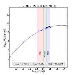
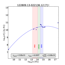
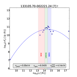
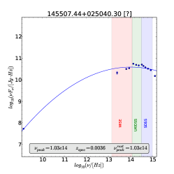
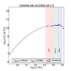
Figure 1: –Continued.

Figure 1: –Continued.

Figure 1: –Continued.

Figure 1: –Continued.

Figure 2: Surface brightness (SB) profiles of the targets with detected host galaxies. Horizontal axis gives the distance from the center in arcsec and the vertical axis the surface brightness in mag/sq. arcsec. In addition to the observed SB, we show the SB of the total core + host galaxy model (solid line), the core model (dashed line) and the host galaxy model (dotted line).

Figure 1: –Continued.

Figure 1: –Continued.

Figure 1: –Continued.

Figure 2: Examples of unresolved (top row) and marginally resolved (bottom row) targets. From left to right: NTT, CA, and NOT data.

Table 5: Main properties objects discussed in Heidt & Nilsson (2011) and the present work. Cols. 2 and 3 the spectroscopic redshift from SDSS and flags, Cols. 4 and 5 spectral indices $\alpha_{ox}$ and $\alpha_{ro}$. All these properties are from Collinge et al. (2005). Cols. 6 and 7 give the polarization and its error, Col. 8 the variability limit, Col. 9 the variability amplitude, Cols. 10 and 11 the core (AGN) fraction over the total flux fraction as derived from the host galaxy fits and their error, Col. 12 the peak frequency determined from SED fits, and Col. 13 a flag with respect to the SED fits. The flags indicate whether the peak estimate is uncertain due to the shallowness of the radio data (“radio” if only one or no radio point available) or due to the presence of a strong host galaxy if the host galaxy fraction of the total flux exceeds 0.5 (flag is“galaxy”).

[x]ccccccccccccc Target name & z${}_{\text{SDSS}}$ z${}_{\text{SDSS}}$ aox aro pol ePol VL Var core error log$\left(\nu_{\text{Peak}}\right)$ SED Flag frac frac Flag $[$SDSS J$]$ $[$%$]$ $[$%$]$ $[$mag$]$ $[$mag$]$ $[$log$\left(\text{Hz}\right)]$

Table A $-$ Continued.

Target name z${}_{\text{SDSS}}$ z${}_{\text{SDSS}}$ aox aro pol ePol VL Var core error log$\left(\nu_{\text{Peak}}\right)$ SED Flag frac frac Flag $[$SDSS J$]$ $[$%$]$ $[$%$]$ $[$mag$]$ $[$mag$]$ $[$log$\left(\text{Hz}\right)]$ 000121.47$-$001140.3 0.4620 - $>$0.98 0.63 4.34 0.75 0.06 -0.103 0.60 0.07 16.59 - 002142.26$-$090044.4 0.6481 - $>$1.07 0.51 12.80 0.83 0.065 0.104 1 - - - 002200.95+000658.0 0.3057 - 0.94 0.28 $<$2.56 - 0.064 0.259 $<$0.16 0.07 15.21 radio 002839.77+003542.2 0.6866 u $>$1.00 0.49 4.45 0.69 0.072 0.519 0.85 0.10 17.43 - 003514.72+151504.1 - - 1.16 0.25 6.90 0.96 0.087 1.057 1 - 17.29 radio 004054.65$-$091526.8 5.0300 - $>$1.01 $<$0.05 $<$3.99 - 0.126 0.105 1 - - - 005041.31$-$092905.1 - - 1.28 0.55 19.01 0.35 0.05 -0.641 1 - 15.08 radio 010058.19$-$005547.8 $>$0.6679 u $>$1.04 0.49 12.82 0.66 0.057 -0.262 1 - 13.53 - 010326.01+152624.8 0.2461 - $>$1.22 0.60 1.62 0.68 0.068 0.669 0.25 0.04 16.81 radio 011012.66$-$004746.9 0.5477 - $>$0.94 0.54 5.52 0.90 0.074 0.122 0.69 0.05 14.34 - 011452.77+132537.5 - - $>$1.34 0.41 9.10 0.61 0.057 0.801 1 - 14.8 radio 012155.87$-$102037.2 0.4695 - $>$1.02 $<$0.23 $<$0.90 - 0.06 0.005 $<$0.20 0.08 - - 012227.38+151023.1 - - $>$0.89 0.55 10.41 1.05 0.07 0.557 1 - 13.63 - 012716.31$-$082128.9 0.3620 u $>$1.04 0.66 6.32 0.87 0.067 0.203 1 - - - 012750.83$-$001346.6 0.4376 - $>$0.98 0.40 4.13 0.78 0.07 -0.032 0.39 0.09 14.33 radio 013408.95+003102.5 - - $>$0.93 $<$0.29 $<$2.03 - 0.067 0.035 1 - - - 014125.83$-$092843.7 $>$0.5000 u 1.45 0.60 4.88 0.56 0.067 0.88 1 - 13.93 - 020106.18+003400.2 0.2985 - 0.89 0.38 1.37 0.67 0.061 0.424 0.49 0.09 15.83 radio 020137.66+002535.1 - - $>$0.99 $<$0.26 $<$2.18 - 0.065 0.109 1 - - - 022048.46$-$084250.4 0.5252 u 1.09 0.49 6.09 0.45 0.054 -0.355 1 - 19.42 - 023813.68$-$092431.4 0.4188 - 1.09 0.34 2.51 0.70 0.067 0.205 $<$0.07 0.06 14.52 galaxy 024156.38+004351.6 0.9900 - $>$0.90 0.11 2.60 0.72 0.06 0.026 1 - - - 024157.37+000944.1 0.7896 u 0.83 0.32 4.03 1.63 0.114 0.303 1 - 14.14 radio 024302.93+004627.3 0.4089 - $>$0.96 0.53 $<$3.17 - 0.07 0.106 0.33 0.09 - - 024752.13+004106.3 0.3929 - $>$0.82 0.41 $<$2.40 - 0.066 -0.086 0.44 0.07 13.91 radio 025046.48$-$005449.0 - - $>$0.74 $<$0.28 $<$2.95 - 0.082 0.095 1 - - - 025612.47$-$001057.8 0.6302 - $>$-0.11 $<$0.28 $<$2.42 - 0.076 -0.284 0.62 0.07 14.11 radio 030235.78$-$075027.0 - - $>$0.71 0.45 8.42 0.71 0.064 -0.497 1 - - - 030240.30+003849.9 - - $>$0.73 0.33 $<$1.93 - 0.066 0.041 1 - 14.04 - 030433.96$-$005404.7 0.5112 - 1.03 0.44 1.83 0.60 0.059 -0.211 0.80 0.14 14.99 radio 031712.23$-$075850.4 2.6993 - $>$1.03 - $<$3.20 - 0.076 0.075 1 - - - 032343.62$-$011146.1 - - 1.35 0.32 5.22 0.98 0.067 0.789 1 - 15.4 radio 032356.64$-$010829.6 0.3923 - 0.89 0.41 $<$2.13 - 0.071 0.052 0.50 0.07 13.38 radio 040911.36$-$055529.4 - - $>$0.93 0.53 9.76 1.33 0.079 0.629 1 - - - 045128.96$-$002911.5 - - $>$0.75 0.80 $<$3.98 - 0.078 0.138 1 - - - 074054.60+322601.0 $>$0.9460 u $>$1.09 0.38 5.44 0.83 0.051 0.002 1 - - - 075144.94+392817.6 0.4338 u $>$0.80 0.44 3.99 1.78 0.099 -0.921 1 - - - 075602.72+414039.8 0.5788 - $>$0.94 0.36 $<$6.09 - 0.106 -0.216 1 - - - 081840.06+315348.2 - - $>$1.01 0.57 14.48 1.17 0.077 -0.381 1 - - - 083413.90+511214.7 - - $>$1.05 0.26 $<$5.61 - 0.092 -0.156 1 - - - 083918.75+361856.1 0.3343 - $>$0.95 0.40 $<$2.92 - 0.061 0.066 0.42 0.09 18.42 galaxy 084225.52+025252.7 0.4251 - 1.15 0.45 $<$1.57 - 0.033 0.155 0.45 0.04 17.53 radio 084908.81+020622.5 - - $>$1.06 0.55 10.94 0.71 0.033 0.206 1 - 13.79 radio 085638.50+014000.7 0.4479 - $>$1.03 0.38 $<$3.78 - 0.034 0.088 0.66 0.07 13.33 - 085749.80+013530.3 0.2812 - 1.20 0.51 4.50 0.68 0.031 0.051 0.39 0.05 14.97 radio 085920.56+004712.1 - - 0.84 0.52 4.20 0.91 0.057 0.518 1 - 14.98 radio 090133.43+031412.5 0.4591 - $>$1.04 $<$0.21 $<$2.08 - 0.033 0.03 1 - 20.39 radio 090939.84+020005.3 - - $>$1.00 0.73 18.99 0.49 0.035 -1.101 1 - 13.33 radio 091848.57+021321.8 - - $>$1.13 0.32 4.29 1.16 0.058 0.896 1 - 14.49 radio 092542.87+595816.3 - - 1.03 0.40 8.65 1.10 0.078 0.171 1 - - - 092638.88+541126.7 0.8500 u $>$1.09 0.51 7.02 0.93 0.077 -0.55 1 - - - 092912.25+030029.9 - - $>$1.00 0.24 9.41 0.69 0.04 -0.345 1 - 12.9 radio 094245.30+541620.4 - - $>$0.99 0.45 7.51 2.17 0.104 0.024 1 - 15.39 - 094257.81$-$004705.2 1.3600 - $>$1.02 0.23 $<$1.62 - 0.033 -0.229 1 - 13.84 radio 094432.33+573536.2 - - 0.85 0.32 3.41 1.29 0.088 -0.32 0.73 0.10 - - 094432.33+573536.2 - - 0.85 0.32 8.06 0.61 0.088 -0.32 0.73 0.10 - - 094441.48+555753.1 - - $>$1.05 0.53 $<$4.48 - 0.088 -0.198 1 - - - 094542.24+575747.7 0.2289 - 1.53 0.48 4.90 0.22 0.04 -0.532 0.72 0.11 14.87 - 094620.21+010452.1 0.5775 - 0.81 0.42 4.86 0.56 0.038 -0.516 0.74 0.13 14.03 radio 095127.82+010210.2 - - 1.13 0.46 4.36 0.69 0.057 -0.029 0.55 0.12 15.58 - 095649.53+015601.8 - - 0.80 0.43 7.10 1.60 0.043 0.403 1 - 16.01 - 100050.22+574609.1 0.6392 - $>$1.16 0.58 5.14 1.22 0.088 0.311 1 - 13.63 - 100326.63+020455.7 - - $>$1.00 0.38 10.21 1.07 0.035 0.363 1 - 14.62 - 100612.23+644011.6 - - 1.07 0.53 8.81 1.01 0.074 -0.49 1 - - - 100959.63+014533.8 $>$1.0900 u $>$0.99 0.55 14.98 1.35 0.038 1.034 1 - 13.36 - 101115.64+010642.7 0.8615 u $>$0.95 0.70 $<$1.64 - 0.058 0.203 1 - 14.31 radio 101858.55+591127.8 - - $>$1.40 0.50 19.08 0.46 0.046 0.102 1 - 19.47 - 101950.87+632001.6 - - $>$1.28 0.56 7.80 0.65 0.072 -0.885 1 - 13.68 - 102013.78+625010.1 0.2495 - 1.22 0.49 $<$3.77 - 0.076 0.236 0.35 0.05 - - 102243.73$-$011302.5 - - 0.93 0.39 $<$2.56 - 0.031 -0.122 1 - 20.08 radio 102523.04+040229.0 0.2078 - 1.11 0.52 1.49 0.61 0.032 0.171 0.44 0.04 15.36 radio 102724.97+631753.1 $>$0.5816 - 1.14 0.41 11.51 1.06 0.077 -0.181 1 - - - 103208.36+040157.0 - - $>$0.99 0.65 11.84 0.49 0.057 -0.024 1 - - - 103220.29+030949.2 0.3233 - $>$1.18 0.45 4.92 0.71 0.032 0.371 0.81 0.09 13.8 radio 103239.07+662323.3 - - $>$1.13 0.60 3.26 1.09 0.074 -0.074 1 - - - 103940.70+053609.3 0.5103 - $>$0.73 0.38 $<$4.01 - 0.032 -1.026 0.52 0.10 15.01 radio 104523.86+015722.1 - - $>$0.96 0.30 $<$1.61 - 0.033 -0.186 1 - - - 104833.57+620305.0 - - $>$1.07 $<$0.27 $<$1.72 - 0.055 -0.296 1 - - - 105151.84+010310.7 0.2654 - $>$1.06 0.42 1.92 0.35 0.034 -0.74 0.84 0.07 14.21 radio 105151.84+010310.7 0.2654 - $>$1.06 0.42 4.86 0.33 0.034 -0.74 0.84 0.07 14.21 radio 105606.62+025213.5 0.2360 - 0.72 0.32 1.16 0.39 0.056 0.089 0.36 0.06 15.77 - 105752.79$-$005908.3 0.4678 u 0.94 0.29 $<$3.90 - 0.033 0.254 0.72 0.13 15.37 radio 105829.62+013358.8 0.8862 u 1.16 0.76 15.10 0.27 0.031 -1.712 1 - 12.77 radio 110356.15+002236.4 0.2747 - $>$1.12 0.52 4.38 0.36 0.056 0.192 0.40 0.03 14.89 galaxy 110704.78+501037.9 0.7061 - $>$1.14 0.49 4.27 1.66 0.095 0.035 0.48 0.11 - - 110735.92+022224.5 $>$1.0750 u $>$1.09 0.40 9.39 0.42 0.032 -0.233 1 - 14.59 radio 111717.55+000633.6 0.4511 - 0.87 0.44 1.46 0.52 0.036 0.803 0.67 0.08 15.46 radio 111717.55+000633.6 0.4511 - 0.87 0.44 1.87 0.52 0.036 0.803 0.67 0.08 15.46 radio 113115.50+023450.2 $>$0.4538 u $>$1.16 0.38 $<$2.79 - 0.033 0.811 1 - 14.22 - 113234.38+023740.3 - - $>$1.02 0.59 $<$1.83 - 0.034 0.078 1 - 17.99 radio 113245.61+003427.7 - - 1.48 0.61 6.35 0.68 0.056 0.092 1 - 13.54 radio 113523.70+660941.0 - - $>$1.18 0.56 13.52 2.16 0.051 0.731 1 - - - 113523.70+660941.0 - - $>$1.18 0.56 12.43 0.83 0.051 0.731 1 - - - 114153.35+021924.4 3.5979 - $>$1.19 0.11 $<$1.26 - 0.056 0.223 1 - 13.91 radio 114312.11+612210.8 - - 1.46 0.48 5.97 0.97 0.072 -0.701 1 - 13.63 - 114926.13+624332.5 0.7620 u $>$1.16 0.41 4.88 1.81 0.046 0.656 1 - - - 114926.13+624332.5 0.7620 u $>$1.16 0.41 7.94 0.60 0.046 0.656 1 - - - 115404.54$-$001009.9 0.2535 - 0.95 0.37 2.19 0.69 0.031 -0.086 0.55 0.07 14.6 - 115548.41+613554.0 - - $>$1.15 0.30 $<$8.91 - 0.124 0.612 1 - - - 115548.41+613554.0 - - $>$1.15 0.30 3.73 1.18 0.124 0.612 1 - - - 120303.50+603119.1 0.0653 - 1.44 0.49 $<$1.57 - 0.073 0.627 0.46 0.03 14.62 galaxy 120658.03+052952.2 $>$0.7911 - $>$1.08 0.75 7.47 1.07 0.038 0.682 1 - 14.41 radio 120938.33+021017.2 - - 1.02 0.39 3.21 1.24 0.059 0.642 1 - 16.67 radio 121221.56+534128.0 3.1900 - $>$1.22 $<$0.03 $<$0.69 - 0.042 0.154 1 - - - 121300.80+512935.6 0.7957 u 1.08 0.45 13.38 1.17 0.075 0.16 1 - 14.57 radio 121348.81+642520.2 $>$0.4157 - $>$1.07 0.43 22.01 1.83 0.133 0.419 1 - - - 121500.80+500215.6 - - $>$1.38 0.44 8.00 1.57 0.04 0.254 1 - - - 121500.80+500215.6 - - $>$1.38 0.44 13.55 0.22 0.04 0.254 1 - - - 121649.97+054136.7 - - $>$1.03 0.59 16.66 0.88 0.035 0.135 1 - 13.96 radio 121758.72$-$002946.2 0.4188 - $>$1.16 0.62 11.88 0.97 0.034 1.034 0.59 0.08 13.19 radio 121834.93$-$011954.3 0.5545 u $>$0.95 0.56 11.24 0.36 0.055 -0.607 1 - 13.75 radio 121944.98+044622.4 0.4891 - $>$1.31 0.33 5.22 0.63 0.031 0.441 0.84 0.08 14.39 - 121945.70$-$031424.0 0.2987 - 1.08 0.37 7.10 0.31 0.031 -0.936 1 - 14.3 - 122012.14$-$000306.8 - - 1.07 0.42 6.65 0.82 0.034 0.369 1 - 16.74 radio 122300.31+515313.9 0.3650 - $>$1.06 0.36 4.02 1.16 0.081 0.018 0.57 0.05 - - 122809.13$-$022136.1 0.3227 - 0.96 0.27 $<$1.63 - 0.033 0.088 0.27 0.06 15.47 radio 123132.38+013814.0 3.2300 - $>$1.17 0.23 1.48 0.67 0.059 0.173 1 - 20.99 radio 123132.38+013814.0 3.2300 - $>$1.17 0.23 $<$2.93 - 0.059 0.173 1 - 20.99 radio 123341.33$-$014423.7 - - $>$1.17 0.45 10.64 0.64 0.032 0.406 1 - 14.35 radio 123743.09+630144.9 3.5347 - $>$1.18 $<$0.04 $<$1.38 - 0.046 0.146 1 - - - 124225.39+642919.1 0.0424 - $>$1.40 - $<$1.49 - 0.074 0.342 $<$0.05 0.05 - - 124425.30+044459.7 0.3999 - $>$1.01 0.41 2.33 0.78 0.035 0.213 $<$0.16 0.07 13.57 galaxy 124533.79+022825.2 $>$1.0900 u $>$1.04 0.45 5.95 0.50 0.033 -0.14 1 - - - 124602.52+011318.8 0.3864 - $>$1.36 0.42 3.37 0.78 0.059 1.838 1 - 14.06 radio 124834.30+512807.8 0.3508 - 1.41 0.50 8.13 1.36 0.078 0.188 0.71 0.11 14.0 - 125032.59+021632.2 - - $>$0.97 0.75 9.70 0.98 0.035 0.929 1 - 13.65 radio 125359.32+624257.5 $>$0.8680 - 1.25 0.37 17.28 1.18 0.089 -0.215 1 - - - 125820.79+612045.6 0.2235 - $>$1.19 0.39 $<$1.62 - 0.08 -0.346 $<$0.00 0.00 - - 131106.48+003510.0 - - 1.19 0.38 13.80 0.53 0.031 0.095 1 - 14.86 radio 131330.15+020105.9 0.3558 - 1.22 0.52 5.58 0.53 0.032 0.042 0.73 0.04 14.67 radio 132301.01+043951.4 0.2244 - 0.96 0.45 1.39 0.53 0.031 -0.093 0.58 0.05 14.09 radio 132541.91$-$022810.1 0.8073 u 0.82 0.43 5.21 1.04 0.067 0.318 1 - 14.08 radio 132759.76+645811.3 0.4468 - $>$1.11 0.52 $<$2.99 - 0.092 -0.069 $<$0.04 0.06 - - 133105.71$-$002221.2 0.2426 - 1.23 0.40 1.83 0.55 0.032 0.04 0.14 0.04 14.52 radio 133219.65+622715.9 3.1500 - $>$1.10 0.19 $<$1.68 - 0.089 -0.045 1 - - - 134037.59$-$014847.6 0.5130 - $>$0.98 0.43 4.10 0.70 0.038 -0.355 0.69 0.09 14.08 radio 135738.70+012813.6 0.5640 u 1.11 0.46 9.08 0.33 0.041 0.552 1 - 15.26 radio 135738.70+012813.6 0.5640 u 1.11 0.46 9.18 3.01 0.041 0.552 1 - 15.26 radio 140450.91+040202.2 - - 1.26 0.32 7.75 0.77 0.032 0.744 1 - - - 141003.92+051557.7 0.5440 - $>$0.49 0.40 1.31 0.59 0.035 -0.044 0.55 0.04 14.3 radio 141004.65+020306.9 $>$1.1150 u $>$1.26 0.56 3.16 0.90 0.055 1.491 1 - 13.11 radio 141004.65+020306.9 $>$1.1150 u $>$1.26 0.56 $<$6.76 - 0.055 1.491 1 - 13.11 radio 141030.84+610012.8 0.3833 - 0.89 0.36 $<$3.10 - 0.08 0.175 0.36 0.06 15.67 radio 141826.33$-$023334.1 - - $>$1.41 0.34 2.84 0.44 0.031 0.233 1 - 14.18 - 141927.50+044513.8 $>$1.6850 - $>$1.24 0.34 8.46 0.70 0.032 0.425 1 - 17.38 - 142409.49+043452.1 0.6654 u $>$1.32 0.51 7.23 0.45 0.031 -0.167 1 - 13.56 radio 142505.61+035336.2 2.2476 u $>$1.13 $<$0.09 $<$0.57 - 0.032 -0.247 1 - - - 142526.20$-$011825.8 - - $>$1.05 0.41 $<$4.28 - 0.037 0.638 1 - 15.77 radio 143657.71+563924.8 - - 0.99 0.41 6.06 0.95 0.063 -0.166 1 - 21.6 radio 145111.69+580003.0 0.4053 - $>$1.13 0.39 $<$3.86 - 0.085 -0.084 0.33 0.08 - - 145507.44+025040.3 - - $>$1.01 0.62 14.42 0.80 0.035 0.351 1 - 14.01 radio 150006.49+012956.0 0.7083 - $>$0.92 0.34 $<$2.53 - 0.038 -0.013 0.83 0.11 14.16 radio 150106.26+552750.9 - - $>$1.01 0.50 $<$4.10 - 0.052 0.069 1 - - - 150106.26+552750.9 - - $>$1.01 0.50 5.37 0.72 0.052 0.069 1 - - - 150818.97+563611.2 2.0521 u $>$0.95 $<$0.21 $<$3.73 - 0.083 0.229 1 - - - 151115.49+563715.4 - - $>$1.06 $<$0.25 $<$5.05 - 0.115 -0.223 1 - - - 153058.17+573625.2 1.0998 u $>$1.08 0.50 8.07 1.11 0.085 -0.437 1 - 14.93 - 154515.78+003235.2 1.0114 u $>$1.00 $<$0.23 $<$1.79 - 0.05 0.543 1 - 24.04 radio 154515.78+003235.2 1.0114 u $>$1.00 $<$0.23 $<$5.56 - 0.05 0.543 1 - 24.04 radio 155848.38+022818.6 - - $>$0.96 0.48 6.56 0.57 0.034 -0.28 1 - - - 160339.49+500955.5 0.6209 u $>$1.11 0.50 7.07 1.02 0.077 -0.205 1 - - - 160519.05+542059.9 0.2117 - 0.81 0.36 1.68 0.70 0.056 0.297 1 - 16.19 radio 161541.22+471111.8 0.1986 - $>$1.35 0.52 3.55 1.16 0.081 0.225 0.53 0.05 - - 162115.21$-$003140.4 0.4132 u 0.95 0.41 4.31 0.74 0.033 0.328 0.68 0.06 - - 162259.24+440142.9 - - 1.13 0.37 $<$4.93 - 0.104 -0.08 1 - 17.12 radio 165109.18+421253.5 0.2686 - $>$1.07 0.49 3.38 1.10 0.094 -0.226 $<$0.15 0.11 - - 165248.44+363212.6 0.6470 u $>$1.13 0.54 8.01 0.89 0.076 -0.258 1 - - - 165806.77+611858.9 $>$1.4100 u $>$1.09 $<$0.14 $<$5.52 - 0.121 -0.371 1 - - - 165806.77+611858.9 $>$1.4100 u $>$1.09 $<$0.14 $<$5.59 - 0.121 -0.371 1 - - - 165808.33+615001.9 0.3742 - $>$1.19 0.47 0.86 0.27 0.042 0.027 0.64 0.10 - - 170108.90+395443.1 1.8900 u $>$1.07 0.26 $<$1.20 - 0.105 0.143 1 - 23.79 - 170124.64+395437.1 0.5071 u $>$1.46 0.50 6.75 0.21 0.04 0.132 1 - - - 171445.55+303628.0 0.8500 u 1.14 0.25 $<$0.54 - 0.044 0.025 1 - 15.63 radio 171501.36+292912.3 - - $>$0.97 0.54 $<$4.33 - 0.116 -0.069 1 - - - 172640.50+595550.2 0.3471 u 1.01 0.50 2.82 1.12 0.09 -0.857 1 - - - 173719.12+570216.5 - - $>$0.94 0.49 6.85 2.06 0.143 -0.197 1 - - - 205523.36$-$050619.3 0.3426 - $>$1.06 0.45 3.28 0.96 0.071 0.318 0.38 0.05 - - 205938.57$-$003756.0 0.3354 - 0.99 0.45 $<$3.46 - 0.071 0.257 0.37 0.06 - - 211552.88+000115.5 - - $>$0.95 0.10 $<$2.22 - 0.073 0.102 1 - - - 211611.89$-$062830.4 0.2916 - $>$1.08 0.41 3.56 0.85 0.071 -0.086 0.37 0.11 - - 212019.13$-$075638.4 - - $>$0.96 $<$0.23 $<$3.16 - 0.082 0.079 1 - - - 213950.32+104749.6 0.2960 - 1.02 - $<$2.37 - 0.073 0.646 0.11 0.04 - - 215051.73+111916.5 0.4946 u $>$1.03 0.38 4.88 0.89 0.063 0.172 0.70 0.11 - - 215305.36$-$004230.7 0.3416 - 0.91 0.39 5.86 0.75 0.066 -0.069 0.50 0.14 - - 215650.34$-$085535.4 $>$1.0179 u $>$1.11 0.40 3.24 1.21 0.085 0.424 1 - - - 221108.34$-$000302.5 0.3619 - 0.94 0.43 6.03 0.70 0.064 -0.323 0.58 0.11 - - 221109.88$-$002327.5 0.4476 - $>$0.98 0.54 5.03 0.73 0.066 -0.121 0.43 0.07 - - 221456.37+002000.1 - - $>$0.98 0.55 10.70 1.18 0.071 0.239 0.77 0.10 - - 224448.11$-$000619.3 - - $>$0.68 0.35 4.24 0.60 0.056 -0.262 1 - - - 224730.19+000006.5 - - $>$1.01 0.63 4.24 0.52 0.054 -0.194 1 - - - 224819.44$-$003641.6 0.2123 - $>$1.03 0.52 1.27 0.57 0.064 1.43 0.19 0.04 - - 225624.27+130541.7 - - $>$1.10 0.49 15.56 0.80 0.058 -0.038 1 - - - 231000.81$-$000516.3 $>$1.6800 u $>$1.04 $<$0.13 $<$3.21 - 0.066 0.036 1 - - - 233445.56+154711.1 - - $>$0.72 0.44 11.73 0.82 0.064 0.093 1 - - - 235604.03$-$002353.8 0.2830 - 1.28 0.33 $<$3.48 - 0.066 0.337 0.46 0.08 - -