PoisFFT - A Free Parallel Fast Poisson Solver

Abstract

A fast Poisson solver software package PoisFFT is presented. It is available as a free software licensed under the GNU GPL license version 3. The package uses the fast Fourier transform to directly solve the Poisson equation on a uniform orthogonal grid. It can solve the pseudo-spectral approximation and the second order finite difference approximation of the continuous solution. The paper reviews the mathematical methods for the fast Poisson solver and discusses the software implementation and parallelization. The use of PoisFFT in an incompressible flow solver is also demonstrated.

1 Introduction

The Poisson equation is an elliptic partial differential equation with a wide range of applications in physics or engineering. In this paper the form

$$\nabla^{2}\varphi =g,$$ (1)

in a rectangular domain $\Omega\subset\mathbb{R}^{d}$, for $d=1\ldots 3$, with boundary conditions specified on $\partial\Omega$ is considered. The solution $\varphi$ and the specified source term $g$ are both sufficiently smooth real functions on $\Omega$. The equation can be used for computations of electrostatic and gravitational potentials, to solve potential flow of ideal fluids or to perform pressure correction when solving the incompressible Navier-Stokes equations.

There are many methods for the approximate numerical solution of the Poisson equation. It can be discretized in many ways using the finite difference, finite volume, finite element or (pseudo-)spectral methods.

In many problems the goal is to compute the most accurate approximation of the continuous problem, while in other applications it is necessary to use the discretization consistent with other parts of a larger solver. This is true for those incompressible flow solvers which enforce the discrete continuity equation by solving the discrete Poisson equation[1].

The fast direct solvers of the Poisson equation have a long history. The method of cyclic reduction was used by Hockney [2], Buzbee et al. [3] and Buneman [4]. The Fourier analysis method was developed by Cooley et al. [5], Wilhelmson and Ericksen [6] and Swarztrauber [7, 8] for various boundary conditions. The methods of the cyclic reduction and Fourier analysis can be combined in the FACR algorithm [8]. The discrete Fourier transforms used with different boundary conditions were surveyed by Schumann and Sweet [9].

The requirement of a rectangular grid or other simple type of grid can be too restrictive for many applications, but the fast solution on a regular grid can be often used as a preconditioner for a solution on an unstructured grid or for problems with non-constant coefficients (e.g., $\nabla\cdot(a(x)\nabla\varphi)=g$)[10].

Many implementations of fast Poisson solvers exist, but their software implementation is often not publically available, or it is a part of a larger software package and is able to solve only those cases, which are applicable in that particular area [11, 12]. One of the more general ones is the package FISHPACK[13] which solves the second order finite difference approximation of the Poisson or Helmholtz equation on rectangular grids. Its origin predates FORTRAN 77 and although it has been updated in 2004 to version 5.0 to be compatible with Fortran 90 compilers, the non-existent parallel version, the remaining non-standard features and missing interfaces to other programming languages make it obsolete.

This paper presents the free software implementation of a fast direct solver for the Poisson equation in 1, 2 and 3 dimensions with several types of boundary conditions and with both the pseudo-spectral and the finite difference approximation. The solver is called PoisFFT. Section 2 contains the overview of the methods used to solve the Poisson equations in PoisFFT. Section 3 briefly introduces the software implementation and its performance is tested in Section 4. In Section 5 we present the application of the Poisson solver to the solution of the incompressible flow.

2 Solution methods

2.1 Pseudo-spectral method

The first type of approximation PoisFFT solves is the pseudo-spectral method approximation which is achieved by decomposing the continuous problem using the Fourier series and solving it in the frequency domain. Consider the 1D Poisson problem (1) on interval $[0,L]$. With periodic boundary conditions any sufficiently smooth function $f$ on this interval can be decomposed as

$$f(x) =\sum_{k=-\infty}^{\infty}\widehat{f}_{k}e^{2\pi ikx/L},$$ (2)

where the complex coefficients are computed as

$$\hat{f}_{k} =\frac{1}{L}\int_{0}^{L}f(x)e^{-2\pi ikx/L}dx.$$ (3)

After substituting from (2) for $\varphi$ and $g$ we get

$$-\left(\frac{2\pi k}{L}\right)^{2}\hat{\varphi}_{k} =\hat{g}_{k,}\quad\forall k,$$ (4)

which can be used to compute the solution in the basis of the Fourier modes. The modes $e^{2\pi ik_{x}x/L_{x}}$ are eigenvectors of the linear operator $\frac{\partial^{2}}{\partial x^{2}}$ with the eigenvalues $\lambda_{k}=-\left(\frac{2\pi k}{L}\right)^{2}$.

In the pseudo-spectral method the solution and the source term are evaluated on a grid of points. Consider a uniform grid of $n+1$ points

$$x_{j} =j\frac{L}{n},\quad j=0\ldots n.$$ (5)

Due to the periodic boundary conditions we can consider only $n$ points during the computations

$$f_{n} =f\left(x_{n}\right)=f(x_{0})=f_{0}.$$ (6)

The point values $f_{j}$ can be transformed using

$$f_{j} =\sum_{k=0}^{n-1}\hat{f}_{k}e^{2\pi ikj/n},$$ (7)

$$\hat{f}_{k} =\frac{1}{n}\sum_{j=0}^{n-1}f_{j}e^{-2\pi ikj/n}.$$ (8)

Eq. (8) is the discrete Fourier transform (DFT) which is used to compute the coefficients of the vector $f_{j}$ in the basis of the discrete Fourier modes $e^{2\pi ikj/n}$. Eq. (7) is the inverse discrete Fourier transform (IDFT) and is used to compute the point values $f_{j}$.

The pseudo-spectral approximate solution can be computed using Eq. (4) for the coefficients of the discrete Fourier modes on the finite grid.

When the boundary conditions are not periodic, different set of basis functions is used. For the Dirichlet boundary conditions

$$f =0\quad\mathrm{on}\>\partial\Omega$$ (9)

the Fourier series uses only the real sine functions

$$f(x) =\sum_{k=1}^{\infty}\widehat{f}_{k}\sin\left(\pi kx/L\right),$$ (10)

$$\hat{f}_{k} =\frac{2}{L}\int_{0}^{L}f(x)\sin\left(\pi kx/L\right)dx,$$ (11)

while for the Neumann boundary conditions

$$\frac{\partial f}{\partial x} =0\quad\mathrm{on}\>\partial\Omega$$ (12)

the Fourier series uses only the real cosine functions

$$f(x) =\frac{\widehat{f}_{0}}{2}+\sum_{k=1}^{\infty}\widehat{f}_{k}\cos\left(\pi kx/L\right),$$ (13)

$$\hat{f}_{k} =\frac{2}{L}\int_{0}^{L}f(x)\cos\left(\pi kx/L\right)dx,$$ (14)

and the Fourier coefficients $\hat{f}_{k}$ are real numbers.

Also, two different kinds of the uniform grid are possible. The first type of the grid is the regular grid, which in the case of the Dirichlet boundary conditions contains only the internal points

$$x_{j} =(j+1)\frac{L}{n+1},\quad j=0\ldots n-1,$$ (15)

whereas in the case of the Neumann boundary conditions it also contains the boundary nodes

$$x_{j} =j\frac{L}{n-1},\quad j=0\ldots n-1.$$ (16)

The other type is the staggered grid

$$x_{j} =\left(j+\frac{1}{2}\right)\frac{L}{n},\quad j=0\ldots n-1.$$ (17)

In the psudo-spectral method on a grid different discrete sine transforms (DST) and discrete cosine transforms (DCT) have to be used depending on the grid and the boundary conditions. They are summarized in Table 1.

Table 1: Real discrete Fourier transforms

DST-I	$\hat{f}_{k}=2\sum_{j=0}^{n-1}f_{j}\sin\left(\pi(j+1)(k+1)/(n+1)\right)$
DST-II	$\hat{f}_{k}=2\sum_{j=0}^{n-1}f_{j}\sin\left(\pi(j+1/2)(k+1)/n\right)$
DST-III	$\hat{f}_{k}=(-1)^{k}f_{n-1}+2\sum_{j=0}^{n-2}f_{j}\sin\left(\pi(j+1)(k+1/2)/n\right)$
DCT-I	$\hat{f}_{k}=f_{0}+(-1)^{k}f_{n-1}+2\sum_{j=1}^{n-2}f_{j}\cos\left(\pi jk/(n-1)\right)$
DCT-II	$\hat{f}_{k}=2\sum_{j=0}^{n-1}f_{j}\cos\left(\pi(j+1/2)k/n\right)$
DCT-III	$\hat{f}_{k}=f_{0}+2\sum_{j=1}^{n-1}f_{j}\cos\left(\pi j(k+1/2)/n\right)$

Table 2: Discrete Fourier transforms used in the Poisson solver

boundary conditions	grid	forward	backward
periodic	regular	DFT	IDFT
Dirichlet	regular	DST-I	$\frac{1}{2(n+1)}$DST-I
Dirichlet	staggered	DST-II	$\frac{1}{2n}$DST-III
Neumann	regular	DCT-I	$\frac{1}{2(n-1)}$DCT-I
Neumann	staggered	DCT-II	$\frac{1}{2n}$DCT-III

Finally the eigenvalues are specified in the same notation as the discrete transform in Table 3. The whole algorithm of the Poisson solver can be summarized as

1. Compute the coefficients of the right-hand side $g$ in the basis of eigenvectors of the discrete Laplacian using the forward discrete transforms in Table 2.

2. Compute the solution in this basis by dividing the coefficients by the eigenvalues in Table 3.

3. Transform the solution back to the basis of the grid point values using the backward transforms in Table 2.

The efficiency of this algorithm comes from the possibility of using the Fast Fourier Transform (FFT) to perform the discrete transforms.

Table 3: The eigenvalues for the eigenvectors corresponding to the transforms in Table 2 in the pseudo-spectral approximation

boundary conditions	grid	eigenvalues
periodic	regular	$\lambda_{k}=-\left(\frac{2\pi k}{L}\right)^{2},\quad k<[n/2]-1$
		$\lambda_{k}=-\left(\frac{2\pi(n-k)}{L}\right)^{2},\quad k\geqq[n/2]-1$
Dirichlet	regular	$\lambda_{k}=-\left(\frac{\pi(k+1)}{L}\right)^{2}$
Dirichlet	staggered	$\lambda_{k}=-\left(\frac{\pi(k+1)}{L}\right)^{2}$
Neumann	regular	$\lambda_{k}=-\left(\frac{\pi k}{L}\right)^{2}$
Neumann	staggered	$\lambda_{k}=-\left(\frac{\pi k}{L}\right)^{2}$

2.2 Finite difference method

In certain application (e.g., computational fluid dynamics) it may be necessary to discretize the Poisson equation by a different scheme to ensure compatibility with other parts of a larger solver. A common way to discretize Eq. (1) are the second order central finite differences

$$\frac{\partial^{2}\varphi}{\partial x^{2}}(x_{j}) \simeq\frac{\varphi_{j+1}-2\varphi_{j}+\varphi_{j-1}}{\left(\triangle x\right)^{2}},$$ (18)

where $\triangle x=x_{j}-x_{j-1}$. This scheme was used in most of the early studies on fast Poisson solvers [6, 7, 8].

Discretization (18) leads to the system of linear algebraic equations

$$L\varphi =g,$$ (19)

where $L$ is the matrix resulting from (18) and from the boundary conditions. As reviewed by Schumann and Sweet [9] the eigenvectors of matrix $L$ are those used in the discrete transforms in Table 2 with eigenvalues summarized in Table 4.

Table 4: The eigenvalues for the eigenvectors corresponding to the transforms in Table 2 in the second order central finite difference approximation according to Schumann and Sweet [9]

boundary conditions	grid	eigenvalues
periodic	regular	$\lambda_{k}=-\left(\frac{2\sin\left(\frac{k\pi}{n}\right)}{\Delta x}\right)^{2}$
Dirichlet	regular	$\lambda_{k}=-\left(\frac{2\sin\left(\frac{\pi(k+1)}{2(n+1)}\right)}{\Delta x}\right)^{2}$
Dirichlet	staggered	$\lambda_{k}=-\left(\frac{2\sin\left(\frac{\pi(k+1)}{2n}\right)}{\Delta x}\right)^{2}$
Neumann	regular	$\lambda_{k}=-\left(\frac{2\sin\left(\frac{\pi k}{2(n-1)}\right)}{\Delta x}\right)^{2}$
Neumann	staggered	$\lambda_{k}=-\left(\frac{2\sin\left(\frac{\pi k}{2n}\right)}{\Delta x}\right)^{2}$

The algorithm for the solution of the algebraic system (19) is therefore equivalent to the algorithm for the pseudo-spectral approximation in Section 2.1 with a different set of eigenvalues.

2.3 Multiple dimensions

If the boundary conditions on all domain boundaries are equal, the extension of the algorithm to multidimensional problems is straightforward. The multidimensional discrete Fourier transforms are defined as separable products of the one dimensional transforms. For example, for the periodic boundary conditions in 3D the following transform can be used

$$f_{j_{1}j_{2}j_{3}} =\sum_{k_{1}=0}^{n_{1}-1}e^{2\pi ik_{1}j_{1}/n_{1}}\sum_{k_{2}=0}^{n_{2}-1}e^{2\pi ik_{2}j_{2}/n_{2}}\sum_{k_{3}=0}^{n_{3}-1}\hat{f}_{k_{1}k_{2}k_{3}}e^{2\pi ik_{3}j_{3}/n_{3}},$$ (20)

$$\hat{f}_{k_{1}k_{2}k_{3}} =\frac{1}{n_{1}n_{2}n_{3}}\sum_{j_{1}=0}^{n_{1}-1}e^{-2\pi ik_{1}j_{1}/n_{1}}\sum_{j_{2}=0}^{n_{2}-1}e^{-2\pi ik_{2}j_{2}/n_{2}}\sum_{j_{3}=0}^{n_{3}-1}f_{j_{1}j_{2}j_{3}}e^{-2\pi ik_{3}j_{3}/n_{3}}.$$ (21)

Efficient multidimensional discrete transforms are commonly included in the FFT libraries. Similar approach can be used when the boundary conditions differ, as shown for the combination of the periodic and the staggered Neumann boundary conditions by Wilhelmson and Ericksen [6]. It is then necessary to use a sequence of transforms of smaller dimension.

The eigenvalues of the discrete 3D Laplace operator associated with the Fourier mode $\hat{f}_{k_{1}k_{2}k_{3}}$ are computed from the one dimensional eigenvalues as

$$\lambda_{k_{1}k_{2}k_{3}} =\lambda_{k_{1}}+\lambda_{k_{2}}+\lambda_{k_{3}}.$$ (22)

3 Software implementation

The fast Poisson solver PoisFFT is a library written in Fortran 2003 with bindings to C and C++. It uses the FFTW3[14] library for the discrete Fourier transforms and the PFFT[15] library for the MPI parallelization of FFTW3 transforms. It is distributed as a free software with the GNU GPLv3 license, which also covers FFTW3 and PFFT. The solver objects in PoisFFT are available in Fortran as separate derived types in the IEEE single and double precision and as a template class in C++.

The library is parallelized using OpenMP for shared memory computers and using MPI for distributed memory computers (e.g., clusters). Combination of OpenMP and MPI at the same time is not implemented. It can also employ the internal FFTW parallelization using POSIX threads. The MPI version of the library uses the PFFT library to partition the 3D grid using a 2D decomposition along the last two dimensions in Fortran (along the first two dimensions in C) as shown in Fig. 1.

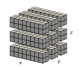
Figure 1: Decomposition of the domain in MPI into a 2D 3$\times$3 process grid.

The main advantage of PoisFFT should be its simplicity and generality. The initialization of the solver, the computation and the finalization of the solver are just three calls to the library. The arrays containing the right hand side or the solution can be a subset of a larger array. This situation arises in computational fluid dynamics when ghost cells are defined around the solution domain.

PoisFFT can solve the Poisson equation in 1, 2 and 3 dimensions with any of the boundary conditions presented in Section 2 provided all domain boundaries use the same boundary condition.

Because of practical applications in geophysical fluid dynamics, particularly in the computational fluid dynamics model CLMM (Section 5), the combination of the periodic boundary condition in the $x$ direction and Dirichlet or Neumann boundary condition in the $z$ direction is also implemented. In this case boundary condition in the $y$ direction can be periodic or identical to the condition used in the $z$ direction.

Because the parallel real 1D transform is not available in FFTW3 or PFFT we parallelized this step using a global array transpose via the subroutine MPI_Alltoallv() and local array transposes. This is necessary for the combined boundary conditions.

4 Performance evaluation

Due to the differences in the discrete Fourier transforms for different boundary conditions, the wall-clock times and the CPU times necessary for the solution of the Poisson equation depend on the boundary conditions. We chose the 3D solvers with the periodic boundary conditions and the Neumann boundary conditions on the staggered grid to test the solver with the 3D complex transform and with the 3D real transform.

All tests were performed at the cluster zapat.cerit-sc.cz at the Czech supercomputing center Cerit-SC. The computational nodes contained 2 sockets with 8-core Intel E5-2670 2.6 GHz processors and 128 GB RAM and were connected using an InfiniBand network. PoisFFT was compiled with the Intel Fortran compiler 14.1 and linked with OpenMPI 1.8.

The first test examined the strong scaling on a fixed domain with 512 points in every dimension. The same problem was solved with an increasing number of CPU cores. From the measured times in Fig. 2 it is clear that the OpenMP version, which directly calls FFTW, is considerably faster than the MPI version, which calls the PFFT wrapper over FFTW and which has to perform significant amount of message passing between processes. However, OpenMP is limited to single node on the cluster used for the computations. One can also notice a decrease of efficiency when going from 16 to 32 cores. One node has 16 cores and the expensive network memory transfers slow the computation down when more nodes are needed.

Figure 2: Strong scaling of PosFFT with $512^{3}$ points.

For the weak scaling test we used a domain discretization in which the number of points increased with the number of CPU cores. There were 256 points in each dimension per core. The complete problem size was therefore proportional to the number of cores. The results of the time measurements are in Fig. 3. They are consistent with the scaling $\mathcal{O}\left(N\ln\left(N\right)\right)$ which holds for the FFT transforms[14].

Figure 3: Weak scaling of PoisFFT with $256^{3}$ points per core.

5 Application of PoisFFT to simulation of incompressible flow

5.1 Model CLMM

Originally, PoisFFT was developed to support the atmospheric computational fluid dynamics code CLMM (Charles University Large-Eddy Microscale Model)[16]. This model simulates atmospheric flows using the incompressible Navier-Stokes equations with an eddy viscosity subgrid model.

The incompressible Navier-Stokes equations are

$$\frac{\partial\boldsymbol{u}}{\partial t}+\nabla\cdot(\boldsymbol{u}\otimes\boldsymbol{u}) =-\nabla p+\nu_{\mathrm{sgs}}\nabla^{2}\boldsymbol{u},$$ (23)

$$\nabla\cdot\boldsymbol{u} =0,$$ (24)

where $\boldsymbol{u}$ is the velocity vector, $p$ is the pressure and $\nu_{\mathrm{sgs}}$ is the eddy viscosity modeled according to Nicoud et al. [17]. Eqs. (23)–(24) do not contain an evolution equation for pressure. The model CLMM uses the projection method[1] and the 3 stage Runge-Kutta method[18]

$$\boldsymbol{u}^{(1)} =\boldsymbol{u}^{n},\>p^{(1)}=p^{n-1/2},$$ (25)

$$\frac{\boldsymbol{u}^{*}-\boldsymbol{u}^{(k)}}{\Delta t} =-\alpha_{k}\nabla p^{(k)}+\gamma_{k}\left(-\nabla\cdot(\boldsymbol{u}^{(k)}\boldsymbol{u}^{(k)})+\nu\nabla^{2}\boldsymbol{u}^{(k)}\right)+$$

$$\qquad+\zeta_{k}\left(-\nabla\cdot(\boldsymbol{u}^{(k-1)}\boldsymbol{u}^{(k-1)})+\nu\nabla^{2}\boldsymbol{u}^{(k-1)}\right)$$ (26)

$$\nabla^{2}\phi =\frac{\nabla\cdot\boldsymbol{u}^{*}}{\alpha_{k}\Delta t},$$ (27)

$$\frac{\boldsymbol{u}^{(k+1)}-\boldsymbol{u}^{*}}{\alpha_{k}\Delta t} =-\nabla\phi,$$ (28)

$$p^{(k+1)} =p^{(k)}+\phi,$$ (29)

$$\mathrm{for}\; k=1..3,\quad\mathrm{and}$$

$$\boldsymbol{u}^{n+1} =\boldsymbol{u}^{(4)},\>p^{n+1/2}=p^{(4)},$$ (30)

with the set of coefficients

$$\alpha_{1} =\frac{8}{15},\>\alpha_{2}=\frac{2}{15},\>\alpha_{3}=\frac{1}{3},$$

$$\gamma_{1} =\frac{8}{15},\>\gamma_{2}=\frac{5}{12},\>\gamma_{3}=\frac{3}{4},$$

$$\zeta_{1} =0,\>\zeta_{2}=-\frac{17}{60},\>\zeta_{3}=-\frac{5}{12}.$$ (31)

The spatial derivatives in (25)–(30) are discretized using the second order central finite differences on a staggered grid[19] with the exception of the advective terms $-\nabla\cdot(\boldsymbol{u}\otimes\boldsymbol{u})$ for which fourth order central differences are used.

In every Runge-Kutta stage first a predictor velocity field $\boldsymbol{u}^{*}$ is computed and afterward it is corrected to be divergence free. The discrete Poisson problem (27) must be solved in the corrector step, with the staggered Neumann boundary conditions on all outside boundaries except the boundaries where the periodic boundary condition for the velocity are imposed and where the periodic condition applies to the discrete Poisson equation as well. It is the task of the PoisFFT library to solve Eq. (27).

It is possible to use this model on the uniform grid to simulate certain types of complex geometries thanks to the immersed boundary method (IBM)[20], which introduces additional sources of momentum and mass inside or near the solid obstacles. In CLMM the IBM interpolations of Peller et al. [21] and the mass sources according to Kim et al. [19] are implemented.

5.2 Performance test

To evaluate the effect of CLMM we chose the test case defined by the COST Action ES1006 “Evaluation, improvement and guidance for the use of local-scale emergency prediction and response tools for airborne hazards in built environments” with a virtual city called Michelstadt which serves for validation of models for flow and dispersion in urban environments[22]. The description of the geometry and the flow validation data are available at the CEDVAL-LES website. In this paper only the velocity field is simulated for a direct comparison of the relative performance of the Poisson solver PoisFFT and other parts of the model.

The computational domain of the Michelstadt city had dimensions 1326 m $\times$ 836 m $\times$ 399 m and was discretized using a constant resolution of 3m in all directions leading to the total number of 16.3 million cells. The performance was measured for the first 100 time-steps for different parallel setups – OpenMP and MPI – with different numbers of CPU cores. The fastest configuration was used to compute the flow for 10000 s of the real scale time and the average flow and turbulence was compared to the experimental values. The performance was tested on the cluster luna.fzu.cz in the Czech national grid MetaCentrum. The computational nodes have 2 sockets with the 8-core Intel Xeon E5-2650 2.6 GHz CPU, 96 GB of RAM and are connected using an InfiniBand network.

Figure 4: Strong scaling of CLMM and PoisFFT.

The scaling of the wall-clock time for the solution of first 100 time-steps is in Fig. 4. Although the MPI version of PoisFFT is slower than the OpenMP version for the same number of CPU cores, the whole model CLMM is as fast with MPI as with OpenMP on the used nodes up to 8 threads. The OpenMP version with 16 threads is slower than the MPI version with 16 processes. CLMM appears to benefit from the improved data locality in the distributed MPI version. The relative contribution of PoisFFT to the total CLMM solution time is between 22 % – 36 % when using MPI. When using OpenMP the PoisFFT portion starts at 20 % for one and two threads and decreases for higher numbers of threads as the parallel efficiency of CLMM in OpenMP decreases. From these ratios it is clear that the efficient Poisson solver is a necessity for an efficient computation and that PoisFFT scales well enough so that it doesn’t become a bottleneck at the moderate numbers of cores used for the test.

The correctness of the computation was evaluated by comparison of the time-averaged simulated wind field with the measurements. Fig. 5 shows the comparison of the values of the velocity components in the reference points of CEDVAL-LES. An illustration of the simulated wind field at height 7.5 m above the ground is in Fig. 6.

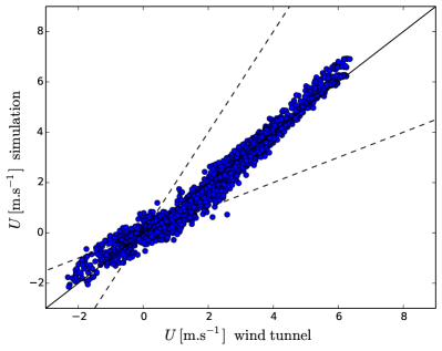
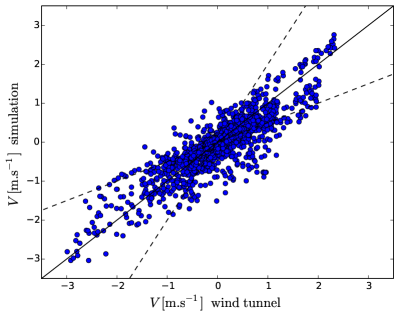
Figure 5: Scatter plots for the comparison of simulated and measured mean stream-wise ($U$) and lateral ($V$) velocity components.

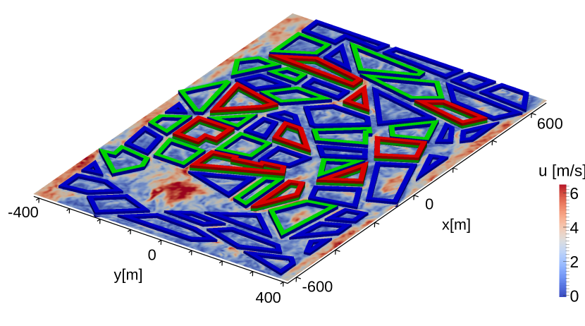
Figure 6: The Michelstadt geometry with the instantaneous field of the wind velocity magnitude at height 7.5 m above ground. The blue, green and red buildings are 15, 18 and 24 m high, respectively.

6 Conclusions

The fast Poisson solver PoisFFT is able to compute a discrete approximate solution to the Poisson equation in the pseudo-spectral or second order finite difference approximation. It is parallel using OpenMP and MPI and the parallel scaling was demonstrated to be usable for moderate numbers of CPU cores. The scaling for the number of cores in the order of thousands remain untested due to the lack of suitable hardware. The experiments of Pippig [15] with the underlying PFFT library suggest that the solver could scale even for thousands or tens of thousands of cores.

It was demonstrated that PoisFFT can be employed for the solution of the discrete Poisson equation in the projection step in an incompressible flow solver. It does not become a bottleneck at 128 cores and it is expected to scale well even further.

The library can be used from Fortran, C and C++. Interfaces to other computer languages (e.g., Python) are planned.

References

- Brown et al. [2001] D. L. Brown, R. Cortez, M. L. Minion, Accurate Projection Methods for the Incompressible Navier–Stokes Equations , Journal of Computational Physics 168 (2) (2001) 464–499, ISSN 0021-9991, URL http://www.sciencedirect.com/science/article/pii/S0021999101967154.
- Hockney [1965] R. W. Hockney, A fast direct solution of Poisson’s equation using Fourier analysis, Journal of the ACM (JACM) 12 (1) (1965) 95–113.
- Buzbee et al. [1970] B. L. Buzbee, G. H. Golub, C. W. Nielson, On direct methods for solving Poisson’s equations, SIAM Journal on Numerical analysis 7 (4) (1970) 627–656.
- Buneman [1971] O. Buneman, Analytic inversion of the five-point Poisson operator , Journal of Computational Physics 8 (3) (1971) 500–505, ISSN 0021-9991, URL http://www.sciencedirect.com/science/article/pii/0021999171900295.
- Cooley et al. [1970] J. Cooley, P. Lewis, P. Welch, The fast Fourier transform algorithm: Programming considerations in the calculation of sine, cosine and Laplace transforms , Journal of Sound and Vibration 12 (3) (1970) 315–337, ISSN 0022-460X, URL http://www.sciencedirect.com/science/article/pii/0022460X70900751.
- Wilhelmson and Ericksen [1977] R. B. Wilhelmson, J. H. Ericksen, Direct solutions for Poisson’s equation in three dimensions , Journal of Computational Physics 25 (4) (1977) 319–331, ISSN 0021-9991, URL http://www.sciencedirect.com/science/article/pii/0021999177900018.
- Swarztrauber [1977] P. Swarztrauber, The Methods of Cyclic Reduction, Fourier Analysis and the FACR Algorithm for the Discrete Solution of Poisson’s Equation on a Rectangle, SIAM Review 19 (3) (1977) 490–501, URL http://dx.//doi.org/10.1137/1019071.
- Swarztrauber [1986] P. N. Swarztrauber, Symmetric FFTs, Mathematics of Computation 47 (175) (1986) 323–346, URL http://www.ams.org/journals/mcom/1986-47-175/S0025-5718-1986-0842139-3/S0025-5718-1986-0842139-3.pdf.
- Schumann and Sweet [1988] U. Schumann, R. A. Sweet, Fast Fourier transforms for direct solution of Poisson’s equation with staggered boundary conditions , Journal of Computational Physics 75 (1) (1988) 123–137, ISSN 0021-9991, URL http://www.sciencedirect.com/science/article/pii/0021999188901027.
- Gockenbach [2006] M. S. Gockenbach, Understanding and implementing the finite element method., SIAM, ISBN 978-0-89871-614-6, URL http://www.ec-securehost.com/SIAM/OT97.html, 2006.
- Laizet and Li [2011] S. Laizet, N. Li, Incompact3d: A powerful tool to tackle turbulence problems with up to O (105) computational cores, International Journal for Numerical Methods in Fluids 67 (11) (2011) 1735–1757.
- García-Risueño et al. [2014] P. García-Risueño, J. Alberdi-Rodriguez, M. J. T. Oliveira, X. Andrade, M. Pippig, J. Muguerza, A. Arruabarrena, A. Rubio, A survey of the parallel performance and accuracy of Poisson solvers for electronic structure calculations, Journal of Computational Chemistry 35 (6) (2014) 427–444, ISSN 1096-987X, URL http://dx.//doi.org/10.1002/jcc.23487.
- Swarztrauber and Sweet [1979] P. N. Swarztrauber, R. A. Sweet, Algorithm 541: Efficient Fortran subprograms for the solution of separable elliptic partial differential equations [D3], ACM Transactions on Mathematical Software (TOMS) 5 (3) (1979) 352–364.
- Frigo and Johnson [2005] M. Frigo, S. Johnson, The Design and Implementation of FFTW3, Proceedings of the IEEE 93 (2) (2005) 216–231, ISSN 0018-9219, URL http://www.bibsonomy.org/bibtex/2744e75c05789f40e27a64bd7d40462df/jpowell.
- Pippig [2013] M. Pippig, PFFT: An extension of FFTW to massively parallel architectures, SIAMJSC 35 (03) (2013) C213–C236.
- Fuka and Brechler [2011] V. Fuka, J. Brechler, Large Eddy Simulation of the Stable Boundary Layer, in: J. Fořt, J. Fürst, J. Halama, R. Herbin, F. Hubert (Eds.), Finite Volumes for Complex Applications VI Problems & Perspectives, vol. 4 of Springer Proceedings in Mathematics, Springer Berlin Heidelberg, ISBN 978-3-642-20671-9, 485–493, 2011.
- Nicoud et al. [2011] F. Nicoud, H. B. Toda, O. Cabrit, S. Bose, J. Lee, Using singular values to build a subgrid-scale model for large eddy simulations, Physics of Fluids 23 (8) (2011) 085106, URL http://dx.//doi.org/10.1063/1.3623274.
- Spalart et al. [1991] P. R. Spalart, R. D. Moser, M. M. Rogers, Spectral methods for the Navier-Stokes equations with one infinite and two periodic directions, J. Comput. Phys. 96 (2) (1991) 297–324, ISSN 0021-9991.
- Kim et al. [2001] J. Kim, D. Kim, H. Choi, An Immersed-Boundary Finite-Volume Method for Simulations of Flow in Complex Geometries , Journal of Computational Physics 171 (1) (2001) 132–150, ISSN 0021-9991, URL http://www.sciencedirect.com/science/article/pii/S0021999101967786.
- Mittal and Iaccarino [2005] R. Mittal, G. Iaccarino, Immersed Boundary Methods, Annual Review of Fluid Mechanics 37 (1) (2005) 239–261, URL http://dx.//doi.org/10.1146/annurev.fluid.37.061903.175743.
- Peller et al. [2006] N. Peller, A. L. Duc, F. Tremblay, M. Manhart, High-order stable interpolations for immersed boundary methods, International Journal for Numerical Methods in Fluids 52 (11) (2006) 1175–1193, ISSN 1097-0363, URL http://dx.//doi.org/10.1002/fld.1227.
- Fischer et al. [2010] R. Fischer, I. Bastigkeit, B. Leitl, M. Schatzmann, Generation of spatio-temporally high resolved datasets for the validation of LES-models simulating flow and dispersion phenomena within the lower atmospheric boundary layer, in: Proceedings of Computational Wind Engineering 2010, URL ftp://ftp.atdd.noaa.gov/pub/cwe2010/Files/Papers/461_Fischer.pdf, 2010.