Resolving the shocked gas in HH 54 with Herschel

Abstract

Context. The HH 54 shock is a Herbig-Haro object, located in the nearby Chamaeleon $\tt{II}$ cloud. Observed CO line profiles are due to a complex distribution in density, temperature, velocity, and geometry.

Aims. Resolving the HH 54 shock wave in the far-infrared cooling lines of CO constrain the kinematics, morphology, and physical conditions of the shocked region.

Methods. We used the PACS and SPIRE instruments on board the Herschel space observatory to map the full FIR spectrum in a region covering the HH 54 shock wave. Complementary Herschel-HIFI, APEX, and Spitzer data are used in the analysis as well. The observed features in the line profiles are reproduced using a 3D radiative transfer model of a bow-shock, constructed with the Line Modeling Engine code (LIME).

Results. The FIR emission is confined to the HH 54 region and a coherent displacement of the location of the emission maximum of CO with increasing $J$ is observed. The peak positions of the high-$J$ CO lines are shifted upstream from the lower $J$ CO lines and coincide with the position of the spectral feature identified previously in CO (10$-$9) profiles with HIFI. This indicates a hotter molecular component in the upstream gas with distinct dynamics. The coherent displacement with increasing $J$ for CO is consistent with a scenario where IRAS12500 – 7658 is the exciting source of the flow, and the 180 K bow-shock is accompanied by a hot (800 K) molecular component located upstream from the apex of the shock and blueshifted by $-$7 $\mathrm{km\,s^{-1}}$. The spatial proximity of this knot to the peaks of the atomic fine-structure emission lines observed with Spitzer and PACS ([O i]63, 145$\mu$m) suggests that it may be associated with the dissociative shock as the jet impacts slower moving gas in the HH 54 bow-shock.

1 Introduction

Herbig-Haro objects (see e.g. Herbig, 1950; Haro, 1952) are the optical manifestations of molecular outflows (Liseau & Sandell, 1986) emanating from young stellar objects (YSOs). They reveal the shocked gas moving at the highest velocities.

A shock where the far-infrared cooling lines can be studied in detail using a very limited amount of Herschel (Pilbratt et al., 2010) time is HH 54, located in the Chamaeleon II cloud. At a distance of only 180 pc (Whittet et al., 1997) it is close enough to be spatially resolved with Herschel. The source of the HH 54 flow is, however, a matter of debate. Several nearby IRAS point sources have been proposed as the exciting source (see e.g. Caratti o Garatti et al., 2009; Bjerkeli et al., 2011, and references therein), but the issue remains essentially unsettled. Previous observations have shown that observed CO line profiles, from $J_{\rm{up}}$ = 2 to 10, are due to a complex distribution in temperature, density, velocity, and geometry (Bjerkeli et al., 2011). In particular, these observations revealed the presence of a spectral bump, tracing a distinctly different gas component than the warm gas ($\sim$200 K) responsible for the bulk part of the CO line emission.

In this paper, we present spectroscopic observations (50 – 670 $\mu$m) of CO at a high spatial resolution acquired with PACS (Poglitsch et al., 2010) and SPIRE (Griffin et al., 2010). We also present velocity resolved observations of the CO (15$-$14) line and the CO (3–2) line obtained with HIFI and APEX, respectively. These datasets are analysed in conjunction with previously published CO and H₂ data acquired with Herschel and Spitzer, providing valuable information on the kinematics, morphology, and physical conditions in the shocked region.

2 Observations

The OT2 Herschel data presented here were observed in PACS range spectroscopy mode in July 2012, SPIRE point spectroscopy mode in December 2012, and HIFI single pointing mode in September 2012. The observations were centred on HH 54 B, $\alpha_{2000}$ = 12^h55^m50$\stackrel{{{}^{\rm s}}}{{{}_{\bf\cdot}}}$3, $\delta_{2000}$ = –76^∘56^′23^′′ (Sandell et al., 1987), and covered the wavelength region $\sim$50 – 670 $\mu$m. The PACS receiver includes 5 by 5 spatial pixels (spaxels), each covering a region of 9.4^′′ by 9.4^′′. The SPIRE spectrometer has a field of view of 2$\stackrel{{\scriptstyle\prime}}{{{}_{\bf\cdot}}}$6 and full spatial sampling was used to allow the determination of the position of the emission maximum to a high accuracy. In this observing mode, the Beam Steering Mirror is moved in a 16-point jiggle to provide complete Nyquist sampling of the observed region. In both the PACS and SPIRE observations, each emission line is unresolved in velocity space. The velocity resolved spectrum of the CO (15$-$14) line was observed with HIFI (de Graauw et al., 2010), where the full width half maximum (FWHM) of the beam is 12^′′. The channel spacing is 500 kHz (0.09 $\mathrm{km\,s^{-1}}$ at 1727 GHz) and the spectrum was converted to the $T_{\rm mb}$ scale using a main-beam efficiency of 0.76. The data were reduced in IDL and Matlab.

The CO (3$-$2) observations, where the FWHM of the beam is 18^′′, were acquired with the APEX-2 receiver in March 2012. A rectangular region (80^′′ $\times$ 80^′′) centred on HH 54 B was observed and the channel spacing is 76 kHz (0.06 $\mathrm{km\,s^{-1}}$ at 346 GHz). The data reduction was performed in Matlab and the spectrum was converted to the $T_{\rm{mb}}$ scale using the main beam efficiency 0.73.

For the analysis, we also make use of already published CO data (Bjerkeli et al., 2011) and H₂ data (Neufeld et al., 2006). For the observational details we refer the interested reader to those publications.

3 Results

Table 1: Total CO line fluxes and FWHM from the Gaussian fitting.

Transition	Frequency	Line flux	FWHM
	(GHz)	($10^{-13}$ erg $\rm{s}^{-1}$ cm-2)	(′′)
4 – 3	461.041	1.49 $\pm$ 0.77	52.8 $\pm$ 6.9
5 – 4	576.268	4.21 $\pm$ 1.07	52.8 $\pm$ 3.4
6 – 5	691.473	6.20 $\pm$ 0.99	45.6 $\pm$ 1.8
7 – 6	806.652	9.84 $\pm$ 1.41	47.3 $\pm$ 1.7
8 – 7	921.800	11.3 $\pm$ 1.47	45.3 $\pm$ 1.5
9 – 8	1036.912	8.71 $\pm$ 1.20	31.3 $\pm$ 1.0
10 – 9	1151.985	8.36 $\pm$ 1.24	30.8 $\pm$ 1.1
11 – 10	1267.014	7.05 $\pm$ 1.33	30.1 $\pm$ 1.4
12 – 11	1381.995	6.36 $\pm$ 1.34	30.8 $\pm$ 1.6
13 – 12	1496.923	4.76 $\pm$ 1.44	28.8 $\pm$ 2.1
14 – 13	1611.794	5.07 $\pm$ 4.80	26.3 $\pm$ 6.5
15 – 14	1726.603	4.55 $\pm$ 3.88	21.0 $\pm$ 4.5
16 – 15	1841.346	4.03 $\pm$ 2.99	22.5 $\pm$ 4.3
17 – 16	1956.018	2.76 $\pm$ 2.95	23.1 $\pm$ 6.2

Figure 1 shows the spectrum obtained with PACS and SPIRE towards the position closest to HH 54 B, i.e. the central spaxel for the PACS observations.

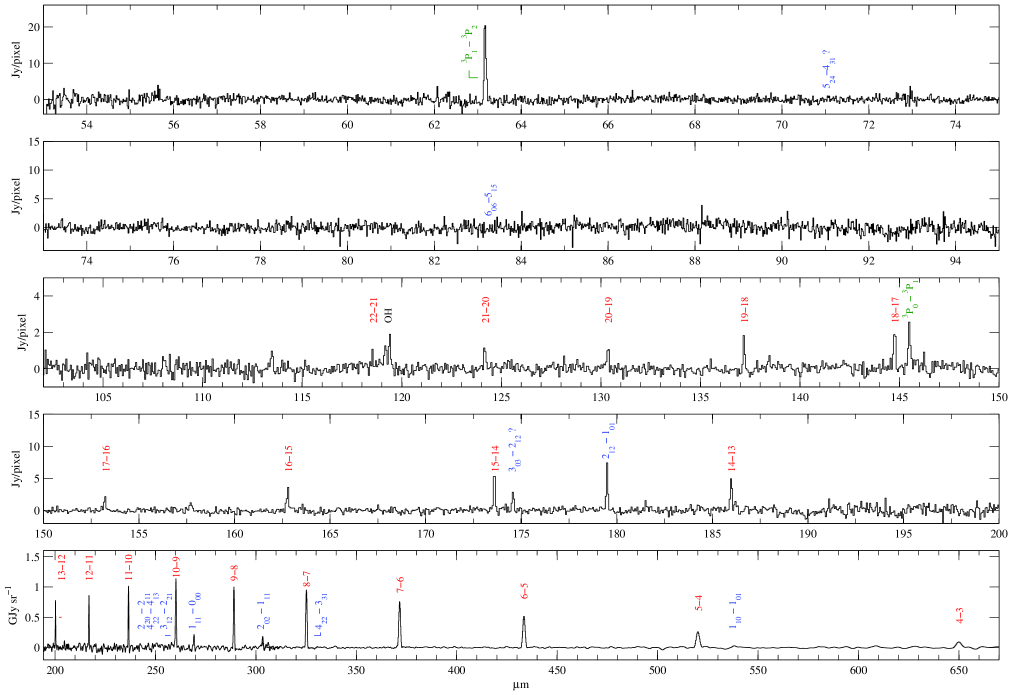
Figure 1: Upper four panels: PACS spectrum towards the central spaxel. Only lines that are detected with a signal-to-noise ratio greater than 3 somewhere in the mapped region (not necessarily the central spaxel) are marked as a detected line. Only upper and lower state energy levels are indicated for clarity. Lower panel: Same as the other panels but for the SPIRE spectrum towards the central region. The [O i] lines are marked in green, the H₂O lines in blue and the CO lines in red. In this figure, there are different units for the PACS and SPIRE observations and no continuum subtraction has been made.

No significant continuum emission is detected, however, all CO rotational emission lines from $J_{\rm{up}}=4$ to 22 are detected at the 5 $\sigma$ level (line flux) or higher in at least one position in the observed region. The CO line fluxes are consistent with the fluxes measured with ISO (Nisini et al., 1996; Giannini et al., 2006), within the error bars. The total line fluxes are calculated by fitting Gaussians to each emission map (see Fig. 3 and Sec. 4) and are presented in Table 1. The higher-$J$ CO lines ($J_{\rm{up}}>$ 17) are excluded from this table due to the few positions where a 5 $\sigma$ detection is reached. In addition to the CO ladder, one OH line, the [O i] lines at 63 and 145 $\mu$m, and several H₂O lines are detected. The water emission from HH 54 is further discussed in a forthcoming paper (Santangelo et al., 2014a). [O iii] is not detected, nor is [N ii] or [C ii], however, there is a feature (158 $\mu$m) at the 2.5 $\sigma$ level. The emission from all lines is confined to the HH 54 region. A bump-like feature (also discussed in Bjerkeli et al., 2011) is clearly detected in the CO (3$-$2) spectrum and likely also in the CO (15$-$14) spectrum. In Fig. 2, these two lines are shown, compared to the CO (10$-$9) spectrum (Bjerkeli et al., 2011). The blue-shifted extent is the same for all three lines, and the peak velocity of the bump is within 2 $\mathrm{km\,s^{-1}}$ for the three lines. The CO (3$-$2) observations suffered from contamination close to the cloud LSR velocity. This is of minor importance, however, for the analysis presented in this paper.

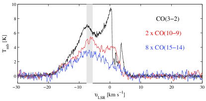
Figure 2: Comparison between the CO (3$-$2), CO (10$-$9), and CO (15$-$14) spectra. The latter two have been scaled for clarity. The peak velocity of the bump is within 2 $\mathrm{km\,s^{-1}}$ for all three lines (shaded area).

4 Discussion

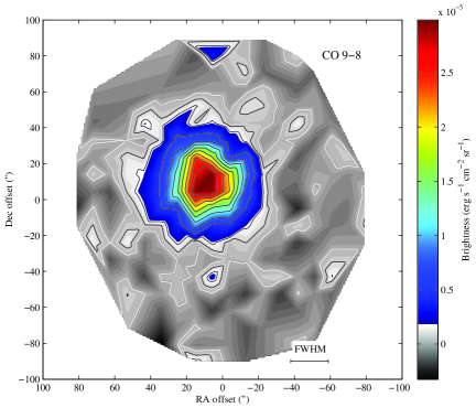
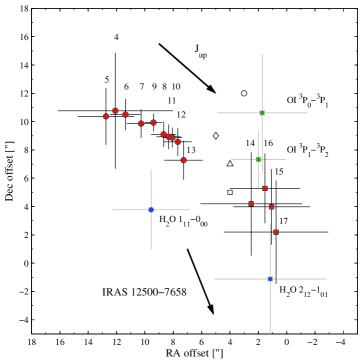
Figure 3: Left panel: The CO (9–8) line emission obtained with SPIRE. The coloured contours show where the signal-to-noise ratio is higher than 5, the black line indicate the 3$\sigma$ level and the white line the 1$\sigma$ level. The FWHM of the SPIRE beam is indicated in the lower right corner of this figure. Right panel: The red (CO), blue (H₂O) and green ([O i]) markers show the location of the emission maximum with error bars from the Gaussian fit. The open square, circle, triangle and diamond show the peak positions of the fine-structure emission lines [Ne ii] 12.8 $\mu$m, [Fe ii] 26 $\mu$m, [S i] 25 $\mu$m, and [Si ii] 35 $\mu$m lines, respectively (Neufeld et al., 2006, Fig. 3). The arrows indicate the direction of increasing $J_{\rm{up}}$ for CO and the direction to IRAS 12500–7658. The quantum numbers (only $J_{\rm{up}}$ for CO) are also shown in the figure. Angular offsets are given relative to the position of HH 54 B.

4.1 Structure of the shock

Even though the observed lines are only marginally resolved spatially, we can still (thanks to the high signal-to-noise ratio) determine the position of each emission maximum to a high accuracy. We therefore fit 2D Gaussians to each CO map and measure the position of the maximum. The result is a coherent displacement with increasing $J$ (see Fig. 3). In this figure, the peak position of the two [O i] lines and the two H₂O lines that are detected at a sufficient signal-to-noise ratio are also plotted. The CO (9–8) map obtained with SPIRE is shown as well, as an illustrative example. Since the lines are observed simultaneously with each instrument, the measurement of the spatial shift as a function of $J$ is robust. One explanation to this shift, since the shock is oriented almost along the line of sight (Caratti o Garatti et al., 2009), could be different portions of the shocked surface having different temperatures and/or densities. A hot molecular knot (traced by high-$J$ CO) on this surface would always appear projected upstream with respect to the bow outer rim (i.e. with respect to the region where the low-$J$ CO lines peak). The observed gradient in excitation is, however, consistent with the scenario that was presented in Bjerkeli et al. (2011), i.e. the centroids of the high-$J$ CO lines coincide spatially with the bump-like feature detected in the CO (10$-$9) line, discussed in that paper (their Fig. 5). These authors suggested that the bump traces an unresolved hot, low-density component and this is likely the cause of the observed displacement with increasing $J$ (Sec. 4.2). If IRAS 12500-7658 is the exciting source, this component appears located upstream of the bow-shock in projection. The opposite trend is observed in other sources (see e.g. Santangelo et al., 2014b). On the other hand, the situation is morphologically reminiscent to the L1157-B1 case (Benedettini et al., 2012). The high-$J$ CO emission peak is also in that object shifted upstream by about 10^′′ from the outer bow-shock rim delineated by lower excitation lines. In both sources, this high-$J$ CO seems spatially associated with ionic fine structure lines such as [Fe ii] and [Ne ii] (Neufeld et al., 2006) and [O i] upstream of the bow-shock (see Fig. 3). The bright and compact ionic emission in HH 54 and L1157-B1 is understood as tracing the dissociative and ionizing shock, where the jet suddenly encounters the slow-moving ambient shell (Neufeld et al., 2006; Benedettini et al., 2012). Thus, the possibility exists that the high-$J$ CO emission, and the associated bump spectral feature, are produced in a region related to the reverse shock (e.g. Fridlund & Liseau, 1998). The apparent association of high-$J$ CO emission with a strongly dissociative shock, both in HH 54 and in L 1157-B1, would imply that either the jet material is already partly molecular, or that molecule reformation is efficient. Testing these interpretations clearly calls for further modelling work, that lies outside the scope of the present paper.

4.2 Observed line profiles

To check whether a low density, hot component can give rise also to the observed bump in the line profiles, we have updated the model presented in Bjerkeli et al. (2011). The models discussed there, were limited by the 1D+ geometry of the ALI code, used for the calculation of the radiative transfer. In this paper, we instead use the accelerated Monte-Carlo code LIME (Brinch & Hogerheijde, 2010), that allows the full 3D radiative transfer to be calculated. The LIME code does not put any constraints on the complexity of the models that can be constructed. Nevertheless, we have chosen to keep it simple for clarity. We therefore, again, compute the radiative transfer for a model that is observed from the front, but in this case with a small inclination angle with respect to the line of sight, i.e. 25^∘ (Caratti o Garatti et al., 2009). We use the density ($n$($\mathrm{H_{2}}$) = $10^{5}$ cm^-3) and temperature ($T_{\rm{kin}}\leavevmode\nobreak\ =\leavevmode\nobreak\ 180\leavevmode\nobreak\ \rm{K}$) inferred from the $\chi^{2}$ analysis presented in Bjerkeli et al. (2011, their Sec. 4.3). The difference between the model presented in that paper and the model presented here, is mainly the presence of a slightly under-dense ($n$($\mathrm{H_{2}}$) $\simeq$ $10^{4}$ cm^-3), hot ($T_{\rm{kin}}$ $\simeq$ 800 K) component that is located upstream of the bow-shock.

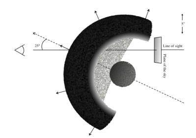
Figure 4: A 3D view of the model described in the text. The colours represent the magnitude of the velocity field, increasing from the inside (light grey) of the bow-shock component to the outside (dark grey). The direction of the velocity field is indicated with arrows and the motion of the Herbig-Haro object is indicated with a dashed line. The hot component, producing the bump spectral feature is located at the centre of the model and the inclination with respect to the line of sight is 25^∘. A cut has been made through the top of the model for clarity.

The size of the emitting region is set to 7^′′ (Neufeld et al., 2006), the velocity is set to $\upsilon_{\rm LSR}$ = –7 $\mathrm{km\,s^{-1}}$, and the velocity dispersion to 5 $\mathrm{km\,s^{-1}}$. The bow-shock is again represented by an expanding shell at constant density and temperature. In the model presented here, however, the rear side of the sphere and the central blackbody source (Bjerkeli et al., 2011) are removed, and the shell thickness has been decreased by a factor of two, i.e. $\Delta s$ =  2.5$\,\times\,10^{15}$ cm (see Table LABEL:table:limemodel and Fig. 4 for details). 500 000 grid points are used in the calculation.

In Fig. 5, we present the CO (3$-$2), CO (10$-$9), and CO (15$-$14) line profiles observed towards HH 54, together with the model that fit the observations best. Given the increased number of free parameters, and because a full chi-square analysis is impracticable, we use by-eye comparison when fitting the lines. From Fig. 5, it is clear that the observed lines, in essence, can be reproduced using this simplistic 3D model of an expanding bow-shock with a slightly under-dense and hot component. The spatial shift, due to the inclination ($\sim$5^′′), between the centroids of the modelled low-$J$ and high-$J$ CO lines, can to a great extent explain the observed displacement with increasing $J_{\rm{up}}$ (Fig. 3). We were not able to reproduce the line shapes, when using a high density and low temperature for the bump component. Why the CO (15$-$14) line (where the line strength is completely accounted for by the hot component in the model) has a similar line width as the low-$J$ CO lines is, however, at present not fully understood. The inferred CO column density is 1$\,\times\,10^{16}$ cm^-2, for the low-temperature component. The H₂ column density of 1$\,\times\,10^{20}$ cm^-2, is consistent with the column density obtained from a population diagram analysis using Spitzer H₂ data (Neufeld et al., 2006). From inspection of these diagrams, the S(0) line and the S(1) line seem to trace gas at lower excitation (as in the case of VLA 1623, Bjerkeli et al., 2012). Taking only these two lines into account (where $E_{\rm{up}}/\rm{k}<1020\leavevmode\nobreak\ K$), and assuming an ortho-to-para ratio of 3, we estimate the H₂ column density in the region to lie in the range 0.5 – 1$\,\times\,10^{20}$ cm^-2. Taking the uncertainties of the above values into account, the assumed CO/H₂ ratio of 1$\,\times\,10^{-4}$, for the low-temperature component, is estimated to be correct to within a factor of 4.

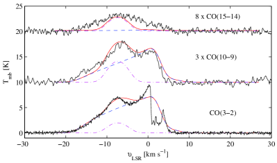
Figure 5: The observed CO (3$-$2), CO (10$-$9), and CO (15$-$14) spectra compared with the best-fit two-component model (red). The upper two lines have been shifted upwards and the foreground emission and absorption is not included in the model. The contributions from the bump and the expanding shell have been calculated separately and are indicated with dash-dotted purple and dashed blue lines, respectively.

5 Conclusions

The FIR spectrum towards HH 54 has been observed successfully. CO lines from $J_{\rm{up}}$ = 4 to 22, 9 H₂O lines, and the [O i] 63 $\mu$m and [O i] 145 $\mu$m lines, are detected. The CO transitions observed with SPIRE and PACS show a coherent displacement in the emission maximum with increasing $J$. The gradient goes in the direction of the source IRAS 12500 – 7658, which has been proposed to be the exciting source of the HH 54 flow. We interpret this as an under-dense, hot component present upstream of the HH 54 shock wave. The peak positions of the high-$J$ CO lines are spatially coincident with the peaks of [O i], [Ne ii], [Fe ii], [S i], and [Si ii]. Non-LTE radiative transfer modelling, taking the full 3D geometry into account can explain the observed CO line profile shapes and the spatial shift between the various CO lines. The CO/H₂ ratio for the low-temperature gas is estimated at $\sim$$10^{-4}$.