Tomography by noise

Abstract

We present an efficient and robust method for the reconstruction of photon number distributions by using solely thermal noise as a probe. The method uses a minimal number of pre-calibrated quantum devices, only one on/off single-photon detector is sufficient. Feasibility of the method is demonstrated by the experimental inference of single-photon, thermal and two-photon states. The method is stable to experimental imperfections and provides a direct, user-friendly quantum diagnostics tool.

Introduction. - Ultimately, the quantum tomography is the most comprehensive tool available for a researcher. Indeed, by inferring the quantum state we have a possibility to predict results of any possible measurement. From its birth in 1989 vogel , quantum tomography has made an enormous progress all ; special . Now even such fragile quantum objects as “Schrödinger cats” made of photons are diagnosed and reconstructed cats . However, the most precise tool requires the most precise tuning. Generally, the quantum reconstruction schemes require precise calibration of the measurement set-up together with minimization of noise and losses. For example, one of the most established tomographic tools for electromagnetic field states, the quantum homodyne tomography requires more than $50\%$ overall detection efficiency dariano95 . Also, rather low respective phase noise of the probe and signal fields is essential for the scheme to work.

In this Letter we present a quantum tomography scheme that actually relies on the noise to collect data sufficient for the state reconstruction. Furthermore, the data is collected by using merely one on/off detector, where the ability to distinguish the number of the input photons is not required. The essence of the scheme is simple: the signal mixed with the thermal noise impinges on the detector. Varying intensity of the noise, we can build up the set of measurements sufficient for the inference of diagonal elements of the signal density matrix. The reconstruction can be done even for quite low detection efficiencies on the level of 10$\%$ . An important feature of our scheme is the minimization of resources. Even the simplest of the conventional schemes using one on/off avalanche photo-detector still requires a number of pre-calibrated absorbers or beam-splitters mog98 . With increasing signal intensity, this number increases dramatically. The schemes based on time-multiplexing or space-multiplexing similarly involve a considerable amount of pre-calibration loop ; timemultiplex . Additionally, they assume that the signal does not contain photon number contributions beyond the number of multiplexing channels. In contrast, in our scheme the detector itself can be used to determine the temperature of noise, thus avoiding the necessity to have any other pre-calibrated devices. Moreover, there is no restriction to the low dimensional Hilbert space corresponding to low input photon number pre-defined by the detector. Our scheme can be generalized to enable a complete reconstruction of the signal state density matrix by mixing the signal with the coherent field.

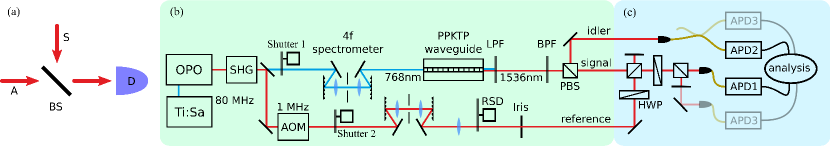
Figure 1: (a) The sketch of the measurement scheme: the signal A is mixed with the probe S on the beam-splitter (BS) and impinges on the bucket detector D. (b) State preparation setup. Pulsed light at telecom wavelengths is generated in a Ti:Sapph pumped optical parametric oscillator (OPO) and frequency doubled by second harmonic generation (SHG). Part of the light is separated for later use as a reference field. The repetition rate of the reference is lowered by an acousto-optical modulator (AOM). The 4-f spectrometer tailors the spectral width of the pump beam to achieve spectral decorrelation. The PDC state is generated inside the periodically poled KTP waveguide. The pump is separated by a long pass filter (LPF). A bandpass filter (BPF) is used to suppress background outside the PDC spectrum. Finally signal and idler are separated at a polarizing beam splitter (PBS). The reference field is also spectrally tailored by a 4-f setup. Pseudo-thermal light is generated by a rotating speckle disk (RSD) followed by irises. (c) Measurement setup. Signal and reference are overlapped at a PBS-HWP-PBS combination, which effectively constitutes a variable BS adjusted to a splitting ration of $90/10$. The power of the reference is controlled by the first HWP. Probed signal and idler are coupled into single mode fibers and impinge onto two avalanche photo diodes (APDs) (Id Quantique id201 at a repetition rate of 1MHz with a gate width of about 2.5ns). A third APD is used either in the idler beam to herald two photon states or in the second output port of the variable BS to estimate the mode overlap between signal and reference by Hong Ou Mandel interference.

The scheme. - We first demonstrate the feasibility of our scheme in its simplest configuration. The goal is to infer diagonal elements of the signal density matrix, $\rho_{mm}$, in the Fock-state basis, $|m\rangle$. The probability of registering a signal is generally given as

$$p_{j}=\sum\limits_{m=0}^{N}\Pi_{jm}\rho_{mm},$$ (1)

where the elements $\Pi_{jm}=\langle m|\Pi_{j}|m\rangle$ are related to the $j$th element of positive valued operator measure (POVM), $\Pi_{j}$, which describes a measurement performed on the signal. $N+1$ is the dimension of the subspace of all possible signal states. We have only one on/off detector and we use different thermal probe states to generate different POVM elements. Let us suppose that the probe completely overlaps with the signal at the detector, which has a detector efficiency $\eta$. If we now register “no click” events, we obtain POVM operator matrix elements for such a measurement perina ; rockower :

$$\Pi_{jm}=y_{j}(1-y_{j}{\eta})^{m},$$ (2)

where $y_{j}={1}/(1+\eta{n}_{j})$ and $n_{j}$ is the mean photon number of the probe thermal state (TS). The matrix with elements $(x_{j})^{m}$ is always non-degenerate for $N+1$ different values of $x_{j}$ and $m=0,1\ldots N$ (it is the Vandermonde matrix horn ). Since we can represent the system (1) as $p_{j}/y_{j}=\sum\limits_{m=0}^{N}(1-y_{j}{\eta})^{m}\rho_{mm}$, it means that using TS probes provides us with measurements, which should provide enough information to reconstruct elements $\rho_{mm}$. To collect the necessary data, only one pre-calibrated on/off detector is needed and it is sufficient to change the probe arbitrarily. When the signal is blocked, the average number of photons, $n_{j}$, in the probe can be measured.

In practice, instead of the simplest scheme (2), we have mixed the probe with the signal using a beam-splitter (BS) (see the scheme (a) in Fig.(1)). For two imperfectly overlapping fields, the signal $a$ and the probe $b$, interfering on BS and afterwards impinging on the detector, the probability to register “no click” is given by laiho :

$$p_{j}={\rm Tr}\{:\exp\{-\eta(Ta^{\dagger}a+(1-T)b^{\dagger}b+$$

$$x(a^{\dagger}b+b^{\dagger}a))\}:\rho\sigma_{j}\},$$ (3)

where $a^{\dagger}$, $a$ and $b^{\dagger}$, $b$ are the creation and annihilation operators of signal and probe modes; $\sigma_{j}$ is the density matrix of the $j$th probe field; $T$ is the transmissivity of BS; $x=\sqrt{\mu T(1-T)}$, $\mu$ is the overlap parameter; $::$ denotes the normal ordering operator. For the perfect overlap, Eq.(3) results in a straightforward relation:

$$\Pi_{jm}=\sum\limits_{n,k,l=0}^{N}(1-\eta)^{k}\sigma_{nj}|U^{kl}_{mn}|^{2}.$$ (4)

Quantities $\sigma_{nj}=(n_{j})^{n}/(1+n_{j})^{n+1}$ are diagonal matrix elements of the $j$th probe TS. The operator $U$ describes the rotation performed by BS. It has the following matrix elements in the Fock-state basis:

$$U^{kl}_{mn}=\sqrt{k!l!m!n!}\sum\limits_{g=0}^{k}\sum\limits_{h=0}^{l}\frac{t^{g+h}r^{k+l-g-h}(-1)^{k-g}}{g!h!(k-g)!(h-l)!}\times$$

$$\delta_{m,l+g-h}\delta_{n,k+h-g}.$$ (5)

Here $t=\sqrt{T}$ and $r=\sqrt{1-T}$. For the zero-temperature noise, $n_{j}=0$, Eq.(4) gives

$$p_{\rm{signal}}=\sum\limits_{k=0}^{N}(1-T\eta)^{k}\rho_{kk}.$$ (6)

Now let us represent the probe TS as a mixture of coherent states, $|\alpha\rangle$, perina : $\sigma_{j}=\frac{1}{\pi n_{j}}\int d^{2}\alpha\exp\{-|\alpha|^{2}/n_{j}\}|\alpha\rangle\langle\alpha|$. In the case of the perfect overlap, $p_{j}$ for probe TS can be expressed through the probability of “no clicks” for the coherent probe (given in Ref.laiho ):

$$p_{j}=\frac{1}{\pi{n}_{j}}\int d^{2}\alpha\exp\{-|\alpha|^{2}/n_{j}\}\times$$

$$\langle:\exp\{-\eta T(a^{\dagger}+\nu\alpha^{*})(a+\nu\alpha)\}:\rangle_{a},$$ (7)

where $\nu=\sqrt{(1-T)/T}$. Notice, that this formula is equivalent to the expression for $p_{j}$ given by POVM elements (4) for $N\rightarrow\infty$. The POVM elements for an imperfect overlap can be derived representing Eq.(3) for $p_{j}$ for the probe TS in the form similar to Eq.(7):

$$p_{j}=\frac{{\bar{n}}_{j}}{\mu n_{j}}\frac{1}{\pi{\bar{n}}_{j}}\int d^{2}\alpha\exp\{-|\alpha|^{2}/{\bar{n}}_{j}\}\times$$

$$\langle:\exp\{-\eta T(a^{\dagger}+\nu\alpha^{*})(a+\nu\alpha)\}:\rangle_{a}.$$ (8)

The quantity ${\bar{n}}_{j}={\mu n_{j}}/(1+(1-\mu)(1-T)\eta n_{j})$. Comparing the expression (8) with Eqs. (7), (4) for the perfect overlap, we obtain the relation for the POVM elements in case of the imperfect overlap:

$$\Pi_{jm}^{\rm overlap}=\frac{{\bar{n}}_{j}}{\mu n_{j}}\sum\limits_{n,k,l=0}^{N}(1-\eta)^{k}{\bar{\sigma}}_{nj}|U^{kl}_{mn}|^{2},$$ (9)

where ${\bar{\sigma}}_{nj}$ are the diagonal matrix elements of TS with the average number of photons ${\bar{n}}_{j}$. Eq. (9) points to a number of important conclusions. First of all, for the zero overlap, the “modified” average number of photons is also zero, ${\bar{n}}_{j}=0$. As follows from Eqs.(6), (9), the resulting “no click” probability factorizes, $p_{j}(\mu\rightarrow 0)\rightarrow{p_{\rm{signal}}}p_{\rm{term}}$, where $p_{\rm{term}}=1/(1+(1-T)\eta n_{j})$ is the “no click” probability for the probe TS with the vacuum instead of the signal. For a weak probe, when $(1-\mu)(1-T)\eta n_{j}<<1$, the actual situation can be modelled by having two probe modes, the one completely overlapping with the signal with average number of photons equal to $\mu n_{j}$, and the non-overlapping one with average number of photons equal to $(1-\mu)n_{j}$. When the probe is strong, $(1-\mu)(1-T)\eta n_{j}>>1$, part of the probe actually interfering with the signal remains constant, ${\bar{n}}_{j}\approx\mu/(1-\mu)(1-T)\eta$. In other words, too strong probe will wash out effects of interference and destroy a possibility to reconstruct the signal. The optimal regime is the moderate levels of the probe TS.

It should be noticed that our set-up can be easily generalized for the complete state reconstruction. Coherently shifting the signal with the amplitude $\alpha$, one can reconstruct the set of following quantities: $\langle m|D(\alpha)\rho D^{\dagger}(\alpha)\ |m\rangle$, where the coherent shift operator is $D(\alpha)=\exp\{\alpha a^{\dagger}-\alpha^{*}a\}$. For an $N$-dimensional density matrix of the signal, it is sufficient to have $N$ different settings of the coherent shift and $N$ TS to infer the complete density matrix (for the procedure see, for example, Refs.ourprl2006 ). To realize this generalization with our set-up, apart from the one additional fixed BS, one needs only to have a pre-calibrated phase-shifter to change a relative phase of the added coherent field.

Setup. - For the signal state generation we employ a type-II parametric downconversion (PDC) source in a periodically poled KTP waveguide. The source is characterized in detail in harder_optimized_2013 . It produces spectrally nearly decorrelated PDC states such that heralded states have a high purity above $80\%$. Furthermore, being a waveguide source, it allows for efficient coupling into single mode fibers. A scheme of the full setup is shown in Fig. 1. To simulate a noise source with TS photon number statistics, we generate pseudo-thermal light using a rotating speckle disk. For each position of the speckle disk, a random interference pattern is created. After spacial filtering by irises and the final fiber incoupling, the intensity shows an exponential, hence thermal, probability distribution. We verify the thermal statistics by measuring the mean photon number for different positions of the disk as well as by the second-order correlation function $g^{(2)}$. We obtain $g^{(2)}>1.9$, whereas a value of $g^{(2)}=2$ corresponds to perfect thermal statistics and $g^{(2)}=1$ to Poissonian statistics. The remaining coherent part is thus very small and can be neglected. The calibration parameters of our scheme are the mode overlap between signal and probe $\mu$ and the overall efficiency $\eta$. To determine the mode overlap, we adjust our variable beam splitter to 50/50 and measure a Hong-Ou-Mandel dip. The overlap is calculated from the visibility of the dip as described in Kaisa_HOM to be $\mu=0.45$. The decrease from unity comes possibly from a spectral mismatch in the 4-f setup or a spacial mismatch while coupling into the fiber. The detection efficiency is measured using the Klyshko scheme klyshko from which we obtain $\eta=0.15$. To generate a set of probe states, we rotate a HWP (see Fig. 1) and measure the mean photon numbers $n_{j}$ from counts in APD1 with a physically blocked PDC beam.

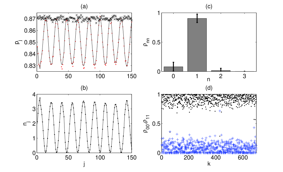
Figure 2: Reconstruction of the heralded single-photon state for the scheme parameters $\eta=0.15$ and $\mu=0.45$. $10^{7}$ PDC pulses were used for each value of the reference field intensity (a). Dots show experimentally collected data for the number of “no clicks” with respect to the total number of pulses for the signal overlapped with the reference beam. The oscillating behavior comes from the fact that a HWP is used to change the reference beam power at each measurement point. Crosses depict the same probability of “no clicks” on the APD for the signal alone; solid line shows probabilities estimated by Eq.(9) for the result shown in Fig. 2(c). (b) Average number of thermal photons, $n_{j}$, of the probe for the data of (a). (c) Experimentally inferred $\rho_{nn}$ of the heralded single-photon state. (d) Experimentally estimated values of vacuum (crosses) and single-photon (dots) components of the signal obtained via bootstrapping the data shown in the panel (a).

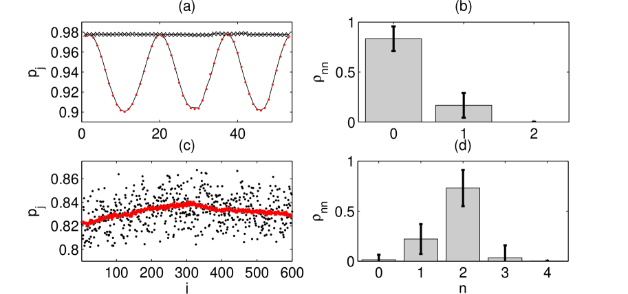
Figure 3: (a, b) Reconstruction of the thermal state. (a) Dots show experimentally collected data for the number of “no clicks” with respect to the total number of pulses for the unheralded signal overlapped with the probe. Crosses depict the relative number of “no clicks” on the APD for the signal alone; solid line shows probabilities estimated by Eq.(9) for the average reconstruction result shown in Fig. 3 (b). (c, d) Reconstruction of the two-photon state. (c) Dots show experimentally collected data for the number of “no clicks” with respect to the total number of pulses for the heralded two-photon signal without the reference; solid line shows experimentally collected data for the number of “no clicks” in respect to the total number of pulses for the heralded single-photon signal without the reference. (d) Experimentally inferred $\rho_{nn}$ of the heralded two-photon state obtained accounting for the efficiency drift. The scheme parameters are as in Fig. 2; 600 different settings of the reference field were taken.

Results. - Fig. 2 shows the results of reconstruction for the heralded single-photon state generated by the scheme depicted in Fig. 1. Total 150 measurement points were used for the inference. The reconstruction was done using least-square estimation with non-negativity constraints our njp 2013 . The detection efficiency $\eta=0.15$ and the overlap $\mu=0.45$ were assumed. Fig. 2 (d) visualizes the estimated values of vacuum and single-photon components of the signal obtained via bootstrapping the data bootstrap . Our reconstruction procedure for the single-photon state gives the following value of the single-photon component $\rho_{11}\approx 0.905\pm 0.07$. This estimate conforms well with the result of the recent work harder_optimized_2013 where the same source was used, demonstrating high quality of the reconstruction. Also, quite similar result was obtained with the same source using the ”data pattern” reconstruction method arxivzdenek . Fig. 3 shows experimentally obtained data for the heralded two photon state and the thermal state pdc thermal . In Fig. 3(a) only a part of the measured data is shown. Here, when varying the probe intensity, 600 different values of reference field intensity were taken. The average photon-number distribution shown in Fig. 3 (b) is close to the thermal with the average number of photons equal to $0.17$. Relatively large values of variances might be explained by the fact that the signal field intensity was significantly higher in difference to the case shown in Fig. 2. As a consequence, parameters of the measurement set-up were not as stable. In particular, the detection efficiency was drifting, so that an efficiency drift of about $15\%$ was registered. This deviation might result from a drift in the fiber incoupling efficiency due to instabilities of the setup over the measurement time. The data for the heralded two-photon state is affected in a similar way as can be clearly seen also in Fig. 3 (c). Here we show experimental data for both heralded two-photon signal (dots) and heralded single-photon signal (solid line) not mixed with the reference. One of the powerful features of our method is the possibility to account for these deviations, by assuming varying efficiency. For the estimation of the detection efficiency, we need to use the data for the signal state not mixed with the reference. For example, if we take the single-photon state, use Eq. (6) and the experimentally measured probability $p_{\rm signal}$ as shown in Fig. 2, we can compute the actual values of $\eta$. The drift in the detection efficiency $\eta$ is reflected in the varying value of $p_{j}$ for the heralded single-photon signal without the reference, as depicted by the solid (red) line in Fig. 3 (c). Ideally, this should be a straight line, as it is approximately for the data set with the low field intensity, used for the single-photon state reconstruction ($p_{j}$ in Fig. 2 (a), solid line). For the data set with the higher field intensity, as used for the two-photon reconstruction, this is not the case anymore (Fig. 3 (c)). To account for this, we incorporated the calculated actual efficiency values in the expression for the POVM elements (9) when inferring $\rho_{nn}$ for the generated two-photon state (Fig. 3 (d)). The obtained results for the two-photon signal are quite similar to obtained recently with the same source using the ”data pattern” method arxivzdenek . It should be emphasized that deviations of obtained data do not lead to reconstruction artifacts in our scheme. For example, the vacuum component of the reconstructed signal remains very low despite a rather noisy character of the data. Also, the result of reconstruction does unambiguously show that despite low efficiencies of the detection, the scheme produces states with large two-photon component. All these feature are preserved even if no correction for varying detection efficiency is performed for the two-photon state (Fig. 3 (d)), although the relative errors are much higher then.

Conclusions. - We have demonstrated both theoretically and experimentally that reconstruction by noise is indeed feasible and provides a lucid, robust tomographic tool. By merely mixing the signal with the thermal noise and measuring statistics of the resulting field on the on/off detector, we can collect data sufficient for inferring photon-number distributions of different signal fields. Our reconstruction scheme required only a minimum number of pre-calibrated devices operating on the single-photon level. For collecting data, only a single on/off detector and a fixed ratio BS were used. The reference field (thermal light) was calibrated using the same detector. Reconstruction of single-photon, thermal and two-photon states was performed. The scheme has proven to be quite robust with respect to the noise/deviation affecting the measurement set-up. Our scheme can be generalized to a complete tomography by adding coherent shifts to the signal. We believe that such a scheme can become a simple, inexpensive and efficient working tool of quantum diagnostics. Potentially, even spectrally filtered light from such incoherent sources as an incandescent lamp can be used for the probe.

Acknowledgements. - N. K. acknowledges the support provided by the A. von Humboldt Foundation and the Scottish Universities Physics Alliance (SUPA). The research leading to these results has received funding from the European Community’s Seventh Framework Programme (FP7/2007-2013) under grant agreement n^∘ 270843 (iQIT). We are grateful for the support of the International Max Planck Partnership (IMPP) for Measurement and Observation at the Quantum Limit. This work was also supported by NASB through the program ”Convergence” (D.M.) We are very thankful to J. Peřina and V. S. Shchesnovich for fruitful discussions.

References

- (1) K. Vogel and H. Risken, Phys. Rev. A40, 2847 (1989).
- (2) M. G. A. Paris and J. Řeháček (Eds), Quantum states estimation, Lect. Notes Phys. vol. 649 (Springer, Berlin Heidelberg, 2004).
- (3) See, for example, ”Focus on Quantum Tomography”, New J. Phys. 15, 125020 (2013).
- (4) A. Ourjoumtsev, H. Jeong, R. Tualle-Brouri and P. Grangier, Nature 448, 784 (2007).
- (5) G. M. D’Ariano, U. Leonhardt, and H. Paul, Phys. Rev. A 52, R1801 (1995).
- (6) D. Mogilevtsev, Opt. Comm. 156, 307 (1998); D. Mogilevtsev, Acta Physica Slovaca 49, 743 (1999).
- (7) J. Řeháček, Z. Hradil, O. Haderka, J. Peřina Jr, M. Hamar, Phys. Rev. A 67, 061801(R) (2003); O. Haderka, M. Hamar, J. Peřina Jr, Eur. Phys. J. D 28, 149 (2004).
- (8) D. Achilles, Ch. Silberhorn, C. Sliwa, K. Banaszek, and I. A. Walmsley, Optics Letters, 28 2387 (2003).
- (9) E. B. Rockower, Phys. Rev. A 37, 4309 (1988).
- (10) J. Peřina, Quantum Statistics of Linear and Nonlinear Optical Phenomena, (Springer; Berlin, Heidelberg; 2nd rev. ed., 1991).
- (11) R. A. Horn and C. R. Johnson , Topics in matrix analysis, Cambridge University Press. 1991, Sec. 6.1.
- (12) K. Laiho, M. Avenhaus, K. N. Cassemiro and Ch. Silberhorn, New J. Phys. 11 043012 (2009).
- (13) Z. Hradil, D. Mogilevtsev, and J. Řeháček, Phys. Rev. Lett. 96, 230401 (2006); D. Mogilevtsev, J. Řeháček and Z. Hradil, Phys. Rev. A 75, 012112 (2007).
- (14) D. Mogilevtsev, J. Řeháček, and Z. Hradil, Phys. Rev. A 79, (2010) 02010(R); D. Mogilevtsev, J. Řeháček, and Z. Hradil, New J.Phys. 14, (2012) 095001.
- (15) D. Mogilevtsev, J. Řeháček, Z. Hradil, V. S. Shchesvovich, Phys. Rev. Lett 111, 120403 (2013).
- (16) D. N. Klyshko, Sov. J. Quantum Electron. 10, 1112 (1980).
- (17) When the idler mode of a single mode PDC state is traced out, the statistics in the signal mode becomes thermal. Since our PDC source is close to being single mode harder_optimized_2013 , we expect the statistics to be close to thermal for the unheralded signal.
- (18) G. Harder, V. Ansari, B. Brecht, Th. Dirmeier, Ch. Marquardt, and Ch. Silberhorn, Optics Express 21, 13975 (2013).
- (19) A simple ”jackknife” approach to bootstrapping was used. See, for example, C. F. J. Wu, Ann. Statist. 14, 1261 (1986). Note that this bootstrapping method has been used in the spirit of minimization of resources, that is to perform a reliable estimate of the errors and obtain the average values of the density matrix elements while avoiding more cumbersome and advanced methods of statistical analysis special .
- (20) K. Laiho, K. N. Cassemiro, Ch. Silberhorn, Optics Express 17 22823, (2009).
- (21) D. Mogilevtsev, A. Ignatenko, A. Maloshtan, B. Stoklasa, J. Řeháček and Z. Hradil, New J. Phys. 15 025038 (2013).
- (22) G. Harder, C. Silberhorn, J. Rehacek, Z. Hradil, L. Motka, B. Stoklasa, L. L. Sanchez-Soto, arXiv:1406.3590v1 (2014).