Non-monopole magnetic solutions in the Weinberg-Salam model

Abstract

The structure of finite energy non-monopole solutions with azimuthal magnetic flux of topological origin is studied in the pure bosonic sector of the Weinberg-Salam model. Applying a variational method we have found simple magnetic field configurations which minimize the energy functional and possess energies of order 1 TeV. Such configurations correspond to composite bound states of $W,Z$ and Higgs bosons with essentially less energy in comparison to monopole like particles supposed to be found at LHC.

I Introduction

The search for stable massive particles in collider experiments has become of great importance fairb . Electroweak monopoles represent one of the possible candidates for new fundamental particles expected to be found at LHC milton ; CERN ; IJMPA . Known singular monopole solutions like the Dirac monopole dirac and its generalizations wuyang ; nambu77 ; chomaison have infinite energy, so the main characteristic of particles, the mass, represents a free parameter which can not be deduced from the theory. Moreover, it has been proved that for a wide class of axially-symmetric magnetic fields any finite energy monopole solution must have a totally screened magnetic charge ws1 . Another candidate for a monopole-like particle is the so-called ”monopolium” which represents a monopole-antimonopole bound state. A known unstable sphaleron solution DHN ; manton83 ; klinkmanton84 might provide a theoretical basis for the existence of such a bound state due to interpretation of the sphaleron as a monopole-antimonopole pair hind94 ; ws1 .

In the present paper we consider properties of a possible magnetic solution with azimuthal magnetic flux. We have found that energy of such a solution can be much less than energy 7-8 TeV for monopole-like solutions (Cho-Maisson monopole, sphaleron). Since the magnetic field configuration with the azimuthal magnetic flux belongs to a general axially-symmetric class, to find a strict solution one must solve a full set of highly non-linear partial differential equations of motion which is currently a difficult numeric problem. So we apply a variational energy minimization procedure to obtain qualitative description of the energy density profile of the magnetic solution. We have found two magnetic field configurations minimizing the energy functional with energies $1.36$ TeV and $0.98$ TeV depending on the choice of boundary conditions for the gauge fields and Higgs boson. Both configurations have similar qualitative structure with energy density maximums located along two parallel rings with centers on the $Z$-axis. We conjecture the existence of such magnetic solutions which would correspond to magnetic bound states of $W,Z$ and Higgs bosons with energies of order 1 TeV.

II Axially-symmetric ansatz

Let us start with the Lagrangian of the Weinberg-Salam model describing the pure bosonic sector (we use Greek letters for space-time indices, $\mu,\nu=0,1,2,3$, and Latin letters for space vector and $SU(2)$ internal indices, $a,b=1,2,3$)

$${\cal L}=-\dfrac{1}{4}{\vec{F}}_{\mu\nu}^{2}-\dfrac{1}{4}G_{\mu\nu}^{2}-|D_{\mu}{\mathbf{\phi}}|^{2}-\dfrac{\lambda}{2}({{\mathbf{\phi}}}^{\dagger}{{\mathbf{\phi}}}-\dfrac{v^{2}}{2})^{2},$$ (1)

where $\vec{F}_{\mu\nu}$ and $G_{\mu\nu}$ are gauge field strengths, ${\mathbf{\phi}}$ is the Higgs complex scalar doublet and $\vec{A}_{\mu}$ and $B_{\mu}$ are the gauge potentials of the electroweak gauge group $SU(2)\times U_{Y}(1)$. The Higgs field can be parameterized in terms of a scalar field $\rho(x)$, a unit complex $SU(2)$ doublet ${\tilde{\zeta}}$ and $U_{Y}(1)$ field variable $\omega(x)$ in the exponential factor as follows

$${\mathbf{\phi}}=\dfrac{1}{\sqrt{2}}\rho{\tilde{\zeta}}e^{i\omega(x)},~{}~{}~{}~{}{\tilde{\zeta}}^{+}{\tilde{\zeta}}=1.$$ (2)

In the Weinberg-Salam model due to the presence of the local $U_{Y}(1)$ symmetry one can factorize $U_{Y}(1)$ degree of freedom by imposing a gauge $\omega(x)=0$. One should stress that such a possibility is absent in a pure Yang-Mills-Higgs model. This implies that the Higgs complex field ${\tilde{\zeta}}$ describes a two-dimensional sphere and admits non-trivial homotopy groups $\pi_{2,3}(S^{2})$ which provide necessary conditions for finite energy monopole solutions at least at space infinity chomaison . Notice, the gauge fixing condition $\omega=0$ is consistent with the unitary gauge for the Higgs field. Moreover, the Weinberg-Salam model in such a fixed gauge is equivalent to the original theory at classical and quantum level within perturbation theory due to absence of any ghosts. On the other hand, the un-fixed field degree of freedom $\omega$ implies that the homotopy group $\pi_{2,3}(S^{2})$ represents in a fact a relative homotopy, so the topological structures of the theory with fixed and un-fixed $U_{Y}(1)$ symmetry are different. This shows clearly the lack of deep understanding the origin of the spontaneous symmetry breaking in the electroweak theory.

In the previous paper we have shown that magnetic field screening effect leads to non-existence of solutions representing a system of single monopoles and antimonopoles ws1 . So we will consider non-monopole solutions which possess non-trivial magnetic fluxes of topological origin. We apply a gauge invariant decomposition for the $SU(2)$ gauge potential choprd80 ; duan which allows to trace the topological structure and features of the interaction of the Higgs and gauge bosons. In particular, we will show that interaction structure of the $W,Z$ and Higgs bosons implies essential total energy decrease for magnetic solutions.

First we construct a unit triplet vector field $\hat{m}$ explicitly through the Higgs field

$$\hat{m}^{a} = \dfrac{1}{|\phi|^{2}}\phi^{+}{\vec{\sigma}}^{a}\phi={\tilde{\zeta}}^{+}{\vec{\sigma}}^{a}{\tilde{\zeta}},$$ (3)

where $\vec{\sigma}^{a}$ are Pauli matrices. With this one can perform gauge invariant decomposition of the $SU(2)$ gauge potential into Abelian and off-diagonal parts choprd80 ; duan

$$\vec{A}_{\mu} = A_{\mu}\hat{m}+\vec{C}_{\mu}+{\vec{X}}_{\mu},$$

$$\vec{C}_{\mu} = -\dfrac{1}{g}\hat{m}\times\partial_{\mu}\hat{m},~{}~{}~{}~{}~{}(\vec{X}_{\mu}\cdot\hat{m})=0,$$ (4)

where the vector potential $\vec{C}_{m}$ is made of the Higgs vector field $\hat{m}$, and ${\vec{X}}_{\mu}$ represents two off-diagonal components of the gauge potential $\vec{A}_{\mu}$. Respectively, one has the following Abelian decomposition for the full $SU(2)$ gauge field strength

$$\vec{F}_{\mu\nu} = (F_{\mu\nu}+H_{\mu\nu})\hat{m}+$$

$${\hat{D}}_{\mu}{\vec{X}}_{\nu}-{\hat{D}}_{\nu}{\vec{X}}_{\mu}+g{\vec{X}}_{\mu}\times{\vec{X}}_{\nu},$$

$$F_{\mu\nu} = \partial_{\mu}A_{\nu}-\partial_{\nu}A_{\mu},$$

$$H_{\mu\nu} = \dfrac{1}{g}\epsilon^{abc}\hat{m}^{a}\partial_{\mu}\hat{m}^{b}\partial_{\nu}\hat{m}^{c}=\partial_{\mu}{\tilde{C}}_{\nu}-\partial_{\nu}{\tilde{C}}_{\mu},$$ (5)

where ${\tilde{C}}_{\mu}=2i{\tilde{\zeta}}^{+}\partial_{\mu}{\tilde{\zeta}}$ is a dual magnetic potential, and, $\hat{D}_{\mu}=\partial_{\mu}+A_{\mu}\hat{m}+\vec{C}_{\mu}$ is a restricted $SU(2)$ covariant derivative choprd80 . One can define an $SU(2)$ gauge invariant Abelian gauge potential ${\cal A}_{\mu}$ and a respective Abelian gauge field strength ${\cal F}_{\mu\nu}$ as follows ws1

$${\cal A}_{\mu} = A_{\mu}+\tilde{C}_{\mu},~{}~{}~{}$$

$$A_{\mu} = \vec{A}_{\mu}\cdot\hat{m},$$

$${\cal F}_{\mu\nu} = F_{\mu\nu}+H_{\mu\nu},$$ (6)

where $F_{\mu\nu},~{}H_{\mu\nu}$ are Maxwell type field strengths. One should stress the importance of the introduced above gauge invariant quantities ${\cal A}_{\mu}$ and ${\cal F}_{\mu\nu}$ representing a composite combination of $SU(2)$ gauge bosons and Higgs. Due to additive structure of the field strength it becomes clear that contributions of the Higgs and $W,Z$ bosons can be mutually canceled under appropriate conditions. This provides the origin of drastic energy decrease in solutions as we will show below.

With this one can introduce the magnetic charge and a generalized Chern-Simons number in invariant manner with respect to local $SU(2)$ gauge transformation

$${\cal Q}_{m} = \dfrac{1}{A({\cal S})}\int_{{\cal S}^{2}}{\cal F}_{ij}\cdot d\sigma^{ij},$$

$${\cal Q}_{CS} = \dfrac{1}{32\pi^{2}}\int d^{3}x\epsilon^{ijk}{\cal A}_{i}{\cal F}_{jk},$$ (7)

where $A({\cal S})$ is the area of a closed two-dimensional surface ${\cal S}^{2}$. A unique definition of the electromagnetic vector potential and the neutral gauge $Z$-boson is given by the following expressions

$$A^{em}_{\mu}=\cos\theta_{W}B_{\mu}+\sin\theta_{W}{\cal A}_{\mu},$$

$$Z_{\mu}=-\sin\theta_{W}B_{\mu}+\cos\theta_{W}{\cal A}_{\mu}.$$ (8)

A crucial feature of the gauge invariant decomposition (4,5) is that Abelian projection of the gauge field strength $\vec{F}_{\mu\nu}$ onto the direction along the vector $\hat{m}$ includes the Abelian field $F_{\mu\nu}$ and the magnetic field $H_{\mu\nu}$ made of the Higgs field in additive form. This implies the following expression for the Yang-Mills part of the Weinberg-Salam Lagrangian (1)

$${\cal L}_{SU(2)} = \dfrac{1}{4}(F_{\mu\nu}+H_{\mu\nu}+g\hat{m}\cdot[{\vec{X}}_{\mu}\times{\vec{X}}_{\nu}])^{2}+$$ (9)

$$\dfrac{1}{4}({\hat{D}}_{\mu}{\vec{X}}_{\nu}-{\hat{D}}_{\nu}{\vec{X}}_{\mu})^{2}.$$

Obviously, the above would entail that the Abelian magnetic fields $F_{\mu\nu}$ and $H_{\mu\nu}$ can cancel partially each other in local space regions, thus decreasing the total energy of the field configuration.

For our further purpose it is convenient to express the Higgs field $\hat{m}$ in terms of one complex scalar function using a standard stereographic projection

$$\hat{m} = \dfrac{1}{1+u\stackrel{{\scriptstyle\ast}}{{u}}}\left(\begin{array}[]{c}u+\stackrel{{\scriptstyle\ast}}{{u}}\\ -i(u-\stackrel{{\scriptstyle\ast}}{{u}})\\ u\stackrel{{\scriptstyle\ast}}{{u}}-1\\ \end{array}\right),$$ (13)

$$u = \dfrac{{\tilde{\zeta}}_{1}}{{\tilde{\zeta}}_{2}}.$$ (14)

We will apply a most general ansatz for static axially-symmetric magnetic fields ws1 which includes axially-symmetric gauge potentials $A_{\mu}(r,\theta),~{}\vec{X}_{\mu}(r,\theta)$ and the Higgs scalar $\rho(r,\theta)$ in spherical coordinates $(r,~{}0\leq\theta\leq\pi,~{}0\leq\varphi\leq 2\pi)$. For the Higgs vector $\hat{m}$ we adopt an ansatz with two independent field variables $f(r,\theta),~{}Q(r,\theta)$

$$u(r,\theta,\varphi) = e^{-im\varphi}\big{(}\cot(\dfrac{n\theta}{2})f(r,\theta)+i\csc(\dfrac{n\theta}{2})Q(r,\theta)\big{)},$$

where integer numbers $(m,~{}n)$ determine the topological monopole and Hopf charges of the vector field $\hat{m}$.

For convenience, the energy functional can be expressed in terms of dimensionless variables $r\rightarrow rm_{W}$, $k\equiv 2\sqrt{\lambda}/g$, $\vec{A}_{\mu}\rightarrow\vec{A}_{\mu}g/m_{W}$, ${\tilde{C}}_{\mu}\rightarrow{\tilde{C}}_{\mu}g/m_{W}$, $B_{\mu}\rightarrow B_{\mu}g^{\prime}/m_{W}$, $\rho\rightarrow\rho/v$. The energy functional of the Weinberg-Salam model for static magnetic fields would then read

$$E = \dfrac{m_{W}}{g^{2}}\int d^{3}x\Big{[}\dfrac{1}{4}{\vec{F}_{mn}}^{2}+\dfrac{1}{4}\kappa{\vec{G}_{mn}}^{2}+$$ (16)

$$2|D_{m}{\mathbf{\phi}}|^{2}+\dfrac{k^{2}}{2}(\rho^{2}-1)^{2}\Big{]},$$

where $\kappa=\dfrac{g^{2}}{g^{\prime 2}}=3.487$, $k^{2}=2.418$ and $m_{W}=80.387$ Gev , $m_{H}=125$ Gev, $\,\sin^{2}\theta_{W}=0.22286$. The numeric value of the mass factor in front of the integral is $\dfrac{m_{W}}{g^{2}}=195$ Gev.

III A simple $CP^{1}$ model

Before constructing possible magnetic solutions with an azimuthal magnetic flux in the Weinberg-Salam model, let us first overview a similar magnetic solution in the $CP^{1}$ model obtained by reduction of the Weinberg-Salam Lagrangian ws1 . Using Abelian decomposition (4) we set $A_{\mu}={\vec{X}}_{\mu}=0,~{}$ and $\rho=1$. With this we obtain the following energy functional from (16)

$$E^{CP^{1}} = \dfrac{m_{W}}{g^{2}}\int d^{3}x\Big{[}\dfrac{1}{4}H_{mn}^{2}+\dfrac{1}{2}\vec{C}_{m}^{2}\Big{]}.$$ (17)

The energy functional $E^{CP^{1}}$ corresponds to a modified Skyrme model where some exact finite energy solutions have been obtained ferreira13 . The existence of finite energy stable solutions in the model determined by the energy functional (17) is provided by Derrick’s theorem derrick . Simple scaling arguments imply that energy contributions from two terms in (17) are equalled. We make a further simplification of the model by imposing a constraint $f(r,\theta)=1$. Changing variable, $Q(r,\theta)=\cot(\dfrac{S(r,\theta)}{2})$, one can write down the equation of motion for $S(r,\theta)$ as follows

$$(r^{2}\cos^{2}\theta+4\sin^{2}\theta\sin^{2}\dfrac{S}{2})S_{rr}+(\dfrac{1}{r^{2}}\sin^{2}\theta\sin^{2}S+$$

$$\cos^{2}\theta)S_{\theta\theta}+\dfrac{1}{r^{2}}\sin^{2}\theta\sin S\big{(}\cos SS^{2}_{\theta}-4\sin^{2}\dfrac{S}{2}+$$

$$3\cot\theta\sin SS_{\theta}\big{)}+\dfrac{1}{4\sin\theta}(\cos\theta+3\cos(3\theta))S_{\theta}-$$

$$2\cos^{2}\theta(\sin S-rS_{r})+\sin^{2}\theta\sin SS_{r}=0.$$ (18)

Using finite energy condition one can find appropriate boundary conditions

$$S(0,\theta) = 0,~{}~{}~{}~{}~{}S(\infty,\theta)=2\pi.$$ (19)

Note that only multiple of $2\pi$ values are allowed for boundary conditions of $S(r,\theta)$. The chosen boundary conditions (19) provide a topological azimuthal magnetic flux $2\pi$ through the half plane $P:\{y=0,x\geq 0\}$. We apply the numeric package COMSOL Multiphysics 3.5 to solve the partial differential equation (18). The solution for the function $S(r,\theta)$ is presented in Fig. 1.

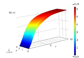
Figure 1: A three-dimensional plot for the solution $S(r,\theta)$ in the $CP^{1}$ model.

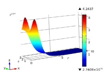
Figure 2: Energy density surface.

The energy density ${\cal E}^{CP^{1}}$ corresponding to the solution has two local maximums located on the $Z$-axis, Fig. 2. The energy is $18$ TeV, and the energy contribution from the first term in (17) is 51 % of the total energy in agreement with the analytic estimate based on Derrick’s theorem.

Existence of the exact numeric solution with the azimuthal magnetic flux in the Higgs subsector of the Weinberg-Salam model provides a strong indication to existence of a similar solution in the full theory where the Higgs boson is dressed by gauge $W,Z$ bosons. From ordinary considerations the energy of such a solution is expected to be of the same order. It is surprising, a careful numeric analysis presented below leads to energy estimate by one order less than $18$ TeV.

IV Magnetic solution with azimuthal magnetic flux

Let us consider possible magnetic solutions with a topological magnetic flux around the $Z$-axis in the pure bosonic sector of the Weinberg-Salam model. We apply a variational method to find field configurations which minimize the energy functional (16) with boundary conditions found from exact local solutions near the origin and space infinity. For numeric purpose we change the variable

$$Q(r,\theta)=\frac{1}{G(r,\theta)}-1,$$ (20)

and apply the following ansatz for static $SU(2)$ gauge potential in the temporal gauge $\vec{A}_{0}=0$

$$\vec{A}_{m} = A_{m}\hat{m}-\hat{m}\times\partial_{m}\hat{m}\,W(r,\theta).$$ (21)

With additional constraints $A_{r}=B_{r}=0$ one has eight trial functions $f,G,W,A_{\theta},A_{\varphi},B_{\theta},B_{\varphi},\rho$ dependent on two spherical coordinates $(r,\theta)$.

Note that, in ws1 we have studied a magnetic field configuration with azimuthal magnetic flux which minimizes the energy functional of Yang-Mills-Higgs theory. The energy estimate $4.3$ TeV for such a field configuration has been obtained in a special case when a constrained ansatz for the Higgs vector field $\hat{m}$ is applied, $f(r,\theta)=1$. All known solutions in the Yang-Mills-Higgs theory and in the Weinberg-Salam model (sphaleron, Cho-Maison monopole, monopole-antimonopole etc.) are studied within the Dashen-Hasslacher-Neveu (DHN) ansatz DHN ; manton83 which contains the same constraint $f(r,\theta)=1$. It is worth noting that the function $f(r,\theta)$ represents an independent degree of freedom of the Higgs boson and is supposed to be determined dynamically by equations of motion. So we conjecture that in general the field variable $f(r,\theta)$ should be a non-trivial function. We will consider two types of boundary conditions which correspond to two different local solutions near the origin $r=0$.

1 Type I boundary conditions

Full equations of motion of the Weinberg-Salam model represent highly non-linear partial differential equations for which the boundary value problem admits regular solutions not for arbitrary boundary conditions. To find proper boundary conditions one should solve equations of motion near boundaries and check consistency with finite energy conditions. We will find local solutions to the equations of motion of the Weinberg-Salam model in the vicinity of the origin $r=0$ and in the asymptotic infinity $r=\infty$ region. Substituting Taylor series expansions for the trial functions $f,G,W,A_{\theta},A_{\varphi},B_{\theta},B_{\varphi},\rho$ into all equations of motion one obtains the following local solution near the origin in lowest order approximation

$$f(r,\theta) = 1-2C_{1}r^{2}(5\cos^{2}\theta-1),$$

$$G(r,\theta) = \dfrac{6C_{1}C_{2}\kappa r^{3}}{\rho_{0}}(5\cos^{2}\theta-1),$$

$$W(r,\theta) = w_{0}+$$

$$\dfrac{(w_{0}-1)r^{2}}{88}(23C_{3}+11\rho_{0}+20C_{3}\cos(2\theta)),$$

$$A_{\theta}(r,\theta) = C_{2}\kappa r^{3}\sin\theta,$$

$$A_{\varphi}(r,\theta) = C_{3}r^{2}\sin^{2}\theta,$$

$$B_{\theta}(r,\theta) = C_{2}r^{3}\sin\theta,$$

$$B_{\varphi}(r,\theta) = -C_{3}r^{2}\sin^{2}\theta,$$

$$\rho(r,\theta) = \rho_{0}+r^{2}(C_{4}+\dfrac{6C_{2}\kappa}{\rho_{0}}+3C_{4}\cos(2\theta)),$$ (22)

where $C_{i},~{}w_{0},\rho_{0}$ are integration constants. We keep only those independent integration constants for which the solution satisfies the finite energy conditions and the symmetry under reflection $z\rightarrow-z$. A local finite energy solution in the asymptotic region at space infinity is given by the following expressions

$$f(r,\theta) = 1-2{\tilde{C}}_{1}\exp(-r),$$

$$G(r,\theta) = 1+\dfrac{{\tilde{C}}_{2}\kappa}{r^{2}}\exp(-\varkappa r),$$

$$W(r,\theta) = 1+\dfrac{{\tilde{C}}_{3}(1+r)}{r}\exp(-r),$$

$$A_{\theta}(r,\theta) = -{\tilde{C}}_{2}\kappa\exp(-\varkappa r)\sin\theta,$$

$$A_{\varphi}(r,\theta) = 1-\cos(2\theta)-\dfrac{{\tilde{C}}_{4}}{r}+{\tilde{C}}_{5}\kappa\exp(-\varkappa r)\sin^{2}\theta,$$

$$B_{\theta}(r,\theta) = -{\tilde{C}}_{2}\exp(-\varkappa r)\sin\theta,$$

$$B_{\varphi}(r,\theta) = \dfrac{{\tilde{C}}_{4}}{r}+{\tilde{C}}_{5}\exp(-\varkappa r)\sin^{2}\theta,$$

$$\rho(r,\theta) = 1+\dfrac{{\tilde{C}}_{6}}{r}\exp(-kr),$$

$$\varkappa^{2} \equiv 1+\frac{1}{\kappa},$$ (23)

where we keep only leading terms. Note that the solutions for azimuthal potentials $A_{\varphi},~{}B_{\varphi}$ include the term $\dfrac{{\tilde{C}}_{4}}{r}$ which provides long range behavior of the electromagnetic potential and corresponds to the dipole magnetic moment of the sphaleron solution. We will neglect this term in setting boundary conditions since we are interested in the magnetic solution with only one, azimuthal, non-vanishing magnetic field component. This can be reached by setting the constraints

$$A_{\varphi}+{\tilde{C}}_{\varphi}=0,~{}~{}~{}~{}~{}~{}~{}B_{\varphi}=0.$$ (24)

Notice, the above constraint has exactly the same structure as the gauge invariant quantity in (6). An additional variational analysis with a non-vanishing trial function for ${\tilde{C}}_{\varphi}$ shows that minimum of total energy is reached precisely when the constraint (24) is fulfilled.

The structure of the boundary conditions provides a minimal topological magnetic flux $2\pi$ of the azimuthal magnetic field through the half plane $P:\{y=0,~{}x\geq 0\}$

$$\Phi_{\varphi} = \int drd\theta{\cal F}_{r\theta}=\int drd\theta H_{r\theta}=2\pi.$$ (25)

In lowest order approximation we choose a simple radial dependence for the trial functions except for the function $A_{\theta}(r,\theta)$. The gauge field $A_{\theta}(r,\theta)$ provides a dominant contribution to the azimuthal magnetic field, so we keep two leading order terms in Fourier series expansion for that function to ensure a non-vanishing value of the first mode $A^{(1)}_{\theta}(r)$

$$A_{\theta}(r,\theta) = A^{(1)}_{\theta}(r)\sin\theta+A^{(2)}_{\theta}(r)\cos(2\theta).$$ (26)

With this setup we minimize the energy functional (16). The obtained variational profiles for the trial functions are shown in Fig. 3. The energy density in cylindrical coordinates has two maximums shown in Fig. 4, which correspond to two parallel circles coincided with the center lines of two tori in Cartesian coordinates, Fig. 5a. The total energy estimate is $1.36$ TeV. The surfaces of constant values for the energy density form tori or discs according to energy density values, Figs. 5a, 5b.

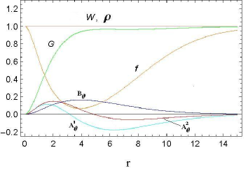
Figure 3: Trial functions: $f$-orange, $G$-green, $W$ - dashed, $A^{(1)}_{\theta}$ - cyan, $A_{\theta}^{(2)}$ - red, $B_{\theta}$ - blue, $\rho$ - pink

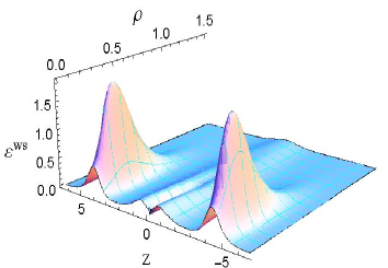
Figure 4: Energy density in cylindrical coordinates $(\rho,z)$.

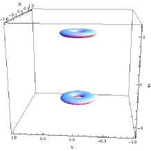
(a)  

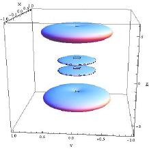
(b)  

Figure 5: Three-dimensional contour plots for the energy density surfaces in Cartesian coordinates $(X,Y,Z)$ for selected values: ${\cal E}^{WS}=1.5$, (a), and ${\cal E}^{WS}=0.157$, (b).

Low resolution leading to seemed irregularities in Fig. 5b (depicted by small squares) is caused by insufficient computer memory.

2 Type II boundary conditions

The local solution to the Weinberg-Salam equations near the origin $r=0$ (22) is not unique. Instead of Taylor series expansion for the trial functions one can apply perturbation theory to construct approximate solutions to the equations of motion. One can introduce a small parameter $\alpha$ which can be associated with the coupling constant $g$ or $g^{\prime}$ assuming they are small parameters. The perturbation theory with the parameter $\alpha$ can be consistently constructed since we use the dimensionless variables, so the couplings $g,~{}g^{\prime}$ are absorbed in dimensionless field variables as in (16). With this a new local solution near the origin can be obtained in the first order of the perturbation theory

$$f(r,\theta) = f_{0}+\alpha C_{1}(3-f_{0})r,$$

$$G(r,\theta) = G_{0}+\alpha C_{1}r,$$

$$W(r,\theta) = w_{0}+\alpha C_{2}r^{4}\cos^{2}\theta,$$

$$A_{\theta}(r,\theta) = \alpha\dfrac{C_{1}(3-f_{0})\rho_{0}^{2}}{12}r^{3}\sin\theta,$$

$$A_{\varphi}(r,\theta) = \alpha C_{3}r^{2}\sin^{2}\theta,$$

$$B_{\theta}(r,\theta) = -\alpha\dfrac{C_{1}(3-f_{0})\rho_{0}^{2}}{12}r^{3}\sin\theta,$$

$$B_{\varphi}(r,\theta) = \alpha C_{4}r^{2}\sin^{2}\theta,$$

$$\rho(r,\theta) = \rho_{0}+\alpha C_{5}r^{2}\big{(}1+3\cos(2\theta)\big{)},$$ (27)

where $C_{i},~{}f_{0},G_{0},w_{0},\rho_{0}$ are integration constants. Note that, due to the highly non-linear structure of the equations of motion to obtain the solution for $f,W$ in first order approximation one has to obtain solutions for other functions up to the second order of the perturbation theory. We present in the solution only terms of first order in $\alpha$ and leading terms in Taylor series expansion. We retain only those integration constants which provide the finite energy condition and symmetry under reflection $z\rightarrow-z$. In addition, we set $G_{0}=0$ whereas $f_{0},w_{0},\rho_{0}$ are treated as free variational parameters.

A local finite energy solution to Weinberg-Salam equations in the asymptotic region $r\simeq\infty$ is given by the same equations (23) as in the case of type I boundary conditions. As in the previous section we impose constraints (24) implying only azimuthal non-vanishing magnetic field component. The corresponding total magnetic flux around the $Z$-axis is $2\pi$. We keep two leading order terms in Fourier series expansion for the function $A_{\theta}$ as in (26).

The results of the variational procedure of minimizing the energy functional for the trial functions are presented in Fig. 6.

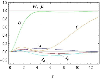
Figure 6: Trial functions: $f$-orange, $G$-green, $W$ - dashed, $A^{(1)}_{\theta}$ - cyan, $A_{\theta}^{(2)}$ - red, $B_{\theta}$ - blue, $\rho$ - pink

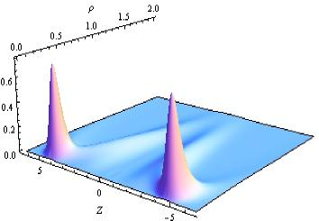
Figure 7: Energy density in cylindrical coordinates $(\rho,z)$.

Notice that the minimization procedure induces a zero value for the parameter $f_{0}$. We provide two types of boundary values for the function $f(r,\theta)$ since a solution with type I boundary conditions may exist even though it might be rather unstable. The energy density profile in cylindrical coordinates is plotted in Fig. 7. Qualitatively, the picture for the energy density is similar to the one in the case of a magnetic field configuration corresponding to type I boundary conditions: two maximums of the energy density are located along two circles with centers on the $Z$-axis. A total energy is $0.98$ TeV, which is much less than the energy value $18$ TeV of the magnetic field solution in the $CP^{1}$ model. Let us consider the electric current $\hat{J}_{n}$ which is responsible for the gauge invariant Abelian magnetic field ${\cal F}_{mn}$

$$\hat{J}_{n}=-\partial^{m}{\cal F}_{mn}.$$ (28)

In Fig. 8 we show that vector lines of the electric current $\hat{J}_{n}$ have a regular structure which has been checked at various scales in the interval $r=(0.01,30)$.

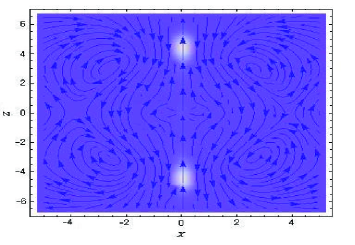
Figure 8: Vector stream plot for the electric current $\hat{J}_{n}$ in the plane $(X,Z)$ in Cartesian coordinates.

Certainly, the energy minimization procedure based on a restricted variational ansatz does not guarantee that local solutions near the origin and at infinity will match in the whole space. A rigorous approach should include Fourier series expansion for all fifteen variational functions within the most general axially-symmetric ansatz, or one should solve a complicated system of PDEs which has not been done so far except for cases of known solutions described by DHN ansatz.

In conclusion, we have demonstrated that interaction structure of the gauge and Higgs bosons implies existence of magnetic field configurations with energy upper bound near 1 TeV which is essentially less than energy of monopole like solutions in the Weinberg-Salam model. This would give rise to an attractive possibility for search of respective new bound states of $W,Z$ and Higgs bosons in concurrent experimental facilities.

- (1) M. Fairbairn, A. C. Kraan, D. A. Milstead, T. Sjostrand, P. Skands, T. Sloan, Phys. Rept. 438, pp. 1-63 (2007); arXiv: hep-ph/0611040.
- (2) K. A. Milton, Rept.Prog.Phys. 69, pp. 1637-1712 (2006); arXiv:hep-ex/0602040.
- (3) J. Pinfold, Rad. Meas. 44, 834 (2009); CERN Courier 52, No.7, 10 (2012).
- (4) B. Acharya et al, Int. J. Mod. Phys. A 29, 1430050 (2014).
- (5) P. A. M. Dirac, Phys. Rev. 74, 817 (1948).
- (6) T. T. Wu and C. N. Yang, Phys. Rev. D12, 3845 (1975).
- (7) Y. Nambu, Nucl. Phys. B130, 505 (1977).
- (8) Y. M. Cho and D. Maison, Phys. Lett. B391, 360 (1997).
- (9) D. G. Pak, P. M. Zhang and L. P. Zou, Int. J. Mod. Phys. A30, (2015) 1550164.
- (10) R. Dashen, B. Hasslacher and A. Neveu, Phys. Rev. D10 (1974) 4138.
- (11) N. S. Manton, Phys. Rev., D28, 2019 (1983).
- (12) F. R. Klinkhamer and N. S. Manton, Phys. Rev. D30, 2212, (1984).
- (13) M. Hindmarsh and M. James, Phys. Rev. D49, 6109 (1994).
- (14) Y. M. Cho, Phys. Rev. D21, 1080 (1980).
- (15) Y. S. Duan and Mo-Lin Ge, Sci. Sinica 11, 1072 (1979).
- (16) L. A. Ferreira, Wojtek J. Zakrzewski, JHEP 1309 (2013) 097; arXiv:1307.5856.
- (17) G. H. Derrick, J. Math. Phys. 5, 1252 (1964).