A Full Multigrid Method for Eigenvalue Problems

Abstract

In this paper, a full (nested) multigrid scheme is proposed to solve eigenvalue problems. The idea here is to use the multilevel correction method to transform the solution of eigenvalue problem to a series of solutions of the corresponding boundary value problems and eigenvalue problems defined on the coarsest finite element space. The boundary value problems which are define on a sequence of multilevel finite element space can be solved by some multigrid iteration steps. Besides the multigrid iteration, all other efficient iteration methods for solving boundary value problems can serve as linear problem solver. The computational work of this new scheme can reach optimal order the same as solving the corresponding source problem. Therefore, this type of iteration scheme improves the efficiency of eigenvalue problem solving.

Keywords. Eigenvalue problem, full multigrid method, multilevel correction, finite element method.

AMS subject classifications. 65N30, 65N25, 65L15, 65B99.

1 Introduction

It is well known there have existed many efficient algorithms, such as multigrid method and many other precondition techniques [8, 17, 21], for solving boundary value problems. The error bounds of the approximate solution obtained from these efficient numerical algorithms are comparable to the theoretical bounds determined by the finite element discretization. But the amount of computational work involved is only proportional to the number of unknowns in the discretized equations. For more details of the multigrid and multilevel methods, please refer to [4, 5, 6, 7, 8, 11, 12, 15, 16, 17, 21, 22] and the references cited therein.

But there is no many efficient numerical methods for solving eigenvalue problems with optimal complexity. Solving large scale eigenvalue problems is one of fundamental problems in modern science and engineering society. However, it is always a very difficult task to solve high-dimensional eigenvalue problems which come from physical and chemistry sciences. Recently, a type of multilevel correction method is proposed for solving eigenvalue problems in [13, 19, 20]. In this multilevel correction scheme, the solution of eigenvalue problem on the final level mesh can be reduced to a series of solutions of boundary value problems on the multilevel meshes and a series of solutions of the eigenvalue problem on the coarsest mesh. The multilevel correction method gives a way to construct the multigrid method for eigenvalue problems [19, 20].

The aim of this paper is to present a full multigrid method for solving eigenvalue problems based on the combination of the multilevel correction method [19, 20] and the multigrid iteration for boundary value problems. Comparing with the method in [13, 19, 20], the difference is that we do not solve the linear boundary value problem exactly in each correction step with the multigrid method. We only get an approximate solution with some multigrid iteration steps. In this new version of multigrid method, solving eigenvalue problem will not be much more difficult than the multigrid scheme for the corresponding boundary value problems. It is worth to noting that besides the multigrid method here, other types of numerical algorithms such as BPX multilevel preconditioners [21], algebraic multigrid method and domain decomposition preconditioners (cf. [8, 18]) can also act as the linear algebraic solvers for boundary value problems.

An outline of the paper goes as follows. In Section 2, we introduce the finite element method for eigenvalue problem and the corresponding basic error estimates. A type of full multigrid algorithm for solving eigenvalue problem by finite element method is given in Section 3. Two numerical examples are presented to validate our theoretical analysis in section 4. Some concluding remarks are given in the last section.

2 Finite element method for eigenvalue problem

This section is devoted to introducing some notation and the finite element method for eigenvalue problem. In this paper, we shall use the standard notation for Sobolev spaces $W^{s,p}(\Omega)$ and their associated norms and semi-norms (cf. [1]). For $p=2$, we denote $H^{s}(\Omega)=W^{s,2}(\Omega)$ and $H_{0}^{1}(\Omega)=\{v\in H^{1}(\Omega):\ v|_{\partial\Omega}=0\}$, where $v|_{\Omega}=0$ is in the sense of trace, $\|\cdot\|_{s,\Omega}=\|\cdot\|_{s,2,\Omega}$. The letter $C$ (with or without subscripts) denotes a generic positive constant which may be different at its different occurrences through the paper.

For simplicity, we consider the following model problem to illustrate the main idea: Find $(\lambda,u)$ such that

$$\left\{\begin{array}[]{rcl}-\nabla\cdot(\mathcal{A}\nabla u)+\phi u&=&\lambda u,\quad{\rm in}\ \Omega,\\ u&=&0,\ \ \quad{\rm on}\ \partial\Omega,\end{array}\right.$$ (2.1)

where $\mathcal{A}$ is a symmetric and positive definite matrix with suitable regularity, $\phi$ is a nonnegative function, $\Omega\subset\mathcal{R}^{d}$ $(d=2,3)$ is a bounded domain with Lipschitz boundary $\partial\Omega$ and $\nabla$, $\nabla\cdot$ denote the gradient, divergence operators, respectively.

In order to use the finite element method to solve the eigenvalue problem (2.1), we need to define the corresponding variational form as follows: Find $(\lambda,u)\in\mathcal{R}\times V$ such that $b(u,u)=1$ and

$$a(u,v) = \lambda b(u,v),\quad\forall v\in V,$$ (2.2)

where $V:=H_{0}^{1}(\Omega)$ and

$$a(u,v)=\int_{\Omega}\big{(}\nabla u\cdot\mathcal{A}\nabla v+\phi uv\big{)}d\Omega,\ \ \ \ \ \ b(u,v)=\int_{\Omega}uvd\Omega.$$ (2.3)

The norms $\|\cdot\|_{a}$ and $\|\cdot\|_{b}$ are defined by

$$\|v\|_{a}=a(v,v)^{1/2}\ \ \ \ \ {\rm and}\ \ \ \ \ \|v\|_{b}=b(v,v)^{1/2}.$$

It is well known that the eigenvalue problem (2.2) has an eigenvalue sequence $\{\lambda_{j}\}$ (cf. [3, 9]):

$$0<\lambda_{1}\leq\lambda_{2}\leq\cdots\leq\lambda_{k}\leq\cdots,\ \ \ \lim_{k\rightarrow\infty}\lambda_{k}=\infty,$$

and associated eigenfunctions

$$u_{1},u_{2},\cdots,u_{k},\cdots,$$

where $b(u_{i},u_{j})=\delta_{ij}$ ($\delta_{ij}$ denotes the Kronecker function). In the sequence $\{\lambda_{j}\}$, the $\lambda_{j}$ are repeated according to their geometric multiplicity.

Now, let us define the finite element approximations of the problem (2.2). First we generate a shape-regular decomposition of the computing domain $\Omega\subset\mathcal{R}^{d}\ (d=2,3)$ into triangles or rectangles for $d=2$ (tetrahedrons or hexahedrons for $d=3$) (cf. [8, 10]). The diameter of a cell $K\in\mathcal{T}_{h}$ is denoted by $h_{K}$ and the mesh size $h$ describes the maximum diameter of all cells $K\in\mathcal{T}_{h}$. Based on the mesh $\mathcal{T}_{h}$, we can construct a finite element space denoted by $V_{h}\subset V$. For simplicity, we set $V_{h}$ as the linear finite element space which is defined as follows

$$V_{h}=\big{\{}v_{h}\in C(\Omega)\ \big{|}\ v_{h}|_{K}\in\mathcal{P}_{1},\ \ \forall K\in\mathcal{T}_{h}\big{\}},$$ (2.4)

where $\mathcal{P}_{1}$ denotes the linear function space.

The standard finite element scheme for eigenvalue problem (2.2) is: Find $(\bar{\lambda}_{h},\bar{u}_{h})\in\mathcal{R}\times V_{h}$ such that $b(\bar{u}_{h},\bar{u}_{h})=1$ and

$$a(\bar{u}_{h},v_{h}) = \bar{\lambda}_{h}b(\bar{u}_{h},v_{h}),\quad\ \ \ \forall v_{h}\in V_{h}.$$ (2.5)

From [2, 3, 9], the discrete eigenvalue problem (2.5) has eigenvalues:

$$0<\bar{\lambda}_{1,h}\leq\bar{\lambda}_{2,h}\leq\cdots\leq\bar{\lambda}_{k,h}\leq\cdots\leq\bar{\lambda}_{N_{h},h},$$

and corresponding eigenfunctions

$$\bar{u}_{1,h},\bar{u}_{2,h},\cdots,\bar{u}_{k,h},\cdots,\bar{u}_{N_{h},h},$$

where $b(\bar{u}_{i,h},\bar{u}_{j,h})=\delta_{ij},1\leq i,j\leq N_{h}$ ($N_{h}$ is the dimension of the finite element space $V_{h}$).

Let $M(\lambda_{i})$ denote the eigenspace corresponding to the eigenvalue $\lambda_{i}$ which is defined by

$$M(\lambda_{i}) = \big{\{}w\in H_{0}^{1}(\Omega):w\ {\rm is\ an\ eigenvalue\ of\ (\ref{weak_eigenvalue_problem})}$$ (2.6)

$$\ \ \ \ \ \ \ \ \ \ \ \ \ {\rm corresponding\ to}\ \lambda_{i}\ {\rm and}\ b(w,w)=1\big{\}},$$

and define

$$\delta_{h}(\lambda_{i})=\sup_{w\in M(\lambda_{i})}\inf_{v_{h}\in V_{h}}\|w-v_{h}\|_{a}.$$ (2.7)

Let us define the following quantity:

$$\eta_{a}(h) = \sup_{f\in L^{2}(\Omega),\|f\|_{b}=1}\inf_{v_{h}\in V_{h}}\|Tf-v_{h}\|_{a},$$ (2.8)

where $T:L^{2}(\Omega)\rightarrow V$ is defined as

$$a(Tf,v)=b(f,v),\ \ \ \ \ \forall f\in L^{2}(\Omega)\ \ \ {\rm and}\ \ \ \forall v\in V.$$ (2.9)

Then the error estimates for the eigenpair approximations by the finite element method can be described as follows.

Lemma 2.1.

([2, Lemma 3.6, Theorem 4.4] and [9]) For any eigenpair approximation $(\bar{\lambda}_{i,h},\bar{u}_{i,h})$ $(i=1,2,\cdots,N_{h})$ of (2.5), there exists an exact eigenpair $(\lambda_{i},u_{i})$ of (2.2) such that $b(u_{i},u_{i})=1$ and

$$\|u_{i}-\bar{u}_{i,h}\|_{a} \leq \big{(}1+C_{i}\eta_{a}(h)\big{)}\delta_{h}(\lambda_{i}),$$ (2.10)

$$\|u_{i}-\bar{u}_{i,h}\|_{b} \leq C_{i}\eta_{a}(h)\|u_{i}-u_{i,h}\|_{a},$$ (2.11)

$$|\lambda_{i}-\bar{\lambda}_{i,h}| \leq C_{i}\|u_{i}-\bar{u}_{i,h}\|_{a}^{2}.$$ (2.12)

Here and hereafter $C_{i}$ is some constant depending on $i$ but independent of the mesh size $h$.

3 Full multigrid algorithm for eigenvalue problem

Recently, a multilevel correction scheme is introduced in [13, 19, 20] for solving eigenvalue problems. Based on the idea of multilevel correction scheme, we propose a type of full multigrid method for eigenvalue problems here. The main idea in this method is to approximate the underlying boundary value problems on each level by some multigrid smoothing iteration steps. In order to describe the full multigrid method, we first introduce the sequence of finite element spaces. We generate a coarse mesh $\mathcal{T}_{H}$ with the mesh size $H$ and the coarse linear finite element space $V_{H}$ is defined on the mesh $\mathcal{T}_{H}$. Then we define a sequence of triangulations $\mathcal{T}_{h_{k}}$ of $\Omega\subset\mathcal{R}^{d}$ determined as follows. Suppose $\mathcal{T}_{h_{1}}$ (produced from $\mathcal{T}_{H}$ by regular refinements) is given and let $\mathcal{T}_{h_{k}}$ be obtained from $\mathcal{T}_{h_{k-1}}$ via one regular refinement step (produce $\beta^{d}$ subelements) such that

$$h_{k}=\frac{1}{\beta}h_{k-1},\ \ \ \ k=2,\cdots,n,$$ (3.1)

where the positive number $\beta$ denotes the refinement index and larger than $1$ (always equals $2$). Based on this sequence of meshes, we construct the corresponding nested linear finite element spaces such that

$$V_{H}\subseteq V_{h_{1}}\subset V_{h_{2}}\subset\cdots\subset V_{h_{n}}.$$ (3.2)

The sequence of finite element spaces $V_{h_{1}}\subset V_{h_{2}}\subset\cdots\subset V_{h_{n}}$ and the finite element space $V_{H}$ have the following relations of approximation accuracy

$$\eta_{a}(H)\gtrsim\delta_{h_{1}}(\lambda_{i}),\ \ \ \ \delta_{h_{k}}(\lambda_{i})=\frac{1}{\beta}\delta_{h_{k-1}}(\lambda_{i}),\ \ \ k=2,\cdots,n.$$ (3.3)

3.1 One correction step

In order to design the full multigrid method, we introduce an one correction step in this subsection.

Assume we have obtained an eigenpair approximation $(\lambda_{\ell,h_{k}},u_{\ell,h_{k}})\in\mathcal{R}\times V_{h_{k}}$. Now we introduce a type of iteration step to improve the accuracy of the current eigenpair approximation $(\lambda_{\ell,h_{k}},u_{\ell,h_{k}})$.

Algorithm 3.1.

One Correction Step

1. Define the following auxiliary source problem: Find $\widehat{u}_{\ell+1,h_{k}}\in V_{h_{k}}$ such that

   $$a(\widehat{u}_{\ell+1,h_{k}},v_{h_{k}}) = \lambda_{\ell,h_{k}}b(u_{\ell,h_{k}},v_{h_{k}}),\ \ \ \forall v_{h_{k}}\in V_{h_{k}}.$$ (3.4)

   Perform $m$ multigrid iteration steps with the initial value $u_{\ell,h_{k}}$ to obtain a new eigenfunction approximation $\widetilde{u}_{\ell+1,h_{k}}\in V_{h_{k}}$ by

   $$\widetilde{u}_{\ell+1,h_{k}}=MG(V_{h_{k}},\lambda_{\ell,h_{k}}u_{\ell,h_{k}},u_{\ell,h_{k}},m),$$ (3.5)

   where $V_{h_{k}}$ denotes the working space for the multigrid iteration, $\lambda_{\ell,h_{k}}u_{\ell,h_{k}}$ is the right hand side term of the linear equation, $u_{\ell,h_{k}}$ denotes the initial guess and $m$ is the number of multigrid iteration times.

2. Define a new finite element space $V_{H,h_{k}}=V_{H}+{\rm span}\{\widetilde{u}_{\ell+1,h_{k}}\}$ and solve the following eigenvalue problem: Find $(\lambda_{\ell+1,h_{k}},u_{\ell+1,h_{k}})\in\mathcal{R}\times V_{H,h_{k}}$ such that $b(u_{\ell+1,h_{k}},u_{\ell+1,h_{k}})=1$ and

   $$a(u_{\ell+1,h_{k}},v_{H,h_{k}}) = \lambda_{\ell+1,h_{k}}b(u_{\ell+1,h_{k}},v_{H,h_{k}}),\ \ \ \forall v_{H,h_{k}}\in V_{H,h_{k}}.$$ (3.6)

In order to simplify the notation and summarize the above two steps, we define

$$(\lambda_{\ell+1,h_{k}},u_{\ell+1,h_{k}})=EigenMG(V_{H},\lambda_{\ell,h_{k}},u_{\ell,h_{k}},V_{h_{k}},m).$$

Theorem 3.1.

Assume the multigrid iteration $\widetilde{u}_{\ell+1,h_{k}}=MG(V_{h_{k}},\lambda_{\ell,h_{k}}u_{\ell,h_{k}},u_{\ell,h_{k}},m)$ has the following error reduction rate

$$\|\widehat{u}_{\ell+1,h_{k}}-\widetilde{u}_{\ell+1,h_{k}}\|_{a}\leq\theta\|\widehat{u}_{\ell+1,h_{k}}-u_{\ell,h_{k}}\|_{a},$$ (3.7)

and $(\lambda_{\ell,h_{k}},u_{\ell,h_{k}})$ has the following properties

$$\|\bar{u}_{h_{k}}-u_{\ell,h_{k}}\|_{b} \leq C_{i}\eta_{a}(H)\|\bar{u}_{h_{k}}-u_{\ell,h_{k}}\|_{a},$$ (3.8)

$$|\bar{\lambda}_{h_{k}}-\lambda_{\ell,h_{k}}| \leq C_{i}\|\bar{u}_{h_{k}}-u_{\ell,h_{k}}\|_{a}^{2}.$$ (3.9)

After performing the one correction step defined in Algorithm 3.1, the resultant eigenpair approximation $(\lambda_{\ell+1,h_{k}},u_{\ell+1,h_{k}})\in\mathcal{R}\times V_{h_{k}}$ has the following error estimates

$$\|\bar{u}_{h_{k}}-u_{\ell+1,h_{k}}\|_{a} \leq \gamma\|\bar{u}_{h_{k}}-u_{\ell,h_{k}}\|_{a},$$ (3.10)

$$\|\bar{u}_{h_{k}}-u_{\ell+1,h_{k}}\|_{b} \leq C_{i}\eta_{a}(H)\|\bar{u}_{h_{k}}-u_{\ell+1,h_{k}}\|_{a},$$ (3.11)

$$|\bar{\lambda}_{h_{k}}-\lambda_{\ell+1,h_{k}}| \leq C_{i}\|\bar{u}_{h_{k}}-u_{\ell+1,h_{k}}\|_{a}^{2}.$$ (3.12)

where

$$\gamma=\theta+(1+2\theta)C_{i}\eta_{a}(H)+(1+\theta)C_{i}^{2}\eta_{a}^{2}(H).$$ (3.13)

Proof.

From (2.5) and (3.4), we have

$$a(\bar{u}_{h_{k}}-\widehat{u}_{\ell+1,h_{k}},v_{h_{k}})=b(\bar{\lambda}_{h_{k}}\bar{u}_{h_{k}}-\lambda_{\ell,h_{k}}u_{\ell,h_{k}},v_{h_{k}}),\ \ \ \ \forall v_{h_{k}}\in V_{h_{k}}.$$ (3.14)

It leads to the following estimates

$$\|\bar{u}_{h_{k}}-\widehat{u}_{\ell+1,h_{k}}\|_{a} \leq \|\bar{\lambda}_{h_{k}}\bar{u}_{h_{k}}-\lambda_{\ell,h_{k}}u_{\ell,h_{k}}\|_{b}$$ (3.15)

$$\leq |\bar{\lambda}_{h_{k}}-\lambda_{\ell,h_{k}}|+\|\bar{u}_{h_{k}}-u_{\ell,h_{k}}\|_{b}$$

$$\leq C_{i}\eta_{a}(H)\|\bar{u}_{h_{k}}-u_{\ell,h_{k}}\|_{a}.$$

Combining (3.7) and (3.15) leads to the following linear solving error estimate for $\widetilde{u}_{\ell+1,h_{k}}$

$$\|\widehat{u}_{\ell+1,h_{k}}-\widetilde{u}_{\ell+1,h_{k}}\|_{a} \leq \theta\|\widehat{u}_{\ell+1,h_{k}}-u_{\ell,h_{k}}\|_{a}$$ (3.16)

$$\leq \theta\big{(}\|\widehat{u}_{\ell+1,h_{k}}-\bar{u}_{h_{k}}\|_{a}+\|\bar{u}_{h_{k}}-u_{\ell,h_{k}}\|_{a}\big{)}$$

$$\leq \theta\big{(}1+C_{i}\eta_{a}(H)\big{)}\|\bar{u}_{h_{k}}-u_{\ell,h_{k}}\|_{a}.$$

Then from (3.15) and (3.16), we have the following inequalities

$$\|\bar{u}_{h_{k}}-\widetilde{u}_{\ell+1,h_{k}}\|_{a} \leq \|\bar{u}_{h_{k}}-\widehat{u}_{\ell+1,h_{k}}\|_{a}+\|\widehat{u}_{\ell+1,h_{k}}-\widetilde{u}_{\ell+1,h_{k}}\|_{a}$$ (3.17)

$$\leq \big{(}\theta+(1+\theta)C_{i}\eta_{a}(H)\big{)}\|\bar{u}_{h_{k}}-u_{\ell,h_{k}}\|_{a}.$$

The eigenvalue problem (3.6) can be regarded as a finite dimensional subspace approximation of the eigenvalue problem (2.5). Similarly to Lemma 2.1 (see [2, Theorem 4.4]), from the second step in Algorithm 3.1 and (3.17), the following estimates hold

$$\|\bar{u}_{h_{k}}-u_{\ell+1,h_{k}}\|_{a} \leq \big{(}1+C_{i}\widetilde{\eta}_{a}(H)\big{)}\inf_{v_{H,h_{k}}\in V_{H,h_{k}}}\|\bar{u}_{h_{k}}-v_{H,h_{k}}\|_{a}$$ (3.18)

$$\leq \big{(}1+C_{i}\eta_{a}(H)\big{)}\|\bar{u}_{h_{k}}-\widetilde{u}_{\ell+1,h_{k}}\|_{a}$$

$$\leq \gamma\|\bar{u}_{h_{k}}-u_{\ell,h_{k}}\|_{a}$$

and

$$\|\bar{u}_{h_{k}}-u_{\ell+1,h_{k}}\|_{b} \leq C_{i}\widetilde{\eta}_{a}(H)\|\bar{u}_{h_{k}}-u_{\ell+1,h_{k}}\|_{a}$$ (3.19)

$$\leq C_{i}\eta_{a}(H)\|\bar{u}_{h_{k}}-u_{\ell+1,h_{k}}\|_{a},$$

$$|\bar{\lambda}_{h_{k}}-\lambda_{\ell+1,h_{k}}| \leq C_{i}\|\bar{u}_{h_{k}}-u_{\ell+1,h_{k}}\|_{a}^{2},$$ (3.20)

where

$$\widetilde{\eta}_{a}(H) = \sup_{f\in V,\|f\|_{0}=1}\inf_{v\in V_{H,h_{k}}}\|Tf-v\|_{a}\leq\eta_{a}(H).$$ (3.21)

Then we obtained the desired results (3.10)-(3.12) and complete the proof. ∎

3.2 Full multigrid method for eigenvalue problem

In this subsection, we introduce a full multigrid scheme based on the One Correction Step defined in Algorithm 3.1. This type of full multigrid method can obtain the optimal error estimate with the optimal computational work.

Since the multigrid method for the boundary value problem has the uniform error reduction rate, we can choose suitable $m$ such that $\theta<1$ in (3.7). From (3.13), we have $\gamma<1$ if $H$ is small enough. From this observation, we can build the following full multigrid method for solving eigenvalue problems.

Algorithm 3.2.

Full Multigrid Scheme

1. Solve the following eigenvalue problem in $V_{h_{1}}$: Find $(\lambda_{h_{1}},u_{h_{1}})\in\mathcal{R}\times V_{h_{1}}$ such that

   $$a(u_{h_{1}},v_{h_{1}})=\lambda_{h_{1}}b(u_{h_{1}},v_{h_{1}}),\quad\forall v_{h_{1}}\in V_{h_{1}}.$$

   Solve this eigenvalue problem to get an eigenpair approximation $(\lambda_{h_{1}},u_{h_{1}})\in\mathcal{R}\times V_{h_{1}}$.

2. For $k=2,\cdots,n$, do the following iteration

   • Set $u_{0,h_{k}}=u_{h_{k-1}}$.

   • Do the following multigrid iteration

     $$(\lambda_{\ell+1,h_{k}},u_{\ell+1,h_{k}})=EigenMG(V_{H},\lambda_{\ell,h_{k}},u_{\ell,h_{k}},V_{h_{k}},m),\ \ \ \ {\rm for}\ \ell=0,\cdots,p-1.$$

   • set $\lambda_{h_{k}}=\lambda_{p,h_{k}}$ and $u_{h_{k}}=u_{p,h_{k}}$.

   end Do

Finally, we obtain an eigenpair approximation $(\lambda_{h_{n}},u_{h_{n}})\in\mathcal{R}\times V_{h_{n}}$.

Theorem 3.2.

After implementing Algorithm 3.2, the resultant eigenpair approximation $(\lambda_{h_{n}},u_{h_{n}})$ has the following error estimate

$$\|\bar{u}_{h_{n}}-u_{h_{n}}\|_{a} \leq C\frac{\gamma^{p}}{1-\beta\gamma^{p}}\delta_{h_{n}}(\lambda),$$ (3.22)

$$|\bar{\lambda}_{h_{n}}-\lambda_{h_{n}}| \leq C\delta_{h_{n}}^{2}(\lambda),$$ (3.23)

under the condition $\beta\gamma^{p}<1$.

Proof.

Define $e_{k}:=\bar{u}_{h_{k}}-u_{h_{k}}$. Then from step 1 in Algorithm 3.2, it is obvious $e_{1}=0$. For $k=2,\cdots,n$, we have

$$\|e_{k}\|_{a} \leq \gamma^{p}\|\bar{u}_{h_{k}}-u_{h_{k-1}}\|_{a}$$ (3.24)

$$\leq \gamma^{p}\big{(}\|\bar{u}_{h_{k}}-\bar{u}_{h_{k-1}}\|_{a}+\|\bar{u}_{h_{k-1}}-u_{h_{k-1}}\|_{a}\big{)}$$

$$\leq \gamma^{p}\big{(}C\delta_{h_{k}}(\lambda)+\|e_{k-1}\|_{a}\big{)}.$$

By iterating inequality (3.24) and $\beta\gamma^{p}<1$, the following inequalities hold

$$\|e_{n}\|_{a} \leq C\gamma^{p}\delta_{h_{n}}(\lambda)+C\gamma^{2p}\delta_{h_{n-1}}(\lambda)+\cdots+C\gamma^{(n-1)p}\delta_{h_{2}}(\lambda)$$ (3.25)

$$\leq C\sum_{k=2}^{n}\gamma^{(n-k+1)p}\delta_{h_{\ell}}(\lambda)=C\left(\sum_{k=2}^{n}\big{(}\beta\gamma^{p}\big{)}^{n-k}\right)\gamma^{p}\delta_{h_{n}}(\lambda)$$

$$\leq C\frac{\gamma^{p}}{1-\beta\gamma^{p}}\delta_{h_{n}}(\lambda).$$

For such choice of $p$, we arrive the desired result (3.22) and (3.23) can be obtained by (2.12) and (3.22). ∎

Remark 3.1.

The good convergence rate of the multigrid method for boundary value problems leads to that we do not need to choose large $m$ and $p$ [8, 12, 17, 21].

Now we turn our attention to the estimate of computational work for Full Multigrid Scheme 3.2. We will show that Algorithm 3.2 makes solving eigenvalue problem need almost the same work as solving the corresponding boundary value problem.

First, we define the dimension of each level finite element space as $N_{k}:={\rm dim}V_{h_{k}}$. Then we have

$$N_{k}=\Big{(}\frac{1}{\beta}\Big{)}^{d(n-k)}N_{n},\ \ \ k=1,2,\cdots,n.$$ (3.26)

Theorem 3.3.

Assume the eigenvalue problem solved in the coarse spaces $V_{H}$ and $V_{h_{1}}$ need work $\mathcal{O}(M_{H})$ and $\mathcal{O}(M_{h_{1}})$, respectively, and the work of the multigrid solver $MG(V_{h_{k}},\lambda_{\ell,h_{k}}u_{\ell,h_{k}},u_{\ell,h_{k}},m)$ in each level space $V_{h_{k}}$ is $\mathcal{O}(N_{k})$ for $k=2,3,\cdots,n$. Then the work involved in the Full Multigrid Scheme 3.2 is $\mathcal{O}(N_{n}+M_{H}\log(N_{n})+M_{h_{1}})$. Furthermore, the complexity will be $\mathcal{O}(N_{n})$ provided $M_{H}\ll N_{k}$ and $M_{h_{1}}\leq N_{k}$.

Proof.

Let $W_{k}$ denote the work in the correction step in the $k$-th finite element space $V_{h_{k}}$. Then with the correction definition in Algorithm 3.1, we have

$$W_{k} = \mathcal{O}(N_{k}+M_{H}),\ \ \ \ \ k=2,\cdots,n.$$ (3.27)

Iterating (3.27) and using the fact (3.26), we obtain

$${\rm Total\ work} = \sum_{k=1}^{n}W_{k}=\mathcal{O}\Big{(}M_{h_{1}}+\sum_{k=2}^{n}\big{(}N_{k}+M_{H}\big{)}\Big{)}$$

$$= \mathcal{O}\Big{(}M_{h_{1}}+(n-1)M_{H}+\sum_{k=2}^{n}\big{(}\frac{1}{\beta}\big{)}^{d(n-k)}N_{n}\Big{)}$$

$$= \mathcal{O}(N_{n}+M_{H}\log N_{n}+M_{h_{1}}).$$

This is the desired result $\mathcal{O}(N_{n}+M_{H}\log N_{n}+M_{h_{1}})$ and the one $\mathcal{O}(N_{n})$ can be obtained by the conditions $M_{H}\ll N_{n}$ and $M_{h_{1}}\leq N_{n}$. ∎

4 Numerical results

In this section, two numerical examples are presented to illustrate the efficiency of the full multigrid scheme proposed in this paper.

4.1 Model eigenvalue problem

Here we give the numerical results of the full multigrid scheme for the model eigenvalue problem: Find $(\lambda,u)$ such that

$$\left\{\begin{array}[]{rcl}-\Delta u&=&\lambda u,\quad{\rm in}\ \Omega,\\ u&=&0,\quad\ \ {\rm on}\ \partial\Omega,\\ \int_{\Omega}u^{2}d\Omega&=&1,\end{array}\right.$$ (4.1)

where $\Omega=(0,1)\times(0,1)$.

The sequence of finite element spaces are constructed by using linear element on the series of meshes which are produced by regular refinement with $\beta=2$ (connecting the midpoints of each edge). In this example, we use two meshes which are generated by Delaunay method as the initial mesh $\mathcal{T}_{h_{1}}$ and set $\mathcal{T}_{H}=\mathcal{T}_{h_{1}}$ to investigate the convergence behaviors. Figure 1 shows the corresponding initial meshes: one is coarse and the other is fine.

Algorithm 3.2 is applied to solve the eigenvalue problem. In this subsection, we choose $m=2$ and $2$ conjugate gradient smoothing steps for the presmoothing and postsmoothing in each multigrid iteration step in Algorithm 3.1. In each level of the full multigrid scheme defined in Algorithm 3.2, we only do $2$ multigrid iteration steps ($p=2$) defined in Algorithm 3.1. For comparison, we also solve the eigenvalue problem by the direct method.

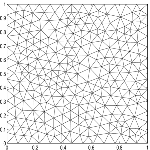
Figure 1: The coarse and fine initial meshes for the unit square

Figure 2 gives the corresponding numerical results for the first eigenvalue $\lambda_{1}=2\pi^{2}$ and the corresponding eigenfunction on the two initial meshes illustrated in Figure 1.

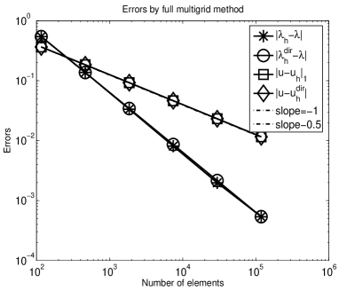
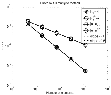
Figure 2: The errors of the full multigrid algorithm for the first six eigenvalues on the unit square, where $u_{h}$ and $\lambda_{h}$ denote the eigenfunction and eigenvalue approximations by Algorithm 3.2, and $u_{h}^{\rm dir}$ and $\lambda_{h}^{\rm dir}$ denote the eigenfunction and eigenvalue approximation by direct eigenvalue solving (The left figure corresponds to the left mesh in Figure 1 and the right figure corresponds to the right mesh in Figure 1)

From Figure 2, we find the full multigrid scheme can obtain the optimal error estimates as same as the direct eigenvalue problem solving for the eigenvalue and the corresponding eigenfunction approximations.

We also check the convergence behavior for multi eigenvalue approximations with Algorithm 3.2. Here the first six eigenvalues $\lambda=2\pi^{2},5\pi^{2},5\pi^{2},8\pi^{2},$ $10\pi^{2},10\pi^{2}$ are investigated. We adopt the meshes in Figure 1 as the initial meshes and the corresponding numerical results are shown in Figure 3 which also exhibits the optimal convergence of the full multigrid scheme.

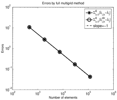
Figure 3: The errors of the full multigrid algorithm for the first six eigenvalues on the unit square, $\lambda_{h}$ denotes the eigenvalue approximation by Algorithm 3.2, $\lambda_{h}^{\rm dir}$ denotes the eigenvalue approximation by direct eigenvalue solving (The left figure corresponds to the left mesh in Figure 1 and the right figure corresponds to the right mesh in Figure 1)

4.2 More general eigenvalue problem

Here we give numerical results of the full multigrid method for solving a more general eigenvalue problem on the unit square domain $\Omega=(0,1)\times(0,1)$: Find $(\lambda,u)$ such that

$$\left\{\begin{array}[]{rcl}-\nabla\cdot\mathcal{A}\nabla u+\phi u&=&\lambda\rho u,\quad{\rm in}\ \Omega,\\ u&=&0,\quad\ \ \ {\rm on}\ \partial\Omega,\\ \int_{\Omega}\rho u^{2}d\Omega&=&1,\end{array}\right.$$ (4.2)

where

$$\mathcal{A}=\left(\begin{array}[]{cc}$$1+(x_{1}-\frac{1}{2})^{2}$$&$$(x_{1}-\frac{1}{2})(x_{2}-\frac{1}{2})$$\\ $$(x_{1}-\frac{1}{2})(x_{2}-\frac{1}{2})$$&$$1+(x_{2}-\frac{1}{2})^{2}$$\end{array}\right),$$

$\phi=e^{(x_{1}-\frac{1}{2})(x_{2}-\frac{1}{2})}$ and $\rho=1+(x_{1}-\frac{1}{2})(x_{2}-\frac{1}{2})$.

In this example, we also use two coarse meshes which are shown in Figure 1 as the initial meshes to investigate the convergence behaviors. Since the exact solution is not known, we choose an adequately accurate eigenvalue approximations with the extrapolation method (see, e.g., [14]) as the exact eigenvalues to measure errors. Figure 4 gives the corresponding numerical results for the first six eigenvalue approximations. In this example, we also choose $m=2$, $p=2$ and $2$ conjugate gradient smoothing step in the presmoothing and postsmoothing procedure. Here we also compare the numerical results with the direct algorithm. The corresponding results are shown in Figure 4 which also exhibits the optimality of the error and complexity for Algorithm 3.2.

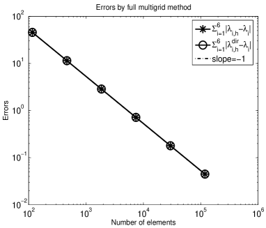
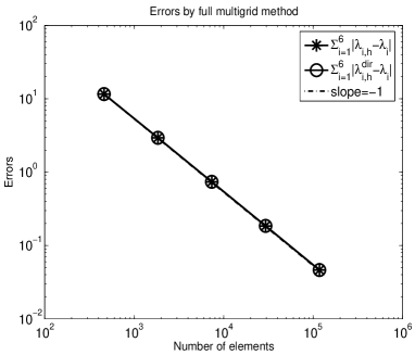
Figure 4: The errors of the full multigrid algorithm for the first six eigenvalues on the unit square, $\lambda_{h}$ denotes the eigenvalue approximation by Algorithm 3.2, $\lambda_{h}^{\rm dir}$ denotes the eigenvalue approximation by direct eigenvalue solving (The left figure corresponds to the left mesh in Figure 1 and the right figure corresponds to the right mesh in Figure 1)

5 Concluding remarks

In this paper, we give a full multigrid scheme to solve eigenvalue problems. The idea here is to use the multilevel correction method to transform the solution of the eigenvalue problem to a series of solutions of the corresponding boundary value problems, which can be solved by some multigrid iteration steps, and solutions of eigenvalue problems defined on the coarsest finite element space.

We can replace the multigrid iteration by other types of efficient iteration schemes such as algebraic multigrid method, the type of preconditioned schemes based on the subspace decomposition and subspace corrections (see, e.g., [8, 21]), and the domain decomposition method (see, e.g., [18, 23]). The ideas can be extended to other types of linear and nonlinear eigenvalue problems and other types problems. These will be investigated in our future work.

References

• [1] R. A. Adams, Sobolev Spaces, Academic Press, New York, 1975.
• [2] I. BabuΕ‘ka and J. E. Osborn, Finite element-Galerkin approximation of the eigenvalues and eigenvectors of selfadjoint problems, Math. Comp. 52 (1989), 275-297.
• [3] I. BabuΕ‘ka and J. Osborn, Eigenvalue Problems, In Handbook of Numerical Analysis, Vol. II, (Eds. P. G. Lions and Ciarlet P.G.), Finite Element Methods (Part 1), North-Holland, Amsterdam, 641-787, 1991.
• [4] R. E. Bank and T. Dupont, An optimal order process for solving finite element equations, Math. Comp., 36 (1981), 35-51.
• [5] J. H. Bramble, Multigrid Methods, Pitman Research Notes in Mathematics, V. 294, John Wiley and Sons, 1993.
• [6] J. H. Bramble and J. E. Pasciak, New convergence estimates for multigrid algorithms, Math. Comp. 49 (1987), 311-329.
• [7] J. H. Bramble and X. Zhang, The analysis of Multigrid Methods, Handbook of Numerical Analysis, Vol. VII, P. G. Ciarlet and J. L. Lions, eds., Elsevier Science, 173-415, 2000.
• [8] S. Brenner and L. Scott, The Mathematical Theory of Finite Element Methods, New York: Springer-Verlag, 1994.
• [9] F. Chatelin, Spectral Approximation of Linear Operators, Academic Press Inc, New York, 1983.
• [10] P. G. Ciarlet, The finite Element Method for Elliptic Problem, North-holland Amsterdam, 1978.
• [11] W. Hackbusch, On the computation of approximate eigenvalues and eigenfunctions of elliptic operators by means of a multi-grid method, Siam J. Numer. Anal., 16(2) (1979), 201-215.
• [12] W. Hackbusch, Multi-grid Methods and Applications, Springer-Verlag, Berlin, 1985.
• [13] Q. Lin and H. Xie, A multi-level correction scheme for eigenvalue problems, Math. Comp., DOI: http://dx.doi.org/10.1090/S0025-5718-2014-02825-1, 2014.
• [14] Q. Lin and J. Lin, Finite Element Methods: Accuracy and Inprovement, Science Press, Beijing, 2006.
• [15] S. F. McCormick, ed., Multigrid Methods. SIAM Frontiers in Applied Matmematics 3. Society for Industrial and Applied Mathematics, Philadelphia, 1987.
• [16] L. R. Scott and S. Zhang, Higher dimensional non-nested multigrid methods, Math. Comp., 58 (1992), 457-466.
• [17] V. V. Shaidurov, Multigrid methods for finite element, Kluwer Academic Publics, Netherlands, 1995.
• [18] A. Toselli and O. Widlund, Domain Decomposition Methods: Algorithm and Theory, Springer-Verlag, Berlin Heidelberg, 2005.
• [19] H. Xie, A type of multilevel method for the Steklov eigenvalue problem, IMA J. Numer. Anal., 34 (2014), 592-608.
• [20] H. Xie, A multigrid method for eigenvalue problem, J. Comput. Phys., 274 (2014), 550-561.
• [21] J. Xu, Iterative methods by space decomposition and subspace correction, SIAM Review, 34(4) (1992), 581-613.
• [22] J. Xu, A new class of iterative methods for nonselfadjoint or indefinite problems, SIAM J. Numer. Anal., 29 (1992), 303-319.
• [23] J. Xu and A. Zhou, Local and parallel finite element algorithm for eigenvalue problems, Acta Math. Appl. Sin. Engl. Ser., 18(2) (2002), 185-200.