Lazier Than Lazy Greedy

Abstract

Is it possible to maximize a monotone submodular function faster than the widely used lazy greedy algorithm (also known as accelerated greedy), both in theory and practice? In this paper, we develop the first linear-time algorithm for maximizing a general monotone submodular function subject to a cardinality constraint. We show that our randomized algorithm, Stochastic-Greedy, can achieve a $(1-1/e-\varepsilon)$ approximation guarantee, in expectation, to the optimum solution in time linear in the size of the data and independent of the cardinality constraint. We empirically demonstrate the effectiveness of our algorithm on submodular functions arising in data summarization, including training large-scale kernel methods, exemplar-based clustering, and sensor placement. We observe that Stochastic-Greedy practically achieves the same utility value as lazy greedy but runs much faster. More surprisingly, we observe that in many practical scenarios Stochastic-Greedy does not evaluate the whole fraction of data points even once and still achieves indistinguishable results compared to lazy greedy.

Introduction

For the last several years, we have witnessed the emergence of datasets of an unprecedented scale across different scientific disciplines. The large volume of such datasets presents new computational challenges as the diverse, feature-rich, unstructured and usually high-resolution data does not allow for effective data-intensive inference. In this regard, data summarization is a compelling (and sometimes the only) approach that aims at both exploiting the richness of large-scale data and being computationally tractable. Instead of operating on complex and large data directly, carefully constructed summaries not only enable the execution of various data analytics tasks but also improve their efficiency and scalability.

In order to effectively summarize the data, we need to define a measure for the amount of representativeness that lies within a selected set. If we think of representative elements as the ones that cover best, or are most informative w.r.t. the items in a dataset then naturally adding a new element to a set of representatives, say $A$, is more beneficial than adding it to its superset, say $B\supseteq A$, as the new element can potentially enclose more uncovered items when considered with elements in $A$ rather than $B$. This intuitive diminishing returns property can be systematically formalized through submodularity (c.f., ? (?)). More precisely, a submodular function $f:2^{V}\rightarrow\mathbb{R}$ assigns a subset $A\subseteq V$ a utility value $f(A)$ –measuring the representativeness of the set $A$– such that

$$f(A\cup\{i\})-f(A)\geq f(B\cup\{i\})-f(B)$$

for any $A\subseteq B\subseteq V$ and $i\in V\setminus B$. Note that $\Delta(i|A)\doteq f(A\cup\{i\})-f(A)$ measures the marginal gain of adding a new element $i$ to a summary $A$. Of course, the meaning of representativeness (or utility value) depends very much on the underlying application; for a collection of random variables, the utility of a subset can be measured in terms of entropy, and for a collection of vectors, the utility of a subset can be measured in terms of the dimension of a subspace spanned by them. In fact, summarization through submodular functions has gained a lot of interest in recent years with application ranging from exemplar-based clustering (?), to document (?; ?) and corpus summarization (?), to recommender systems (?; ?; ?).

Since we would like to choose a summary of a manageable size, a natural optimization problem is to find a summary $A^{*}$ of size at most $k$ that maximizes the utility, i.e.,

$$A^{*}=\text{argmax}_{A:|A|\leq k}f(A).$$ (1)

Unfortunately, this optimization problem is NP-hard for many classes of submodular functions (?; ?). We say a submodular function is monotone if for any $A\subseteq B\subseteq V$ we have $f(A)\leq f(B)$. A celebrated result of ? (?) –with great importance in artificial intelligence and machine learning– states that for non-negative monotone submodular functions a simple greedy algorithm provides a solution with $(1-1/e)$ approximation guarantee to the optimal (intractable) solution. This greedy algorithm starts with the empty set $A_{0}$ and in iteration $i$, adds an element maximizing the marginal gain $\Delta(e|A_{i-1})$. For a ground set $V$ of size $n$, this greedy algorithm needs $O(n\cdot k)$ function evaluations in order to find a summarization of size $k$. However, in many data intensive applications, evaluating $f$ is expensive and running the standard greedy algorithm is infeasible. Fortunately, submodularity can be exploited to implement an accelerated version of the classical greedy algorithm, usually called Lazy-Greedy (?). Instead of computing $\Delta(e|A_{i-1})$ for each element $e\in V$, the Lazy-Greedy algorithm keeps an upper bound $\rho(e)$ (initially $\infty$) on the marginal gain sorted in decreasing order. In each iteration $i$, the Lazy-Greedy algorithm evaluates the element on top of the list, say $e$, and updates its upper bound, $\rho(e)\leftarrow\Delta(e|A_{i-1})$. If after the update $\rho(e)\geq\rho(e^{\prime})$ for all $e^{\prime}\neq e$, submodularity guarantees that $e$ is the element with the largest marginal gain. Even though the exact cost (i.e., number of function evaluations) of Lazy-Greedy is unknown, this algorithm leads to orders of magnitude speedups in practice. As a result, it has been used as the state-of-the-art implementation in numerous applications including network monitoring (?), network inference (?), document summarization (?), and speech data subset selection (?), to name a few. However, as the size of the data increases, even for small values of $k$, running Lazy-Greedy is infeasible. A natural question to ask is whether it is possible to further accelerate Lazy-Greedy by a procedure with a weaker dependency on $k$. Or even better, is it possible to have an algorithm that does not depend on $k$ at all and scales linearly with the data size $n$?

In this paper, we propose the first linear-time algorithm, Stochastic-Greedy, for maximizing a non-negative monotone submodular function subject to a cardinality constraint $k$. We show that Stochastic-Greedy achieves a $(1-1/e-\epsilon)$ approximation guarantee to the optimum solution with running time $O(n\log(1/\epsilon))$ (measured in terms of function evaluations) that is independent of $k$. Our experimental results on exemplar-based clustering and active set selection in nonparametric learning also confirms that Stochastic-Greedy consistently outperforms Lazy-Greedy by a large margin while achieving practically the same utility value. More surprisingly, in our experiments we observe that Stochastic-Greedy sometimes does not even evaluate all the items and shows a running time that is less than $n$ while still providing solutions close to the ones returned by Lazy-Greedy. Due to its independence of $k$, Stochastic-Greedy is the first algorithm that truly scales to voluminous datasets.

Related Work

Submodularity is a property of set functions with deep theoretical and practical consequences. For instance, submodular maximization generalizes many well-known combinatorial problems including maximum weighted matching, max coverage, and facility location, to name a few. It has also found numerous applications in machine learning and artificial intelligence such as influence maximization (?), information gathering (?), document summarization (?) and active learning (?; ?). In most of these applications one needs to handle increasingly larger quantities of data. For this purpose, accelerated/lazy variants (?; ?) of the celebrated greedy algorithm of ? (?) have been extensively used.

Scaling Up:

To solve the optimization problem (1) at scale, there have been very recent efforts to either make use of parallel computing methods or treat data in a streaming fashion. In particular, ? (?) and ? (?) addressed a particular instance of submodular functions, namely, maximum coverage and provided a distributed method with a constant factor approximation to the centralized algorithm. More generally, ? (?) provided a constant approximation guarantee for general submodular functions with bounded marginal gains. Contemporarily, ? (?) developed a two-stage distributed algorithm that guarantees solutions close to the optimum if the dataset is massive and the submodular function is smooth.

Similarly, ? (?) presented a heuristic streaming algorithm for submodular function maximization and showed that under strong assumptions about the way the data stream is generated their method is effective. Very recently, ? (?) provided the first one-pass streaming algorithm with a constant factor approximation guarantee for general submodular functions without any assumption about the data stream.

Even though the goal of this paper is quite different and complementary in nature to the aforementioned work, Stochastic-Greedy can be easily integrated into existing distributed methods. For instance, Stochastic-Greedy can replace Lazy-Greedy for solving each sub-problem in the approach of ? (?). More generally, any distributed algorithm that uses Lazy-Greedy as a sub-routine, can directly benefit from our method and provide even more efficient large-scale algorithmic frameworks.

Our Approach:

In this paper, we develop the first centralized algorithm whose cost (i.e., number of function evaluations) is independent of the cardinality constraint, which in turn directly addresses the shortcoming of Lazy-Greedy. Perhaps the closest, in spirit, to our efforts are approaches by ? (?) and ? (?). Concretely, ? (?) proposed a multistage algorithm, Multi-Greedy, that tries to decrease the running time of Lazy-Greedy by approximating the underlying submodular function with a set of (sub)modular functions that can be potentially evaluated less expensively. This approach is effective only for those submodular functions that can be easily decomposed and approximated. Note again that Stochastic-Greedy can be used for solving the sub-problems in each stage of Multi-Greedy to develop a faster multistage method. ? (?) proposed a different centralized algorithm that achieves a $(1-1/e-\epsilon)$ approximation guarantee for general submodular functions using $O(n/\epsilon\log(n/\epsilon))$ function evaluations. However, Stochastic-Greedy consistently outperforms their algorithm in practice in terms of cost, and returns higher utility value. In addition, Stochastic-Greedy uses only $O(n\log(1/\epsilon))$ function evaluations in theory, and thus provides a stronger analytical guarantee.

Stochastic-Greedy Algorithm

In this section, we present our randomized greedy algorithm Stochastic-Greedy and then show how to combine it with lazy evaluations. We will show that Stochastic-Greedy has provably linear running time independent of $k$, while simultaneously having the same approximation ratio guarantee (in expectation). In the following section we will further demonstrate through experiments that this is also reflected in practice, i.e., Stochastic-Greedy is substantially faster than Lazy-Greedy, while being practically identical to it in terms of the utility.

The main idea behind Stochastic-Greedy is to produce an element which improves the value of the solution roughly the same as greedy, but in a fast manner. This is achieved by a sub-sampling step. At a very high level this is similar to how stochastic gradient descent improves the running time of gradient descent for convex optimization.

Random Sampling

The key reason that the classic greedy algorithm works is that at each iteration $i$, an element is identified that reduces the gap to the optimal solution by a significant amount, i.e., by at least $(f(A^{*})-f(A_{i-1}))/k$. This requires $n$ oracle calls per step, the main bottleneck of the classic greedy algorithm. Our main observation here is that by submodularity, we can achieve the same improvement by adding a uniformly random element from $A^{*}$ to our current set $A$. To get this improvement, we will see that it is enough to randomly sample a set $R$ of size $(n/k)\log(1/\epsilon)$, which in turn overlaps with $A^{*}$ with probability $1-\epsilon$. This is the main reason we are able to achieve a boost in performance.

The algorithm is formally presented in Algorithm 1. Similar to the greedy algorithm, our algorithm starts with an empty set and adds one element at each iteration. But in each step it first samples a set $R$ of size $(n/k)\log(1/\epsilon)$ uniformly at random and then adds the element from $R$ to $A$ which increases its value the most.

Algorithm 1 Stochastic-Greedy

0:  $f:2^{V}\rightarrow{\mathbb{R}}_{+}$, $k\in\{1,\ldots,n\}$.

0:  A set $A\subseteq V$ satisfying $|A|\leq k$.

1:  $A\leftarrow\emptyset$.

2:  for ($i\leftarrow 1;~{}i\leq k;~{}i\leftarrow i+1)$ do

3:     $R\leftarrow$ a random subset obtained by sampling $s$ random elements from $V\setminus A$.

4:     $a_{i}\leftarrow\text{argmax}_{a\in R}\Delta(a|A)$.

5:     $A\leftarrow A\cup\{a_{i}\}$

6:  return  $A$.

Our main theoretical result is the following. It shows that Stochastic-Greedy achieves a near-optimal solution for general monotone submodular functions, with computational complexity independent of the cardinality constraint.

Theorem 1.

Let $f$ be a non-negative monotone submoduar function. Let us also set $s=\frac{n}{k}\log\frac{1}{\epsilon}$. Then Stochastic-Greedy achieves a $(1-1/e-\epsilon)$ approximation guarantee in expectation to the optimum solution of problem (1) with only $O(n\log\frac{1}{\epsilon})$ function evaluations.

Since there are $k$ iterations in total and at each iteration we have $(n/k)\log(1/\epsilon)$ elements, the total number of function evaluations cannot be more than $k\times(n/k)\log(1/\epsilon)=n\log(1/\epsilon)$. The proof of the approximation guarantee is given in the analysis section.

Random Sampling with Lazy Evaluation

While our theoretical results show a provably linear time algorithm, we can combine the random sampling procedure with lazy evaluation to boost its performance. There are mainly two reasons why lazy evaluation helps. First, the randomly sampled sets can overlap and we can exploit the previously evaluated marginal gains. Second, as in Lazy-Greedy although the marginal values of the elements might change in each step of the greedy algorithm, often their ordering does not change (?). Hence in line 4 of Algorithm 1 we can apply directly lazy evaluation as follows. We maintain an upper bound $\rho(e)$ (initially $\infty$) on the marginal gain of all elements sorted in decreasing order. In each iteration $i$, Stochastic-Greedy samples a set $R$. From this set $R$ it evaluates the element that comes on top of the list. Let’s denote this element by $e$. It then updates the upper bound for $e$, i.e., $\rho(e)\leftarrow\Delta(e|A_{i-1})$. If after the update $\rho(e)\geq\rho(e^{\prime})$ for all $e^{\prime}\neq e$ where $e,e^{\prime}\in R$, submodularity guarantees that $e$ is the element with the largest marginal gain in the set $R$. Hence, lazy evaluation helps us reduce function evaluation in each round.

Experimental Results

In this section, we address the following questions: 1) how well does Stochastic-Greedy perform compared to previous art and in particular Lazy-Greedy, and 2) How does Stochastic-Greedy help us get near optimal solutions on large datasets by reducing the computational complexity? To this end, we compare the performance of our Stochastic-Greedy method to the following benchmarks: Random-Selection, where the output is $k$ randomly selected data points from $V$; Lazy-Greedy, where the output is the $k$ data points produced by the accelerated greedy method (?); Sample-Greedy, where the output is the $k$ data points produced by applying Lazy-Greedy on a subset of data points parametrized by sampling probability $p$; and Threshold-Greedy, where the output is the $k$ data points provided by the algorithm of ? (?). In order to compare the computational cost of different methods independently of the concrete implementation and platform, in our experiments we measure the computational cost in terms of the number of function evaluations used. Moreover, to implement the Sample-Greedy method, random subsamples are generated geometrically using different values for probability $p$. Higher values of $p$ result in subsamples of larger size from the original dataset. To maximize fairness, we implemented an accelerated version of Threshold-Greedy with lazy evaluations (not specified in the paper) and report the best results in terms of function evaluations. Among all benchmarks, Random-Selection has the lowest computational cost (namely, one) as we need to only evaluate the selected set at the end of the sampling process. However, it provides the lowest utility. On the other side of the spectrum, Lazy-Greedy makes $k$ passes over the full ground set, providing typically the best solution in terms of utility. The lazy evaluation eliminates a large fraction of the function evaluations in each pass. Nonetheless, it is still computationally prohibitive for large values of $k$.

In our experimental setup, we focus on three important and classic machine learning applications: nonparametric learning, exemplar-based clustering, and sensor placement.

Nonparametric Learning.

Our first application is data subset selection in nonparametric learning. We focus on the special case of Gaussian Processes (GPs) below, but similar problems arise in large-scale kernelized SVMs and other kernel machines. Let $\mathbf{X}_{V}$, be a set of random variables indexed by the ground set $V$. In a Gaussian Process (GP) we assume that every subset $\mathbf{X}_{S}$, for $S=\{e_{1},\dots,e_{s}\}$, is distributed according to a multivariate normal distribution, i.e., $P(\mathbf{X}_{S}=\mathbf{x}_{S})=\mathcal{N}(\mathbf{x}_{S};\mu_{S},\Sigma_{S,S})$, where $\mu_{S}=(\mu_{e_{1}},\dots,\mu_{e_{s}})$ and $\Sigma_{S,S}=[\mathcal{K}_{e_{i},e_{j}}](1\leq i,j\leq k)$ are the prior mean vector and prior covariance matrix, respectively. The covariance matrix is given in terms of a positive definite kernel $\mathcal{K}$, e.g., the squared exponential kernel $\mathcal{K}_{e_{i},e_{j}}=\exp(-|e_{i}-e_{j}|^{2}_{2}/h^{2})$ is a common choice in practice. In GP regression, each data point $e\in V$ is considered a random variable. Upon observations $\mathbf{y}_{A}=\mathbf{x}_{A}+\mathbf{n}_{A}$ (where $\mathbf{n}_{A}$ is a vector of independent Gaussian noise with variance $\sigma^{2}$), the predictive distribution of a new data point $e\in V$ is a normal distribution $P(\mathbf{X}_{e}\mid\mathbf{y}_{A})=\mathcal{N}(\mu_{e|A},\Sigma^{2}_{e|A})$, where

$$\mu_{e|A}=\mu_{e}+\Sigma_{e,A}(\Sigma_{A,A}+\sigma^{2}\mathbf{I})^{-1}(\mathbf{x}_{A}-\mu_{A}),$$

$$\sigma^{2}_{e|A}=\sigma^{2}_{e}-\Sigma_{e,A}(\Sigma_{A,A}+\sigma^{2}\mathbf{I})^{-1}\Sigma_{A,e}.$$ (2)

Note that evaluating (Nonparametric Learning.) is computationally expensive as it requires a matrix inversion. Instead, most efficient approaches for making predictions in GPs rely on choosing a small – so called active – set of data points. For instance, in the Informative Vector Machine (IVM) we seek a summary $A$ such that the information gain, $f(A)=I(\mathbf{Y}_{A};\mathbf{X}_{V})=H(\mathbf{X}_{V})-H(\mathbf{X}_{V}|\mathbf{Y}_{A})=\frac{1}{2}\log\det(\mathbf{I}+\sigma^{-2}\Sigma_{A,A})$ is maximized. It can be shown that this choice of $f$ is monotone submodular (?). For small values of $|A|$, running Lazy-Greedy is possible. However, we see that as the size of the active set or summary $A$ increases, the only viable option in practice is Stochastic-Greedy.

In our experiment we chose a Gaussian kernel with $h=0.75$ and $\sigma=1$. We used the Parkinsons Telemonitoring dataset (?) consisting of 5,875 bio-medical voice measurements with 22 attributes from people with early-stage Parkinson’s disease. We normalized the vectors to zero mean and unit norm. Fig. 1a and 1b compare the utility and computational cost of Stochastic-Greedy to the benchmarks for different values of $k$. For Threshold-Greedy, different values of $\epsilon$ have been chosen such that a performance close to that of Lazy-Greedy is obtained. Moreover, different values of $p$ have been chosen such that the cost of Sample-Greedy is almost equal to that of Stochastic-Greedy for different values of $\epsilon$. As we can see, Stochastic-Greedy provides the closest (practically identical) utility to that of Lazy-Greedy with much lower computational cost. Decreasing the value of $\varepsilon$ results in higher utility at the price of higher computational cost. Fig. 1c shows the utility versus cost of Stochastic-Greedy along with the other benchmarks for a fixed $k=200$ and different values of $\epsilon$. Stochastic-Greedy provides very compelling tradeoffs between utility and cost compared to all benchmarks, including Lazy-Greedy.

Exemplar-based clustering.

A classic way to select a set of exemplars that best represent a massive dataset is to solve the $k$-medoid problem (?) by minimizing the sum of pairwise dissimilarities between exemplars $A$ and elements of the dataset $V$ as follows: $L(A)=\frac{1}{V}\sum_{e\in V}\min_{v\in A}d(e,v),$ where $d\!:\!V\!\times\!V\!\rightarrow\!R$ is a distance function, encoding the dissimilarity between elements. By introducing an appropriate auxiliary element $e_{0}$ we can turn $L$ into a monotone submodular function (?): $f(A)=L(\{e_{0}\})-L(A\cup\{e_{0}\}).$ Thus maximizing $f$ is equivalent to minimizing $L$ which provides a very good solution. But the problem becomes computationally challenging as the size of the summary $A$ increases.

In our experiment we chose $d(x,x^{\prime})=||x-x^{\prime}||^{2}$ for the dissimilarity measure. We used a set of 10,000 Tiny Images (?) where each $32\times 32$ RGB image was represented by a 3,072 dimensional vector. We subtracted from each vector the mean value, normalized it to unit norm, and used the origin as the auxiliary exemplar. Fig. 1d and 1e compare the utility and computational cost of Stochastic-Greedy to the benchmarks for different values of $k$. It can be seen that Stochastic-Greedy outperforms the benchmarks with significantly lower computational cost. Fig. 1f compares the utility versus cost of different methods for a fixed $k=200$ and various $p$ and $\epsilon$. Similar to the previous experiment, Stochastic-Greedy achieves near-maximal utility at substantially lower cost compared to the other benchmarks.

Large scale experiment. We also performed a similar experiment on a larger set of 50,000 Tiny Images. For this dataset, we were not able to run Lazy-Greedy and Threshold-Greedy. Hence, we compared the utility and cost of Stochastic-Greedy with Random-Selection using different values of $p$. As shown in Fig. 1j and Fig. 1k, Stochastic-Greedy outperforms Sample-Greedy in terms of both utility and cost for different values of $k$. Finally, as Fig. 1l shows that Stochastic-Greedy achieves the highest utility but performs much faster compare to Sample-Greedy which is the only practical solution for this larger dataset.

Sensor Placement.

When monitoring spatial phenomena, we want to deploy a limited number of sensors in an area in order to quickly detect contaminants. Thus, the problem would be to select a subset of all possible locations $A\subseteq V$ to place sensors. Consider a set of intrusion scenarios $\mathcal{I}$ where each scenario $i\in\mathcal{I}$ defines the introduction of a contaminant at a specified point in time. For each sensor $s\in S$ and scenario $i$, the detection time, $T(s,i)$, is defined as the time it takes for $s$ to detect $i$. If $s$ never detects $i$, we set $T(s,i)=\infty$. For a set of sensors $A$, detection time for scenario $i$ could be defined as $T(A,i)=\min_{s\in A}T(s,i)$. Depending on the time of detection, we incur penalty $\pi_{i}(t)$ for detecting scenario $i$ at time $t$. Let $\pi_{i}(\infty)$ be the maximum penalty incurred if the scenario $i$ is not detected at all. Then, the penalty reduction for scenario $i$ can be defined as $R(A,i)=\pi_{i}(\infty)-\pi_{i}(T(A,i))$. Having a probability distribution over possible scenarios, we can calculate the expected penalty reduction for a sensor placement $A$ as $R(A)=\sum_{i\in\mathcal{I}}P(i)R(A,i)$. This function is montone submodular (?) and for which the greedy algorithm gives us a good solution. For massive data however, we may need to resort to Stochastic-Greedy.

In our experiments we used the 12,527 node distribution network provided as part of the Battle of Water Sensor Networks (BWSN) challenge (?). Fig. 1g and 1h compare the utility and computational cost of Stochastic-Greedy to the benchmarks for different values of $k$. It can be seen that Stochastic-Greedy outperforms the benchmarks with significantly lower computational cost. Fig. 1i compares the utility versus cost of different methods for a fixed $k=200$ and various $p$ and $\epsilon$. Again Stochastic-Greedy shows similar behavior to the previous experiments by achieving near-maximal utility at much lower cost compared to the other benchmarks.

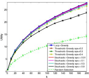
(a) Parkinsons

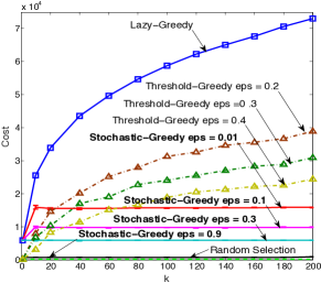
(b) Parkinsons

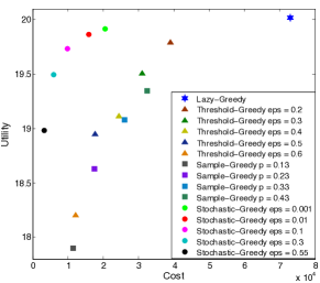
(c) Parkinsons

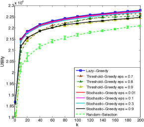
(d) Images 10K

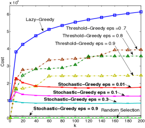
(e) Images 10K

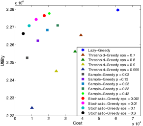
(f) Images 10K

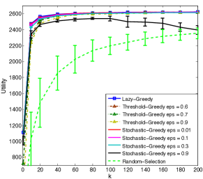
(g) Water Network

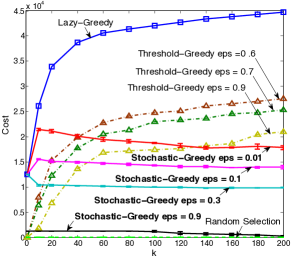
(h) Water Network

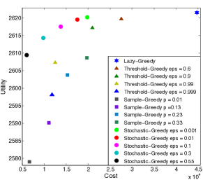
(i) Water Network

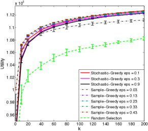
(j) Images 50K

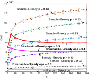
(k) Images 50K

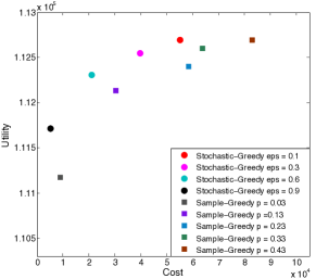
(l) Images 50K

Figure 1: Performance comparisons. a), d) g) and j) show the performance of all the algorithms for different values of $k$ on Parkinsons Telemonitoring, a set of 10,000 Tiny Images, Water Network, and a set of 50,000 Tiny Images respectively. b), e) h) and k) show the cost of all the algorithms for different values of $k$ on the same datasets. c), f), i), l) show the utility obtained versus cost for a fixed $k=200$.

Conclusion

We have developed the first linear time algorithm Stochastic-Greedy with no dependence on $k$ for cardinality constrained submodular maximization. Stochastic-Greedy provides a $1-1/e-\epsilon$ approximation guarantee to the optimum solution with only $n\log\frac{1}{\epsilon}$ function evaluations. We have also demonstrated the effectiveness of our algorithm through an extensive set of experiments. As these show, Stochastic-Greedy achieves a major fraction of the function utility with much less computational cost. This improvement is useful even in approaches that make use of parallel computing or decompose the submodular function into simpler functions for faster evaluation. The properties of Stochastic-Greedy make it very appealing and necessary for solving very large scale problems. Given the importance of submodular optimization to numerous AI and machine learning applications, we believe our results provide an important step towards addressing such problems at scale.

Appendix, Analysis

The following lemma gives us the approximation guarantee.

Lemma 2.

Given a current solution $A$, the expected gain of Stochastic-Greedy in one step is at least $\frac{1-\epsilon}{k}\sum_{a\in A^{*}\setminus A}\Delta(a|A)$.

Proof.

Let us estimate the probability that $R\cap(A^{*}\setminus A)\neq\emptyset$. The set $R$ consists of $s=\frac{n}{k}\log\frac{1}{\epsilon}$ random samples from $V\setminus A$ (w.l.o.g. with repetition), and hence

$$\Pr[R\cap(A^{*}\setminus A)=\emptyset] =\left(1-\frac{|A^{*}\setminus A|}{|V\setminus A|}\right)^{s}$$

$$\leq e^{-s\frac{|A^{*}\setminus A|}{|V\setminus A|}}$$

$$\leq e^{-\frac{s}{n}|A^{*}\setminus A|}.\vspace{-3mm}$$

Therefore, by using the concavity of $1-e^{-\frac{s}{n}x}$ as a function of $x$ and the fact that $x=|A^{*}\setminus A|\in[0,k]$, we have

$$\Pr[R\cap(A^{*}\setminus A)\!\neq\!\emptyset]\!\geq\!1-e^{-\frac{s}{n}|A^{*}\setminus A|}\!\geq\!(1-e^{-\frac{sk}{n}})\frac{|A^{*}\setminus A|}{k}.$$

Recall that we chose $s=\frac{n}{k}\log\frac{1}{\epsilon}$, which gives

$$\Pr[R\cap(A^{*}\setminus A)\neq\emptyset]\geq(1-\epsilon)\frac{|A^{*}\setminus A|}{k}.$$ (3)

Now consider Stochastic-Greedy: it picks an element $a\in R$ maximizing the marginal value $\Delta(a|A)$. This is clearly as much as the marginal value of an element randomly chosen from $R\cap(A^{*}\setminus A)$ (if nonempty). Overall, $R$ is equally likely to contain each element of $A^{*}\setminus A$, so a uniformly random element of $R\cap(A^{*}\setminus A)$ is actually a uniformly random element of $A^{*}\setminus A$. Thus, we obtain

$$\mbox{\bf E}[\Delta(a|A)]\!\geq\!\Pr[R\cap(A^{*}\setminus A)\neq\emptyset]\times\frac{1}{|A^{*}\setminus A|}\!\!\sum_{a\in A^{*}\setminus A}\!\!\!\Delta(a|A).$$

Using (3), we conclude that $\mbox{\bf E}[\Delta(a|A)]\geq\frac{1-\epsilon}{k}\sum_{a\in A^{*}\setminus A}\Delta(a|A)$. ∎

Now it is straightforward to finish the proof of Theorem 1. Let $A_{i}=\{a_{1},\ldots,a_{i}\}$ denote the solution returned by Stochastic-Greedy after $i$ steps. From Lemma 2,

$$\mbox{\bf E}[\Delta(a_{i+1}|A_{i})\mid A_{i}]\geq\frac{1-\epsilon}{k}\sum_{a\in A^{*}\setminus A_{i}}\Delta(a|A_{i}).\vspace{-4mm}$$

By submodularity,

$$\sum_{a\in A^{*}\setminus A_{i}}\Delta(a|A_{i})\geq\Delta(A^{*}|A_{i})\geq f(A^{*})-f(A_{i}).$$

Therefore,

$$\mbox{\bf E}[f(A_{i+1})-f(A_{i})\mid A_{i}] =\mbox{\bf E}[\Delta(a_{i+1}|A_{i})\mid A_{i}]$$

$$\geq\frac{1-\epsilon}{k}(f(A^{*})-f(A_{i})).$$

By taking expectation over $A_{i}$,

$$\mbox{\bf E}[f(A_{i+1})-f(A_{i})]\geq\frac{1-\epsilon}{k}\mbox{\bf E}[f(A^{*})-f(A_{i})].$$

By induction, this implies that

$$\mbox{\bf E}[f(A_{k})] \geq\left(1-\left(1-\frac{1-\epsilon}{k}\right)^{k}\right)f(A^{*})$$

$$\geq\left(1-e^{-(1-\epsilon)}\right)f(A^{*})\geq(1-1/e-\epsilon)f(A^{*}).$$

Acknowledgment.

This research was supported by SNF 200021-137971, ERC StG 307036, a Microsoft Faculty Fellowship, and an ETH Fellowship.

References

- [Badanidiyuru and Vondrák 2014] Badanidiyuru, A., and Vondrák, J. 2014. Fast algorithms for maximizing submodular functions. In SODA, 1497–1514.
- [Badanidiyuru et al. 2014] Badanidiyuru, A.; Mirzasoleiman, B.; Karbasi, A.; and Krause, A. 2014. Streaming submodular optimization: Massive data summarization on the fly. In KDD.
- [Blelloch, Peng, and Tangwongsan 2011] Blelloch, G. E.; Peng, R.; and Tangwongsan, K. 2011. Linear-work greedy parallel approximate set cover and variants. In SPAA.
- [Chierichetti, Kumar, and Tomkins 2010] Chierichetti, F.; Kumar, R.; and Tomkins, A. 2010. Max-cover in map-reduce. In Proceedings of the 19th international conference on World wide web.
- [Dasgupta, Kumar, and Ravi 2013] Dasgupta, A.; Kumar, R.; and Ravi, S. 2013. Summarization through submodularity and dispersion. In ACL.
- [El-Arini and Guestrin 2011] El-Arini, K., and Guestrin, C. 2011. Beyond keyword search: Discovering relevant scientific literature. In KDD.
- [El-Arini et al. 2009] El-Arini, K.; Veda, G.; Shahaf, D.; and Guestrin, C. 2009. Turning down the noise in the blogosphere. In KDD.
- [Feige 1998] Feige, U. 1998. A threshold of ln n for approximating set cover. Journal of the ACM.
- [Golovin and Krause 2011] Golovin, D., and Krause, A. 2011. Adaptive submodularity: Theory and applications in active learning and stochastic optimization. Journal of Artificial Intelligence Research.
- [Gomes and Krause 2010] Gomes, R., and Krause, A. 2010. Budgeted nonparametric learning from data streams. In ICML.
- [Guillory and Bilmes 2011] Guillory, A., and Bilmes, J. 2011. Active semi-supervised learning using submodular functions. In UAI. AUAI.
- [Kaufman and Rousseeuw 2009] Kaufman, L., and Rousseeuw, P. J. 2009. Finding groups in data: an introduction to cluster analysis, volume 344. Wiley-Interscience.
- [Kempe, Kleinberg, and Tardos 2003] Kempe, D.; Kleinberg, J.; and Tardos, E. 2003. Maximizing the spread of influence through a social network. In Proceedings of the ninth ACM SIGKDD.
- [Krause and Guestrin 2005] Krause, A., and Guestrin, C. 2005. Near-optimal nonmyopic value of information in graphical models. In UAI.
- [Krause and Guestrin 2011] Krause, A., and Guestrin, C. 2011. Submodularity and its applications in optimized information gathering. ACM Transactions on Intelligent Systems and Technology.
- [Krause et al. 2008] Krause, A.; Leskovec, J.; Guestrin, C.; VanBriesen, J.; and Faloutsos, C. 2008. Efficient sensor placement optimization for securing large water distribution networks. Journal of Water Resources Planning and Management 134(6):516–526.
- [Kumar et al. 2013] Kumar, R.; Moseley, B.; Vassilvitskii, S.; and Vattani, A. 2013. Fast greedy algorithms in mapreduce and streaming. In SPAA.
- [Leskovec et al. 2007] Leskovec, J.; Krause, A.; Guestrin, C.; Faloutsos, C.; VanBriesen, J.; and Glance, N. 2007. Cost-effective outbreak detection in networks. In KDD, 420–429. ACM.
- [Lin and Bilmes 2011] Lin, H., and Bilmes, J. 2011. A class of submodular functions for document summarization. In North American chapter of the Assoc. for Comp. Linguistics/Human Lang. Tech.
- [Minoux 1978] Minoux, M. 1978. Accelerated greedy algorithms for maximizing submodular set functions. Optimization Techniques, LNCS 234–243.
- [Mirzasoleiman et al. 2013] Mirzasoleiman, B.; Karbasi, A.; Sarkar, R.; and Krause, A. 2013. Distributed submodular maximization: Identifying representative elements in massive data. In Neural Information Processing Systems (NIPS).
- [Nemhauser and Wolsey 1978] Nemhauser, G. L., and Wolsey, L. A. 1978. Best algorithms for approximating the maximum of a submodular set function. Math. Oper. Research.
- [Nemhauser, Wolsey, and Fisher 1978] Nemhauser, G. L.; Wolsey, L. A.; and Fisher, M. L. 1978. An analysis of approximations for maximizing submodular set functions - I. Mathematical Programming.
- [Ostfeld et al. 2008] Ostfeld, A.; Uber, J. G.; Salomons, E.; Berry, J. W.; Hart, W. E.; Phillips, C. A.; Watson, J.-P.; Dorini, G.; Jonkergouw, P.; Kapelan, Z.; et al. 2008. The battle of the water sensor networks (bwsn): A design challenge for engineers and algorithms. Journal of Water Resources Planning and Management 134(6):556–568.
- [Rodriguez, Leskovec, and Krause 2012] Rodriguez, M. G.; Leskovec, J.; and Krause, A. 2012. Inferring networks of diffusion and influence. ACM Transactions on Knowledge Discovery from Data 5(4):21:1–21:37.
- [Sipos et al. 2012] Sipos, R.; Swaminathan, A.; Shivaswamy, P.; and Joachims, T. 2012. Temporal corpus summarization using submodular word coverage. In CIKM.
- [Torralba, Fergus, and Freeman 2008] Torralba, A.; Fergus, R.; and Freeman, W. T. 2008. 80 million tiny images: A large data set for nonparametric object and scene recognition. IEEE Trans. Pattern Anal. Mach. Intell.
- [Tsanas et al. 2010] Tsanas, A.; Little, M. A.; McSharry, P. E.; and Ramig, L. O. 2010. Enhanced classical dysphonia measures and sparse regression for telemonitoring of parkinson’s disease progression. In IEEE Int. Conf. Acoust. Speech Signal Process.
- [Wei et al. 2013] Wei, K.; Liu, Y.; Kirchhoff, K.; and Bilmes, J. 2013. Using document summarization techniques for speech data subset selection. In HLT-NAACL, 721–726.
- [Wei, Iyer, and Bilmes 2014] Wei, K.; Iyer, R.; and Bilmes, J. 2014. Fast multi-stage submodular maximization. In ICML.