Cognitive Learning of Statistical Primary Patterns via Bayesian Network

Abstract

In cognitive radio (CR) technology, the trend of sensing is no longer to only detect the presence of active primary users. A large number of applications demand for more comprehensive knowledge on primary user behaviors in spatial, temporal, and frequency domains. To satisfy such requirements, we study the statistical relationship among primary users by introducing a Bayesian network (BN) based framework. How to learn such a BN structure is a long standing issue, not fully understood even in the statistical learning community. Besides, another key problem in this learning scenario is that the CR has to identify how many variables are in the BN, which is usually considered as prior knowledge in statistical learning applications. To solve such two issues simultaneously, this paper proposes a BN structure learning scheme consisting of an efficient structure learning algorithm and a blind variable identification scheme. The proposed approach incurs significantly lower computational complexity compared with previous ones, and is capable of determining the structure without assuming much prior knowledge about variables. With this result, cognitive users could efficiently understand the statistical pattern of primary networks, such that more efficient cognitive protocols could be designed across different network layers.

I Introduction

Since the terminology was coined in 1999 [1], cognitive radio (CR) has been developed for more than fifteen years, which has drawn attention from both academic and industrial communities since it is intended to enable smart use of the scarce spectrum resource with the initial objective of maximizing spectrum utilization. Recently, cognitive network design goes beyond spectrum utilization and target at broader network objectives such as higher quality of service, lower energy cost, etc. To achieve such new objectives, the statistical knowledge on the primary network status becomes necessary [2] for resource management and system control, which gets us closer to the ideal CR operation that integrates spectrum sensing, environment learning, statistical reasoning, and predictive acting. This will go beyond most of the existing CR sensing literature, which usually focus on detecting the presence of primary users only [3, 4, 5].

In practice, the network behavior is impacted by many factors which may change dynamically, such that the uncertainty of a network cannot be priorly represented by a certain statistical distribution. To cope with such an issue, the statistical machine learning methodology becomes a feasible solution for understanding the network activity pattern. In this paper, we introduce the Bayesian network (BN) [6] structure learning method to obtain the statistical primary networking pattern, via observing the on/off status of primary base stations. The Bayesian model has been well known in the field of artificial intelligence (AI) [7]. When considering the probability and uncertainty, BN is a distinct technique for modeling the complex interaction among real world facts [8]. In particular, the BN structure learning is an effective new modeling tool in both spatial and temporal domains. However, the associated computational complexity is high since it needs to evaluate the dependence between each pair of variables in a target system and compute the corresponding conditional probability table [7], which becomes the major drawback in applying BN structure learning. In this paper, we focus on reducing the computational load for efficiently learning the statistical behavior patterns of primary users.

For BN structure learning, the related algorithms could be sorted into two categories. One is to use heuristic searching to construct a probable model and then evaluate it by a scoring function [10]. The structure with the highest score is preferred as the learning outcome. The score-based approach of learning BNs has been proven as a NP-hard problem [11]. The other one is to use conditional independence test to measure every possible dependence relationships one by one, and then determine the structure based on the evaluated dependence. In [12], the authors show a much more efficient approach to learn the ordered BN by using mutual information to check the dependence of any possible pairs of nodes. However, this approach cannot be adaptively adjusted when the number of variable changes. To overcome the drawbacks of the current learning methods, we propose a structure learning algorithm based on a completely connected graph and the conditional mutual information, which could efficiently learn both the structure and the corresponding conditional probability table. In particular, each pair of variables in the BN is defined with a generalized relationship where the independence case is unified as the weakest dependence case. As a result, the BN network structure is completely connected. Accordingly, the network structure becomes very regular, such that the conditional mutual information based learning could be formulated as a sequence of closed-form function evaluations. With this, our learning algorithm not only has the same computational overhead as that in [12], but can also dynamically adapt to different numbers of variables. Moreover, for further reducing the computational complexity, we simplify the conditional mutual information function and explore the prior knowledge that the CR sensing results are binary.

Besides the complexity problem, there are some special issues in learning BN structure in the context of CR, due to the lack of collaboration from the primary user side. In conventional learning cases, many existing works assume the number of variables and their related observations are usually prior knowledge， and hence only focus on learning the structure among the variables. However, in CR, the observations are usually collected without recording the correct time epoch, causing the observation to be unidentifiable on which time that it belongs to. This is mainly due to the fact that the statistical period of the BN structure, which reflects the temporal pattern, is not known a priori. In essence, the above issues belong to the unsupervised classification problem, with a new challenge to consider the missing time period. To address this, we propose a blind variable identification algorithm, combining with the proposed structure learning algorithm, to learn the period via the fast Fourier transformation (FFT). In conclusion, the proposed structure and period learning algorithms constitute a complete BN structure learning scheme, by which CR could understand the statistical pattern of primary base stations in both spatial and temporal domains.

The remainder of the paper is organized as follows. In Section II, the system model is presented in details. Section III briefly introduces the relationship between the BN method and the wireless communication problem in CR. In Section IV, an efficient algorithm is proposed for jointly learning the structure and the corresponding conditional probability table. In Section V, an algorithm is proposed to obtain the statistical period of BN structure. In Section VI, the simulation and learning results are presented to validate the proposed scheme. Finally, we conclude the paper in Section VII.

II System Model

Our system model consists of a primary cellular network and multiple secondary sensors over an observation area, of which the detailed specifications are given as follows.

The primary cellular network consists of several primary base stations and multiple mobile primary users. The observation area consists of the cells and a road as illustrated in Fig. 1, where we consider the mobile primary users only moving along a one-way (from right to left) road for our case of study. The arrival of the users at the entrance of the road follows a Poisson process. The arrived mobile users pass along the road at a speed generated by a uniform distribution. Once the mobile users move out the road, they are no longer observed. Additionally, the primary network obeys the following setup: 1) The primary base stations are located based on a pre-designed network deployment plan (i.e., at the centers of the cells); 2) the primary users share a single channel and access a primary base station depending on which cell they are located geographically; 3) an ideal TDMA-based multiple access (MAC) scheme is adopted, and the arrival and departure of primary data traffic at each user follow a Poisson process and an exponential service law, respectively. Hence, the on/off status of a primary base station is determined by the overall data traffic generated from the mobile primary users in its cell (here we only consider the uplink transmissions).

A cognitive secondary sensor is installed very close to each primary base station, which implies that the accuracy of sensing could be assumed perfect, such that no sensing errors are considered in this paper. The secondary sensors sense the on/off status of primary base stations periodically in a synchronous fashion. Let set $\mathbb{M}:=\{1,2,\cdots,M\}$ denote the observed primary base stations, and set $\mathbb{T}:=\{1,2,\cdots,T\}$ denote the sequence of time epoch $t$, $t\in{\mathbb{T}}$. In addition, let $f_{i,t}$ be a variable denoting the state of the $i$-th primary base station at time $t$, and $f_{i,t}\in\mathbb{O}:=\{0,1\}$, where $0$ and $1$ represent the off and on statuses respectively.

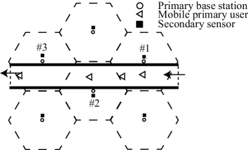
Figure 1: System Diagram

III Cognitive Bayesian Network

In CR, as we argued before, it is valuable to know the statistical behavior of the primary network. By exploring such knowledge, the secondary network could exploit the idle spectrum resource more efficiently and more broadly. In our setup, each secondary sensor could obtain a number of observations (or samples) about the on/off status of the observed primary base station, which is the key element of the primary network. The existing works with respect to CR sensing have been mainly focused on the busy/idle status of a particular spectrum hole by observing a specific primary base station. Contrastingly, our objective is to learn the statistical pattern of the spatial and temporal behavior of multiple networked primary base stations by mining the obtained observations over the whole network across different time epochs. To achieve our objective, BN structure learning is deployed as the key methodology. The BN framework has been known in the field of artificial intelligence and exploited in different expert systems to model complex interactions among causes and consequences, while BN structure learning aims to derive and quantify the complex interaction from data.

III-A Bayesian Network Approach

With BN, the spatial and temporal interactions among primary base stations are expressed by a directed graph $\mathbb{G}=(\mathbb{V},\mathbb{E})$, where $\mathbb{V}$ is a finite, nonempty set whose elements are called the nodes denoting the variable $f_{i,t}$, and $\mathbb{E}$ is a set of directed lines called the edges connecting the pairs of distinct elements in $\mathbb{V}$. If there is a directed edge from $f_{i_{1},t_{1}}$ to $f_{i_{2},t_{2}}$ where $f_{i_{1},t_{1}},f_{i_{2},t_{2}}\in\mathbb{E}$, it means that $f_{i_{2},t_{2}}$ is impacted by $f_{i_{1},t_{1}}$ i.e., $f_{i_{2},t_{2}}$ depends on $f_{i_{1},t_{1}}$. In BN analysis, such a directional relationship is generally expressed by a conditional probability $P(f_{i_{2},t_{2}}|f_{i_{1},t_{1}})$. For the graphical BN, it has a distinguishing feature that: For an arbitrary $f_{i,t}\in\mathbb{V}$, it is conditionally independent of the set of all other indirectly connected nodes given the set of all directly connected nodes. Apparently, if we have the complete knowledge on $(\mathbb{V},\mathbb{E})$ together with all the values of $P(f_{i_{2},t_{2}}|f_{i_{1},t_{1}})$, the statistical pattern of the network behavior is readily available.

III-B BN Structure Learning in CR

As explained above, for quantifying the BN and the related graph from observations, we need to determine both the variables (nodes) and the dependence of each pair of variables (edge). In many applications, the number of variables is priorly known. Hence, most of learning results mainly focus on how to learn the edges efficiently. In our CR scenario, since the observations are collected from the deployed sensors, it is easy to identify $\mathbb{M}$ for the range of $i$ in $f_{i,t}$. However, due to the randomness of the primary user number, speed, and traffic, the temporal information about $\mathbb{T}$, which defines the range for $t$ of $f_{i,t}$, is not directly known. Thus, BN learning in CR not only needs to efficiently mine the relationship and interaction among the variables, but also has to identify the temporal scale $T$ of BN. Since $T$ is not known, we cannot simply sort the observations into the corresponding nodes. Hence, the unknown time scale $T$ becomes a critical issue in the proposed CR BN learning. In machine learning language, such an issue belongs to the unsupervised classification problem, which is widely considered difficult.

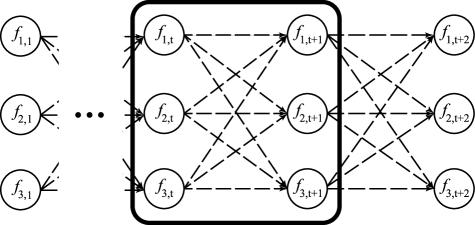
Figure 2: Learning CBN Structure, $M=3$. The dashed line means that the value of an edge has not been determined.

For edge learning, the traditional learning methods are based on scoring or dependence checking functions. Given a scoring function, the computational complexity of determining the BN structure increases exponentially when the number of variables increases. The score-based approach for learning Bayesian networks has been shown NP-hard [11], which is a key challenge in the learning community. Recently, a relatively efficient way to learn an ordered BN is given in [12] by using the conditional mutual information to check the dependence between any possible pair of nodes. Formally, the conditional mutual information is defined as

$$I(X;Y|Z)= \sum_{z\in Z}\sum_{y\in Y}\sum_{x\in X}P_{X,Y,Z}(x,y,z)$$ (1)

$$\times\log\frac{P_{Z}(z)P_{X,Y,Z}(x,y,z)}{P_{X,Z}(x,z)P_{Y,Z}(y,z)},$$

which is a measure of the mutual dependence between variables $X$ and $Y$ given variable $Z$, where the marginal, joint, and/or conditional probability mass functions are denoted by $P$ with appropriate subscripts. Evidently, this method demands for multiple nested for-loops for implementation, and the number of for-loops is determined by the number of variables in the BN. Hence, this method is not directly applicable for the online learning case where the number of variables may be time-varying. Moreover, in [12], the conditional mutual information checking is performed for every combination of all possible parent nodes of $X$. In other words, $I(f_{i,t};f_{i,t-1}|\mathbb{F}_{t-1})$ is computed for all $\mathbb{F}_{t-1}$ where $\mathbb{F}_{t-1}$ denotes the $k$-combination of set $\{f_{1,t-1},\cdots,f_{M,t-1}\}$, $k\in\mathbb{M}$. The combination based checking introduces the huge computational overhead.

III-C Cognitive Bayesian Network Learning

Considering the unknown $T$ and the high computational complexity issues, we propose a BN model for our CR sensing case, and term it as cognitive BN (CBN). The CBN has four characteristics: 1) It is a first-order BN and its nodes are ordered in the temporal domain; 2) its structure is completely connected which means $\forall i\in\mathbb{M},\forall t\in\mathbb{T}\backslash\{1\}$, there exists an edge between any $f_{i,t}$ and $f_{i,t-1}$; 3) the observation of each variable is binary; 4) it has an unknown operation period. Here, “ordered in the temporal domain” means that for a given $i$, $f_{i,t},f_{i,t+1}\cdots$ are ordered in $t,t+1\cdots$. Characteristics 3 and 4 are two direct outcomes from the system model. Thus we only explain characteristics 1 and 2 below.

In our system model, the user movement and data service behaviors of primary users at the current time epoch $t$ could be solely determined by the system states in the former time epoch $t-1$. In other words, our system model has the first-order Markov property, which has been adopted previously [13]. In [13], it is shown that a wireless communication network could be represented by a Markov state transition system. Hence, we have characteristic 1 in our model, which leads to huge complexity reduction in checking the multiple ordered nodes. Next, we explain characteristic 2 in detail, which is unique and critical in further reducing the computational burden.

When learning the edges, the conventional approaches usually consider the edges either existing or absent, by analyzing the directed dependence that is based on the empirical probabilities generated from observations, where the edge weight could be considered as a bi-level quantization of the directed dependence [14]. In contrast, this paper first considers the existence of every possible edge in the first-order BN model, and then quantifies the existence with an analog value to reflect the dependence level between any two nodes. In other words, we consider independence as an extreme case of dependence with edge value $=0$, which implies that each pair of variables in the CBN has a generalized relationship. Based on such an approach, the CBN has a completely connected structure that is highly regular, as shown in Fig. 2. In the next section, we show that, by exploring the regularity of the CBN structure, both the analog-valued edges and the conditional probability table could be learned efficiently.

IV Efficient Learning in CBN

In this section, we propose an efficient learning algorithm which could correctly work under an arbitrary period $T$, while the problem of an unknown $T$ is studied in the next section. As explained before, high computational complexity is a critical issue in BN structure learning. It has been shown [12] that the mutual information check based approach leads to the desired efficiency; but it cannot handle a dynamic number of variables. Here, we proposed an efficient learning algorithm of the same complexity as the $I(X;Y|Z)$ based method, and can cope with the varying number of variables.

When employing the conditional mutual information, every possible edge will be checked in turn. In other words, the number of possible edges affects the learning overhead. Recall that our CBN is a first-order BN and ordered in the temporal domain. It means that, in CBN, the direction of edges is known and the edge only connects the adjacent nodes for a given $i$ in $f_{i,t}$ as shown in Fig. 2. Hence, the computational complexity of learning such a CBN is proportional to learning a subgraph enclosed by the bold-line rectangle in Fig. 2. If we do not consider the direction of edges, this subgraph is called a clique in a Markov network. For the clarity of expression, we here call the targeted subgraph as a C-clique. According to characteristic 1, the number of edges in a CBN is $T$ times as that in a C-clique. Apparently, the computational complexity of learning CBN is linearly proportional to the overhead of learning a C-clique. Hence, in the following study, we focus on how to efficiently learn a C-clique.

IV-A Learning a C-clique by Conventional Methods

Before introducing our idea, we need to show how the current approaches learn a CBN by using the conditional mutual information check, which is helpful for us to understand the computational complexity of learning a C-clique with the proposed algorithm. In conventional methods, when learning the edges in a C-clique, we need to determine the existence of possible edges one by one. For example, to check the edge between $f_{1,t}$ and $f_{1,t+1}$ with a realization of $M=3$ as shown in Fig. 2, the corresponding conditional mutual information $I(f_{1,t};f_{1,t+1}|\mathbb{F}_{t})$ is performed by three times for $\mathbb{F}_{t}:=\{f_{2,t}\}$, $\mathbb{F}_{t}:=\{f_{3,t}\}$, and $\mathbb{F}_{t}:=\{f_{2,t},f_{3,t}\}$.

Actually, according to information theory, there exists

$$I(f_{i,t};f_{i,t+1}|\mathbb{F}_{t}) =I(f_{i,t};f_{i,t+1}|\mathbb{F}_{p,t},\mathbb{F}_{t}\backslash\mathbb{F}_{p,t})$$ (2)

$$=I(f_{i,t};f_{i,t+1}|\mathbb{F}_{p,t})$$

where $\mathbb{F}_{t}:=\{f_{1,t},f_{2,t},\cdots\}$ is a set containing all nodes at $t$, and $\mathbb{F}_{p,t}\subset\mathbb{F}_{t}$ is a set containing all parent nodes of $f_{i,t+1}$ at $t$. (2) means that it is not necessary to check the mutual information conditioned on every possible $\mathbb{F}_{t}$. To utilize such results, the proposed completely connected structure shows a distinct merit that we only need perform the following checking once,

$$I(f_{1,t};f_{1,t+1}|f_{2,t},f_{3,t})$$ (3)

$$= \sum_{f_{1,t}}\sum_{f_{2,t}}\sum_{f_{3,t}}\sum_{f_{1,t+1}}P(f_{1,t},f_{2,t},f_{3,t},f_{1,t+1})$$

$$\times\log\frac{P(f_{2,t},f_{3,t})P(f_{1,t},f_{2,t},f_{3,t},f_{1,t+1})}{P(f_{1,t},f_{2,t},f_{3,t})P(f_{1,t+1},f_{2,t},f_{3,t})},$$

where each probability is estimated by an empirical probability.

On the other hand, the computational load of calculating $I(f_{1,t};f_{1,t+1}|f_{2,t},f_{3,t})$ is mainly determined by using the related observations to calculate both the empirical probability $P(f_{1,t},f_{2,t},f_{3,t},f_{1,t+1})$ and the structure of $I(f_{1,t};f_{1,t+1}|f_{2,t},f_{3,t})$ function itself. Apparently, the related computation requires all the realizations of $\{f_{1,t},f_{2,t},f_{3,t},f_{1,t+1}\}$, e.g. $\{f_{1,t}=0,f_{2,t}=0,f_{3,t}=0,f_{1,t+1}=0\}$, $\{f_{1,t}=0,f_{2,t}=0,f_{3,t}=0,f_{1,t+1}=1\}$, $\cdots$, $\{f_{1,t}=1,f_{2,t}=1,f_{3,t}=1,f_{1,t+1}=1\}$. As a result, the computational complexity of measuring an edge depends on computing $2^{(3+1)}$ times of $P(f_{1,t},f_{2,t},f_{3,t},f_{1,t+1})\log\frac{P(f_{2,t},f_{3,t})P(f_{1,t},f_{2,t},f_{3,t},f_{1,t+1})}{P(f_{1,t},f_{2,t},f_{3,t})P(f_{1,t+1},f_{2,t},f_{3,t})}$. In general, since there are $M^{2}$ edges in a C-clique, the computational complexity of learning a C-clique is determined by running $M^{2}2^{(M+1)}$ times of $P(f_{1,t},f_{2,t},f_{3,t},f_{1,t+1})\log\frac{P(f_{2,t},f_{3,t})P(f_{1,t},f_{2,t},f_{3,t},f_{1,t+1})}{P(f_{1,t},f_{2,t},f_{3,t})P(f_{1,t+1},f_{2,t},f_{3,t})}$. Such outcome implies that the computational complexity of learning a C-clique could be reduced by improving the dependency checking function. On the other hand, each term in (3) is actually based on the conditional probability table considering that the C-clique is completely connected. When each term in (3) is estimated by the empirical probabilities, the computational complexity of (3) is proportional to that of computing the conditional probability table. Evidently, if we could efficiently learn the complete conditional probability table and quantify each edge by closed-form expressions and without nested for-loops, the issues of varying variables and high computational complexity will be solved and released, respectively. Based on the above two ideas, we next propose an efficient algorithm based on analyzing the completely connected structure and exploring the fact of binary observations.

IV-B Efficient Learning Algorithm for Conditional Probability Table

As explained before, the efficiency of the mutual information based CBN learning is determined by two factors: the measurement method of dependence and the adaptation to the number of variables. Among the two factors, the latter one plays a leading role. In this subsection, we show our effort to handle the second factor by utilizing characteristic 2 of our CBN.

IV-B1 Completely Connected Structure and Its Benefit

In a completely connected BN, we need to compute $P(f_{i,t}|\text{pa}(f_{i,t}))$, $\forall i\in\mathbb{M}$ and $\forall t\in\mathbb{{T}}$, to obtain the conditional probability table, where $\text{pa}(f_{i,t})$ means $f_{i,t}$’s parents that are the nodes connecting to $f_{i,t}$ directly. From a glance, the completely connected BN is of high computational complexity because of the large number of edges. However, the fact is just the opposite. Since the structure of a completely connected BN is perfectly symmetry, the algorithm of computing the conditional probability table could be designed efficiently, which will be discussed next.

For a variable $f_{i,t}$, consider its related observations contained in a column vector $\boldsymbol{o}_{i,t}$. For brevity, we take $M=2$ along with binary observations to explain our idea, and then extend the related results to a general case with $M\geq 2$. From the perspective of frequentist probability, the empirical conditional probability table of $P(f_{i,t}|\text{pa}(f_{i,t}))$ in a C-clique is given by

$$P(f_{1,t}=1|f_{1,t-1}=1,f_{2,t-1}=1)= \frac{\boldsymbol{o}_{1,t-1}^{T}\circ\boldsymbol{o}_{2,t-1}^{T}}{\boldsymbol{o}_{1,t-1}^{T}\boldsymbol{o}_{2,t-1}}\boldsymbol{o}_{1,t},$$ (4)

where $\circ$ is the Hadamard product,

$$P(f_{1,t}=1|f_{1,t-1}=0,f_{2,t-1}=1)= \frac{\bar{\boldsymbol{o}}_{1,t-1}^{T}\circ\boldsymbol{o}_{2,t-1}^{T}}{\bar{\boldsymbol{o}}_{1,t-1}^{T}\boldsymbol{o}_{2,t-1}}\boldsymbol{o}_{1,t},$$ (5)

where $\bar{\boldsymbol{o}}_{1,t-1}^{T}=1-\boldsymbol{o}_{1,t-1}^{T}$,

$$P(f_{1,t}=1|f_{1,t-1}=1,f_{2,t-1}=0)= \frac{\boldsymbol{o}_{1,t-1}^{T}\circ\bar{\boldsymbol{o}}_{2,t-1}^{T}}{\boldsymbol{o}_{1,t-1}^{T}\bar{\boldsymbol{o}}_{2,t-1}}\boldsymbol{o}_{1,t},$$ (6)

where $\bar{\boldsymbol{o}}_{2,t-1}^{T}=1-\boldsymbol{o}_{2,t-1}^{T}$,

$$P(f_{1,t}=1|f_{1,t-1}=0,f_{2,t-1}=0)= \frac{\bar{\boldsymbol{o}}_{1,t-1}^{T}\circ\bar{\boldsymbol{o}}_{2,t-1}^{T}}{\bar{\boldsymbol{o}}_{1,t-1}^{T}\bar{\boldsymbol{o}}_{2,t-1}}\boldsymbol{o}_{1,t},$$ (7)

$$P(f_{2,t}=1|f_{1,t-1}=1,f_{2,t-1}=1)= \frac{\boldsymbol{o}_{1,t-1}^{T}\circ\boldsymbol{o}_{2,t-1}^{T}}{\boldsymbol{o}_{1,t-1}^{T}\boldsymbol{o}_{2,t-1}}\boldsymbol{o}_{2,t},$$ (8)

$$P(f_{2,t}=1|f_{1,t-1}=0,f_{2,t-1}=1)= \frac{\bar{\boldsymbol{o}}_{1,t-1}^{T}\circ\boldsymbol{o}_{2,t-1}^{T}}{\bar{\boldsymbol{o}}_{1,t-1}^{T}\boldsymbol{o}_{2,t-1}}\boldsymbol{o}_{2,t},$$ (9)

$$P(f_{2,t}=1|f_{1,t-1}=1,f_{2,t-1}=0)= \frac{\boldsymbol{o}_{1,t-1}^{T}\circ\bar{\boldsymbol{o}}_{2,t-1}^{T}}{\boldsymbol{o}_{1,t-1}^{T}\bar{\boldsymbol{o}}_{2,t-1}}\boldsymbol{o}_{2,t},$$ (10)

and

$$P(f_{2,t}=1|f_{1,t-1}=0,f_{2,t-1}=0)= \frac{\bar{\boldsymbol{o}}_{1,t-1}^{T}\circ\bar{\boldsymbol{o}}_{2,t-1}^{T}}{\bar{\boldsymbol{o}}_{1,t-1}^{T}\bar{\boldsymbol{o}}_{2,t-1}}\boldsymbol{o}_{2,t}.$$ (11)

It is easy to see that the empirical conditional probability could be calculated as multiplying the observation $\boldsymbol{o}_{m,t}$ by a regular arithmetic operator denoted by $\mathcal{F}$. We add an index $c$ to $\mathcal{F}$ to express the condition, e.g., $\mathcal{F}_{c}$ with $c=00$ stands for the arithmetic operator under $f_{1,t-1}=0$ and $f_{2,t-1}=0$, such that we have $\mathcal{F}_{00}=\frac{\bar{\boldsymbol{o}}_{1,t-1}^{T}\circ\bar{\boldsymbol{o}}_{2,t-1}^{T}}{\bar{\boldsymbol{o}}_{1,t-1}^{T}\bar{\boldsymbol{o}}_{2,t-1}}$.

From (4)-(7) and (8)-(11), we see that the computation of the conditional probability table is transformed to obtaining the arithmetic operator $\mathcal{F}_{c}$ with every realization of index $c$, where the structure of $\mathcal{F}_{c}$ is very regular, which benefits from characteristic 2 of our CBN. Based on the regularity of $\mathcal{F}_{c}$, the edges no longer need to be learned one by one, which is explained as follows.

IV-B2 Binary Observation based Conditional Probability Table (BbCPT) Learning Algorithm

In CR, the on/off behavior of a primary base station is expressed by a binary value, which leads to our learning algorithm exploring this fact.

Given binary observations, the number of realizations of $c$ is $2^{M}$, based on which we define $x\in\{0,1,\cdots,2^{M}-1\}$. Accordingly, for a given $x$, we could use (12) defined below to generate a corresponding vector $\boldsymbol{c}_{x}$ leading to $c=\boldsymbol{c}_{x}[1]\times\boldsymbol{c}_{x}[2]\times\cdots\times\boldsymbol{c}_{x}[M]$, with

$$\boldsymbol{c}_{x}[i]=\left\lfloor\frac{x}{2^{i-1}}\right\rfloor\backslash 2$$ (12)

where $\backslash$ denotes the modulo operation and $i\in\{1,2,\cdots,M\}$. For example, when $M=2$ and $x=2$, $\boldsymbol{c}_{2}=[1~{}0]$, which means $c=10$. Further, we could generate a matrix $\boldsymbol{C}$ where each row contains a realization of $c$ given $x$:

$$\begin{aligned} \boldsymbol{C}[x,M-i+1]=\left\lfloor\frac{x}{2^{i-1}}\right\rfloor\backslash 2,i\in\mathbb{M}\end{aligned}.$$ (13)

On the other hand, when the observation is binary and we take $M=2$ as in the previous subsection, the numerators of $\mathcal{F}_{11}$, $\mathcal{F}_{10}$, $\mathcal{F}_{01}$, and $\mathcal{F}_{00}$ could be reformulated as

$$\boldsymbol{o}_{1,t-1}^{T}\circ\boldsymbol{o}_{2,t-1}^{T}$$ (14)

$$= \left\lfloor\frac{\boldsymbol{o}_{1,t-1}^{T}+\boldsymbol{o}_{2,t-1}^{T}}{2}\right\rfloor$$

$$= \left\lfloor\frac{1\boldsymbol{o}_{1,t-1}^{T}+1\boldsymbol{o}_{2,t-1}^{T}+0(1-\boldsymbol{o}_{1,t-1}^{T})+0(1-\boldsymbol{o}_{2,t-1}^{T})}{2}\right\rfloor$$

$$= \left\lfloor\frac{\boldsymbol{c}_{3}[\boldsymbol{o}_{1,t-1}^{T},\boldsymbol{o}_{2,t-1}^{T}]+(1-\boldsymbol{c}_{3})(1-[\boldsymbol{o}_{1,t-1}^{T},\boldsymbol{o}_{2,t-1}^{T}])}{2}\right\rfloor,$$

$$\boldsymbol{o}_{1,t-1}^{T}\circ\bar{\boldsymbol{o}}_{2,t-1}^{T}$$ (15)

$$= \left\lfloor\frac{\boldsymbol{o}_{1,t-1}^{T}+(1-\boldsymbol{o}_{2,t-1}^{T})}{2}\right\rfloor$$

$$= \left\lfloor\frac{1\boldsymbol{o}_{1,t-1}^{T}+0\boldsymbol{o}_{2,t-1}^{T}+0(1-\boldsymbol{o}_{1,t-1}^{T})+1(1-\boldsymbol{o}_{2,t-1}^{T})}{2}\right\rfloor$$

$$= \left\lfloor\frac{\boldsymbol{c}_{2}[\boldsymbol{o}_{1,t-1}^{T},\boldsymbol{o}_{2,t-1}^{T}]+(1-\boldsymbol{c}_{2})(1-[\boldsymbol{o}_{1,t-1}^{T},\boldsymbol{o}_{2,t-1}^{T}])}{2}\right\rfloor,$$

$$\bar{\boldsymbol{o}}_{1,t-1}^{T}\circ\boldsymbol{o}_{2,t-1}^{T}$$ (16)

$$= \left\lfloor\frac{(1-\boldsymbol{o}_{1,t-1}^{T})+\boldsymbol{o}_{2,t-1}^{T}}{2}\right\rfloor$$

$$= \left\lfloor\frac{\boldsymbol{c}_{1}[\boldsymbol{o}_{1,t-1}^{T},\boldsymbol{o}_{2,t-1}^{T}]+(1-\boldsymbol{c}_{1})(1-[\boldsymbol{o}_{1,t-1}^{T},\boldsymbol{o}_{2,t-1}^{T}])}{2}\right\rfloor,$$

$$\bar{\boldsymbol{o}}_{1,t-1}^{T}\circ\bar{\boldsymbol{o}}_{2,t-1}^{T}$$ (17)

$$= \left\lfloor\frac{(1-\boldsymbol{o}_{1,t-1}^{T})+(1-\boldsymbol{o}_{2,t-1}^{T})}{2}\right\rfloor$$

$$= \left\lfloor\frac{\boldsymbol{c}_{0}[\boldsymbol{o}_{1,t-1}^{T},\boldsymbol{o}_{2,t-1}^{T}]+(1-\boldsymbol{c}_{0})(1-[\boldsymbol{o}_{1,t-1}^{T},\boldsymbol{o}_{2,t-1}^{T}])}{2}\right\rfloor,$$

respectively. Let $\text{nom}(x)$ and $\text{dnom}(x)$ respectively denote the numerator and denominator of $x$, and $\boldsymbol{\mathcal{F}}$ be a matrix containing all $\mathcal{F}_{c}$’s. Then, we arrive at a simple form for each realization of $\mathcal{F}_{c}$ as

$$\text{nom}(\boldsymbol{\mathcal{F}})$$ (18)

$$= [\text{nom}(\mathcal{F}_{00});\text{nom}(\mathcal{F}_{01});\text{nom}(\mathcal{F}_{10});\text{nom}(\mathcal{F}_{11})]$$

$$= \left\lfloor\frac{\boldsymbol{C}\boldsymbol{O}_{t-1}+(1-\boldsymbol{C})(1-\boldsymbol{O}_{t-1})}{2}\right\rfloor$$

where

$$\boldsymbol{O}_{t-1}=[\boldsymbol{o}_{1,t-1},\boldsymbol{o}_{2,t-1}]^{T},$$ (19)

$$\begin{aligned} \boldsymbol{C}=&\begin{bmatrix}0&0\\ 0&1\\ 1&0\\ 1&1\\ \end{bmatrix}\end{aligned},$$ (20)

with $\boldsymbol{C}$ obtained from (13).

On the other hand, since $\text{nom}(\mathcal{F}_{c})$ is a matrix, we have $\text{dnom}(\mathcal{F}_{c})=\text{nom}(\mathcal{F}_{c})\boldsymbol{1}_{N}$, where $\boldsymbol{1}_{N}$ is a column vector of $N$ ones. Thus, the denominator of $\boldsymbol{\mathcal{F}}$ is given by

$$\text{dnom}(\boldsymbol{\mathcal{F}})=\text{nom}(\boldsymbol{\mathcal{F}})\boldsymbol{1}_{N}.$$ (21)

Extending (18) to an arbitrary value of $M$ yields a general arithmetic operator $\boldsymbol{\mathcal{F}}$,

$$\boldsymbol{\mathcal{F}}= \text{nom}(\boldsymbol{\mathcal{F}})./(\text{nom}(\boldsymbol{\mathcal{F}})\boldsymbol{1}_{N}\otimes\boldsymbol{1}_{N}^{T}),$$ (22)

where $\otimes$ denotes the Kronecker product, and

$$\text{nom}(\boldsymbol{\mathcal{F}})= \left\lfloor\frac{\boldsymbol{C}\boldsymbol{O}_{t-1}+(1-\boldsymbol{C})(1-\boldsymbol{O}_{t-1})]}{M}\right\rfloor,$$ (23)

$$\boldsymbol{O}_{t-1}=[\boldsymbol{o}_{1,t-1},\boldsymbol{o}_{2,t-1},\cdots,\boldsymbol{o}_{M,t-1}]^{T}.$$ (24)

Hence, the empirical conditional probability table could be calculated as

$$\boldsymbol{B}_{t-1} =[\boldsymbol{B}_{1,t-1},\cdots,\boldsymbol{B}_{M,t-1}] =\boldsymbol{\mathcal{F}}\boldsymbol{O}_{t}^{T},$$ (25)

where $\boldsymbol{B}_{i,t-1}$ is a column vector with size $2^{M}$ containing every probability that $f_{i,t}=1$ holds conditioned on $c$.

Consequently, the BbCPT learning algorithm is given by (13) and (22)-(25). When compared with conventional methods, the proposed BbCPT algorithm effectively reduces the number of for-loops to just two for-loops (with matrix computation), and the overall empirical conditional probability table could be obtained by a sequence of closed-form function evaluations efficiently.

At the beginning of this subsection, we stated that the total computational overhead is affected by two factors, with the latter one already discussed in this subsection. Next, we study the first one to show how to efficiently measure the dependence between any pair of two variables in a C-clique.

IV-C Efficient Dependence Measure

Given discrete random variables $X$ with support $\mathcal{X}$ and $Y$ with support $\mathcal{Y}$, the conditional entropy between $X$ and $Y$ is given by

$$H(Y|X)= \sum_{x\in\mathcal{X}}P(x)H(Y|X=x)$$ (26)

$$= -\sum_{x\in\mathcal{X}}P(x)\sum_{y\in\mathcal{Y}}P(y|x)\log P(y|x)$$

$$= \sum_{x\in\mathcal{X},y\in\mathcal{Y}}P(x,y)\log\frac{P(x)}{P(x,y)}.$$

If $Y$ is completely determined by $X$, we have $H(Y|X)=0$; if $Y$ is independent of $X$, we have $H(Y|X)=H(Y)$. Hence, $H(Y|X)\in[0,H(Y)]$ reflects the dependence of $Y$ on $X$. According to information theory, $H(Y|X)+H(X|Y)$ is equivalent to $I(X;Y)$ when measuring the dependence between $X$ and $Y$.

For the CR case where $\mathcal{X}:=\mathbb{O}$ and $\mathcal{Y}:=\mathbb{O}$, the conditional entropy is given by

$$H(Y|X)= -\sum_{x\in\mathcal{X}}P(x)P(y=1|x)\log P(y=1|x)$$ (27)

$$-\sum_{x\in\mathcal{X}}P(x)P(y=0|x)\log P(y=0|x),$$

which is always smaller or equal to $H(Y)$ over all possible $P(x)$. According to (27), there is $H(Y|X)=H(Y)$, i.e., $Y$ independs of $X$, when the following holds.

$$\log{P(y|x=0)}-\log{P(y|x=1)}=0,$$ (28)

for $y=0$ or $1$.

Similarly, we could conclude the same observations for $H(X|Y)$. Evidently, given any values of $P(x)$ and $P(y)$, smaller values of $|\log{P(y=0|x=0)}-\log{P(y=0|x=1)|}$ and $|\log{P(y=1|x=0)}-\log{P(y=1|x=1)}|$ imply larger values of $H(Y|X)$ or $H(X|Y)$, which further implies weaker dependence between $Y$ and $X$. Therefore, we arrive at the following dependence metric, where $D_{p}(y;x)$ is termed as the conditional probability based dependence (CPbD),

$$D_{p}(y;x)= \sum_{y\in\mathbb{O}}|\log{P(y|x=0)}-\log{P(y|x=1)}|$$ (29)

which is symmetric with respect to $P(y=1|x=1)$ and $P(y=1|x=0)$. The proposed CPbD $D_{p}(y;x)$ is not affected by $P(y)$ and $P(x)$, and the value range of $D_{p}(y;x)$ is $[0,+\infty)$. For multiple-variable cases, the CPbD between $x$ and $y$ conditioned on $z$ is given by

$$D_{p}(y;x|z)$$ (30)

$$= \sum_{y,z\in\mathbb{O}}|\log{P(y|z,x=0)}-\log{P(y|z,x=1)}|.$$

Taking the example of $M=2$ in CBN, the CPbD between $f_{1,t-1}$ and $f_{1,t}$ conditional on $f_{2,t-1}$ is given by

$$D_{p}(f_{1,t};f_{1,t-1}|f_{2,t-1})$$ (31)

$$= |\log P(f_{1,t}=1|f_{1,t-1}=1,f_{2,t-1}=1)$$

$$-\log P(f_{1,t}=1|f_{1,t-1}=0,f_{2,t-1}=1)|$$

$$+|\log P(f_{1,t}=1|f_{1,t-1}=1,f_{2,t-1}=0)$$

$$~{}~{}~{}-\log P(f_{1,t}=1|f_{1,t-1}=0,f_{2,t-1}=0)|$$

$$+|\log P(f_{1,t}=0|f_{1,t-1}=1,f_{2,t-1}=1)$$

$$~{}~{}~{}-\log P(f_{1,t}=0|f_{1,t-1}=0,f_{2,t-1}=1)|$$

$$+|\log P(f_{1,t}=0|f_{1,t-1}=1,f_{2,t-1}=0)$$

$$~{}~{}~{}-\log P(f_{1,t}=0|f_{1,t-1}=0,f_{2,t-1}=0)|$$

where each term inside the $\log$ operation could be directly obtained from the conditional probability table derived in Section IV-B. Moreover, each term has a regular relative index $c$ corresponding to the conditional probability table. As shown in the previous subsection, the conditional probability table with respect to $f_{1,t}$ is given as $\boldsymbol{B}_{1,t-1}=[B_{00},B_{01},B_{10},B_{11}]^{T}$. Let $\bar{\boldsymbol{B}}_{1,t-1}=1-{\boldsymbol{B}}_{1,t-1}$; we have $\log\boldsymbol{B}_{1,t-1}=[\log B_{00},\log B_{01},\log B_{10},\log B_{11}]^{T}$ and $\log\bar{\boldsymbol{B}}_{1,t-1}={\log(1-\boldsymbol{B}}_{1,t-1})$. Then $D_{p}(f_{1,t};f_{1,t-1}|f_{2,t-1})$ and $D_{p}(f_{1,t};f_{2,t-1}|f_{1,t-1})$ can be calculated as

$$D_{p}(f_{1,t};f_{1,t-1}|f_{2,t-1})=(\left|\log\boldsymbol{B}_{1,t-1}^{T}\boldsymbol{L}_{1}\right|+\left|\log\bar{\boldsymbol{B}}_{1,t-1}^{T}\boldsymbol{L}_{1}\right|)\boldsymbol{1}_{2},$$ (32)

$$D_{p}(f_{1,t};f_{2,t-1}|f_{1,t-1})=(\left|\log\boldsymbol{B}_{1,t-1}^{T}\boldsymbol{L}_{2}\right|+\left|\log\bar{\boldsymbol{B}}_{1,t-1}^{T}\boldsymbol{L}_{2}\right|)\boldsymbol{1}_{2},$$ (33)

where

$$\begin{aligned} \boldsymbol{L}_{1}=\begin{bmatrix}0&1\\ 1&0\\ 0&-1\\ -1&0\end{bmatrix},\end{aligned}\begin{aligned} \boldsymbol{L}_{2}=\begin{bmatrix}0&1\\ 0&-1\\ 1&0\\ -1&0\end{bmatrix},\end{aligned}$$ (34)

For every possible edge pointing to $f_{1,t}$, the corresponding CPbD is given by

$$[D_{p}(f_{1,t};f_{1,t-1}|f_{2,t-1}),D_{p}(f_{1,t};f_{2,t-1}|f_{1,t-1})]$$ (35)

$$= (\left|\log\boldsymbol{B}_{1,t-1}^{T}\boldsymbol{L}\right|+\left|\log\bar{\boldsymbol{B}}_{1,t-1}^{T}\boldsymbol{L}\right|)\boldsymbol{S}$$

where

$$\boldsymbol{L}=[\boldsymbol{L}_{1},\boldsymbol{L}_{2}],$$ (36)

$$\boldsymbol{S}=\boldsymbol{I}\otimes\boldsymbol{1}_{2}.$$ (37)

Similarly as the above, it is easy to check that $\boldsymbol{L}$ and $\boldsymbol{S}$ obtained for $f_{1,t}$ is still suitable for $f_{2,t}$. Thus, when $M=2$, the CPbD of the C-clique at $t-1$ is given by

$$\boldsymbol{D}_{t-1}= (\left|\log\boldsymbol{B}_{t-1}^{T}\boldsymbol{L}\right|+\left|\log\bar{\boldsymbol{B}}_{t-1}^{T}\boldsymbol{L}\right|)\boldsymbol{S}$$ (38)

where

$$\boldsymbol{D}_{t-1}=\begin{bmatrix}D_{p}(f_{1,t};f_{1,t-1}|f_{2,t-1})&D_{p}(f_{1,t};f_{2,t-1}|f_{1,t-1})\\ D_{p}(f_{2,t};f_{1,t-1}|f_{2,t-1})&D_{p}(f_{2,t};f_{2,t-1}|f_{1,t-1})\end{bmatrix},$$ (39)

$$\boldsymbol{B}_{t-1}=[\boldsymbol{B}_{1,t-1},\boldsymbol{B}_{2,t-1}],$$ (40)

$$\boldsymbol{L}=[\boldsymbol{L}_{1},\boldsymbol{L}_{2}],$$ (41)

$$\boldsymbol{S}=\boldsymbol{I}\otimes\boldsymbol{1}_{2}.$$ (42)

In our system model, the behavior of each primary station follows a same birth-death process, which can be formulated by a Bayesian graph containing two nodes. It means that if we only study the statistical pattern of one base station, the related Bayesian structure consists of one edges and two nodes which means $T=1$. Therefore, the value of $D_{p}(f_{1,t};f_{1,t-1}|f_{2,t-1})$ and $D_{p}(f_{2,t};f_{2,t-1}|f_{1,t-1})$ are same and keep constant over every C-clique of a whole BN graph which expresses the pattern of $M$ primary base stations. On the other hand, the limited number of observations leads that the empirical $D_{p}(f_{1,t};f_{1,t-1}|f_{2,t-1})$ and $D_{p}(f_{2,t};f_{2,t-1}|f_{1,t-1})$ are different. Hence, we normalize the entries in $\boldsymbol{D}_{t-1}$ normalized as follows for reflecting the spatial relationship clearly.

$$\bar{\boldsymbol{D}}_{t-1}= \Lambda^{-1}(\boldsymbol{D}_{t-1})\boldsymbol{D}_{t-1}$$ (43)

$$= \begin{bmatrix}\frac{D_{p}(f_{1,t};f_{1,t-1}|f_{2,t-1})}{D_{p}(f_{1,t};f_{1,t-1}|f_{2,t-1})}&\frac{D_{p}(f_{1,t};f_{2,t-1}|f_{1,t-1})}{D_{p}(f_{1,t};f_{1,t-1}|f_{2,t-1})}\\ \frac{D_{p}(f_{2,t};f_{1,t-1}|f_{2,t-1})}{D_{p}(f_{2,t};f_{2,t-1}|f_{1,t-1})}&\frac{D_{p}(f_{2,t};f_{2,t-1}|f_{1,t-1})}{D_{p}(f_{2,t};f_{2,t-1}|f_{1,t-1})}\end{bmatrix},$$

where $\Lambda(\boldsymbol{D}_{t-1})$ denotes the diagonal matrix with the same main diagonal as $\boldsymbol{D}_{t-1}$.

Consequently, for an arbitrary $M$, the normalized CPbD of C-clique at $t-1$ is given by

$$\bar{\boldsymbol{D}}_{t-1}= \Lambda^{-1}(\boldsymbol{D}_{t-1})\boldsymbol{D}_{t-1},$$ (44)

where

$$\boldsymbol{D}_{t-1}= (\left|\log\boldsymbol{B}_{t-1}^{T}\boldsymbol{L}\right|+\left|\log\bar{\boldsymbol{B}}_{t-1}^{T}\boldsymbol{L}\right|)\boldsymbol{S},$$ (45)

$$\boldsymbol{B}_{t-1}=[\boldsymbol{B}_{1,t-1},\boldsymbol{B}_{2,t-1},\cdots,,\boldsymbol{B}_{M,t-1}],$$ (46)

$$\boldsymbol{S}=\boldsymbol{I}\otimes\boldsymbol{1}_{M}.$$ (47)

It is worth emphasizing that matrix $\boldsymbol{L}$ does not depend on the number of C-cliques, but only on the number of variables in one C-clique. Hence, matrix $\boldsymbol{L}$ only needs to be computed once for a given $M$. It could be computed offline prior to the online CBN learning. This paper does not study the optimal approach to obtain $\boldsymbol{L}$; alternatively, we provide a feasible method to arrive at $\boldsymbol{L}$, given in Table I.

TABLE I: Algorithm of Obtaining $\boldsymbol{L}$.

1)	for $m=1:1:M$
2)	$\boldsymbol{e}_{1}=\boldsymbol{0}_{2^{m}\times 1}$, $\boldsymbol{e}_{1}[2^{m},1]=-1$, $\boldsymbol{e}_{1}[2^{m}/2,1]=1$,
3)	generate a circulant matrix $\boldsymbol{e}$ based on $\boldsymbol{e}_{1}^{T}$,
	each row is a backward shifting of $\boldsymbol{e}_{1}^{T}$,
4)	$\boldsymbol{l}_{1}=\boldsymbol{e}[1:m,:]^{T}$,
5)	for $n=2:1:m$
6)	$\boldsymbol{l}_{n}=\boldsymbol{I}_{2\times 2}\otimes\boldsymbol{L}_{n-1}$, $\boldsymbol{L}_{n-1}=\boldsymbol{l}_{n-1}$,
7)	end
8)	end
9)	$\boldsymbol{L}=[\boldsymbol{L}_{1},\boldsymbol{L}_{2},\cdots,\boldsymbol{L}_{M}]$.

IV-D Efficient C-clique Learning Procedure

Based on the previously discussed BbCPT and CPbD, the procedure of learning a C-clique is summarized as:

Initialization of $\boldsymbol{C}$, $\boldsymbol{L}$, and $\boldsymbol{S}$; 1) Obtain the conditional probability table by (22)-(25); 2) Obtain the CPbD of all edges by (44)-(47).

As we have emphasized before, $\boldsymbol{C}$ and $\boldsymbol{L}$ are only required to calculate once according to the number of variables in a C-clique, which means that they could be calculated and stored priorly. When regarding $\boldsymbol{C}$ and $\boldsymbol{L}$ as prior knowledge, the above procedure shows that our learning algorithm is just a sequence of closed-form function evaluations and has a simpler dependence check function compared with that in [12]. Consequently, the proposed learning method has lower computational complexity and is capable of adapting to different numbers of variables. Note that the learned CPbD is a soft measure on the variable dependence, which will be useful in the next section to derive the general CBN learning algorithm. We could also now apply simple binary threshold over CPbD to decide the existence of the edges in the learned clique, as in [12].

V Learning CBN with Unknown $T$

The previous section introduces the CBN learning algorithm with a given $T$. Sometimes, the value of $T$ is not known a priori. For example. we do not know the exact value of $T$ in our CR system model. The uncertainty of $T$ implies that the number of variables in the temporal domain is unknown in the CBN model. Consequently, after a number of observations being collected, we do not exactly know which temporal variables generated the collected observations. In the structure learning literature, observations are usually assumed already associated with different variables correctly. As such, the uncertainty of $T$ is a challenging issue, less studied in the BN community. For this problem, we propose a heuristic but efficient solution as follows.

To estimate $T$, we first formulate this uncertainty issue into a mathematical problem. Let $D_{p}(x)=\sum_{i,k\in{\mathcal{M}}}D_{p}(f_{i,t+x};f_{k,t}|f_{1:M,t}\backslash f_{k,t})$, which is the sum of the dependence measures over all edges between the variables at times $t$ and $t+x$. In addition, let $T_{p}$, $T_{s}$, and $T^{*}$ denote the period of CPbD, the interval between two sequential observations of the same variable, and the minimal value of period $T$, respectively. Note that all the periods in the set $\{T|T=kT^{*},k\in\mathbb{Z}\}$ are feasible for the BN structure (here $\mathbb{Z}$ denotes the positive integer set). But a longer period implies higher computational complexity. Hence, we pick the minimal possible value $T^{*}$ as the optimal choice. For $T^{*}$, it not only needs to ensure that the observations are statistically periodic along the temporal variables but also has to guarantee that the observations of a variable are statistically independent over $T_{s}$. Accordingly, when $N\rightarrow\infty$, the optimal period $T^{*}$ could be obtained by solving

$$T^{*} =\arg\min~{}t$$ (48)

$$\text{st}.~{}~{}~{}~{}~{}~{}~{}~{}t =kT_{p},\text{where}~{}k\in\mathbb{Z},$$

$$t \geq T_{s}^{*}-1,$$

where $T_{s}^{*}=\min\{T_{s}|D_{p}(T_{s})=0\}$.

V-A Learning $T_{s}^{*}$

Specifically, the period $T$ should ensure that the observations of any variable $f_{i,t}$ are statistically independent over $T_{s}$. Regarding our system, the temporal correlation of two observations decreases as their interval increases. Obviously, it is better to set a long enough period $T_{s}$ to ensure the statistically independent condition. However, since the number of available observations $N$ is limited in practice, we choose to estimate $T_{s}$ and $T_{p}$ empirically. It is worth noting that: i) it is impossible to deduce the true probability or distribution of a variable from limited observations, and ii) the empirical statistical information is widely used in real system analysis. From the perspective of both statistics and engineering, the empirical probability is valuable and useful as long as it is close to the true one. In addition, it is impossible to find a feasible value of $T_{s}$ to ensure $D_{p}(T_{s})=0$ using empirical probabilities. Hence, given the finite observations, we propose to obtain the empirical $T_{s}$ by finding the first valley value of the CPbD between $f_{1:M,t}$ and $f_{1:M,t+T_{s}}$, denoted by $\boldsymbol{D}_{t,t+T_{s}}$. Here $f_{1:M,t}$ is a short form for $f_{1,t},\cdots,f_{M,t}$. The pseudo-code of the proposed algorithm denoted by $\mathcal{T}_{s}$ is given in Table II, where $\frac{||\boldsymbol{D}_{p}||_{1}}{T_{s}}$ is the $\boldsymbol{D}_{t,t+T_{s}}$ value averaged over $T_{s}$ and edges.

TABLE II: Pseudo-code of $\mathcal{T}_{s}$.

1)	set $l=2$
2)	for $T_{s}=2:1:2^{l}+1$
	for $t=1:1:T_{s}$
	$\boldsymbol{D}_{p}[t]=\boldsymbol{D}_{t,t+T_{s}}$;
	end
	$\boldsymbol{D}[T_{s}-1]=\frac{||\boldsymbol{D}_{p}||_{1}}{T_{s}}$;
	for $t=2:1:T_{s}-1$
	if $\boldsymbol{D}_{p}[t]\leq\boldsymbol{D}_{p}[t-1]$ and $\boldsymbol{D}_{p}[t]\leq\boldsymbol{D}_{p}[t+1]$,
	then break and output $T_{s}^{*}=t$;
	end
	end
3)	if $T_{s}=2^{l}+1$,
	then set $l=l+1$ and goto 2).

Next, we give our algorithm that obtains $T_{p}$ by exploring the regularity of CPbD.

V-B Learning $T_{p}$

As discussed earlier, the CPbD has the capability of reflecting the dependence between variables. Hence, when finding the correct value of $T_{p}$, the CPbD should demonstrate a certain regularity that could help with learning $T_{p}$. This subsection first shows the existence of CPbD regularity mathematically. We need to emphasize that the observations are assumed to have certain correlation in the user and temporal domains, though we do not know the statistical characteristics of such correlation, since if all observations are independent, there will be no edges in the BN structure. To ensure that the unknown $T_{p}$ could be obtained by learning from the observations, we have the following theoretical results.

First, we derive Proposition 1 and Proposition 2 to show that $P(f_{i,t+1}=1|f_{i,t}=1)$ is regular when considering $T$ as a variable, which means that the calculation of the empirical $P(f_{i,t+1}=1|f_{i,t}=1)$ has a regular pattern either. Let $\mathbb{T}_{f}$ and $\mathbb{T}_{r}$ denote the sets containing the false and true periods respectively. Obviously, there is $\mathbb{T}:=\mathbb{T}_{f}\cup\mathbb{T}_{r}$. And let $\mathbb{Z}_{e}:=\{2k:k~{}\text{is positive integer}\}$ and $\mathbb{Z}_{o}:=\{2k+1:k~{}\text{is positive integer}\}$. Additionally, consider $T_{f}^{\prime}$ is a variable similar as $T_{f}$.

Proposition 1

When $T_{f},T_{f}^{\prime}\in\mathbb{T}_{f}$, $T_{r}\in\mathbb{T}_{r}\cap\mathbb{Z}_{o}$, there exist:

P1.1)

$P(f_{i,t+1}=1|f_{i,t}=1)|_{T=T_{f}}\neq P(f_{i,t+1}=1|f_{i,t}=1)|_{T=T_{r}}$.

P1.2)

$P(f_{i,t+1}=1|f_{i,t}=1)|_{T=T_{f}}=P(f_{i,t+1}=1|f_{i,t}=1)|_{T=T_{f}^{\prime}}$.

Proposition 2

When $T_{f},T_{f}^{\prime}\in\mathbb{T}_{f}$, $T_{r}\in\mathbb{T}_{r}\cap\mathbb{Z}_{e}$, there exist:

P2.1)

$P(f_{i,t+1}=1|f_{i,t}=1)|_{T=T_{f}}\neq P(f_{i,t+1}=1|f_{i,t}=1)|_{T=T_{r}}$.

P2.2)

$P(f_{i,t+1}=1|f_{i,t}=1)|_{T=T_{f}}=P(f_{i,t+1}=1|f_{i,t}=1)|_{T=T_{f}^{\prime}}$ under the condition that $T_{f},T_{f}^{\prime}\in\mathbb{Z}_{e}$.

P2.3)

$P(f_{i,t+1}=1|f_{i,t}=1)|_{T=T_{f}}=P(f_{i,t+1}=1|f_{i,t}=1)|_{T=T_{f}^{\prime}}$ under the condition that $T_{f},T_{f}^{\prime}\in\mathbb{Z}_{o}$.

P2.4)

$P(f_{i,t+1}=1|f_{i,t}=1)|_{T=T_{f}}\neq P(f_{i,t+1}=1|f_{i,t}=1)|_{T=T_{f}^{\prime}}$ under the condition that $T_{f}\in\mathbb{Z}_{o}$ and $T_{f}^{\prime}\in\mathbb{Z}_{e}$.

Proof:

We prove Proposition 1 at first. Let $\{o_{1,1},o_{1,2},\cdots,o_{1,N}\}$ denote the $N$ temporal observations of user-1. Then, given the period $T$, we fold this time series at $T$. For example,

• When $T=2$, we have $\boldsymbol{o}_{1,1}|_{T=2}=[o_{1,1},o_{1,3},o_{1,5},\cdots]^{T}$ and $\boldsymbol{o}_{1,2}|_{T=2}=[o_{1,2},o_{1,4},o_{1,6},\cdots]^{T}$.

• When $T=3$, we have $\boldsymbol{o}_{1,1}|_{T=3}=[o_{1,1},o_{1,4},o_{1,7},\cdots]^{T}$, $\boldsymbol{o}_{1,2}|_{T=3}=[o_{1,2},o_{1,5},o_{1,8},\cdots]^{T}$, and $\boldsymbol{o}_{1,3}|_{T=3}=[o_{1,3},o_{1,6},o_{1,9},\cdots]^{T}$.

• When $T=4$, we have $\boldsymbol{o}_{1,1}|_{T=4}=[o_{1,1},o_{1,5},o_{1,9},\cdots]^{T}$, $\boldsymbol{o}_{1,2}|_{T=4}=[o_{1,2},o_{1,6},o_{1,10},\cdots]^{T}$, $\boldsymbol{o}_{1,3}|_{T=4}=[o_{1,3},o_{1,7},o_{1,11},\cdots]^{T}$, and $\boldsymbol{o}_{1,4}|_{T=4}=[o_{1,4},o_{1,8},o_{1,12},\cdots]^{T}$.

• When $T=5$, there exist $\boldsymbol{o}_{1,1}|_{T=5}=[o_{1,1},o_{1,6},o_{1,11},\cdots]^{T}$, $\boldsymbol{o}_{1,2}|_{T=5}=[o_{1,2},o_{1,7},o_{1,12},\cdots]^{T}$, $\boldsymbol{o}_{1,3}|_{T=5}=[o_{1,3},o_{1,8},o_{1,13},\cdots]^{T}$, $\boldsymbol{o}_{1,4}|_{T=5}=[o_{1,4},o_{1,9},o_{1,14},\cdots]^{T}$, and $\boldsymbol{o}_{1,5}|_{T=5}=[o_{1,5},o_{1,10},o_{1,15},\cdots]^{T}$.

• When $T=6$, there exist $\boldsymbol{o}_{1,1}|_{T=6}=[o_{1,1},o_{1,7},o_{1,13},\cdots]^{T}$, $\boldsymbol{o}_{1,2}|_{T=6}=[o_{1,2},o_{1,8},o_{1,14},\cdots]^{T}$, $\boldsymbol{o}_{1,3}|_{T=6}=[o_{1,3},o_{1,9},o_{1,15},\cdots]^{T}$, $\boldsymbol{o}_{1,4}|_{T=6}=[o_{1,4},o_{1,10},o_{1,16},\cdots]^{T}$, $\boldsymbol{o}_{1,5}|_{T=6}=[o_{1,5},o_{1,11},o_{1,17},\cdots]^{T}$, and $\boldsymbol{o}_{1,6}|_{T=6}=[o_{1,6},o_{1,12},o_{1,18},\cdots]^{T}$.

Accordingly, when $T_{r}=5$, we have

$$P(f_{1,2}=1|f_{1,1}=1,T_{f}=2,T_{r}=5)$$ (49)

$$= \lim_{N\to\infty}\frac{\boldsymbol{o}_{1,1}^{T}\boldsymbol{o}_{1,2}}{\boldsymbol{o}_{1,1}^{T}\boldsymbol{1}}\bigg{|}_{T=T_{f}=2}$$

$$= \lim_{N\to\infty}\frac{\sum_{t=1}^{4}\boldsymbol{o}_{1,t}^{T}\boldsymbol{o}_{1,t+1}+\boldsymbol{o}_{1,5}^{T}S(\boldsymbol{o}_{1,1})}{\left(\sum_{t=1}^{5}\boldsymbol{o}_{1,t}^{T}\right)\boldsymbol{1}}\bigg{|}_{T=T_{r}=5},$$

where $S(.)$ denotes an operation shifting the entries of a vector with a single step circularly,

$$P(f_{1,2}=1|f_{1,1}=1,T_{f}=3,T_{r}=5)$$ (50)

$$= \lim_{N\to\infty}\frac{\boldsymbol{o}_{1,1}^{T}\boldsymbol{o}_{1,2}}{\boldsymbol{o}_{1,1}^{T}\boldsymbol{1}}\bigg{|}_{T=T_{f}=3}$$

$$= \lim_{N\to\infty}\frac{\sum_{t=1}^{4}\boldsymbol{o}_{1,t}^{T}\boldsymbol{o}_{1,t+1}+\boldsymbol{o}_{1,5}^{T}S(\boldsymbol{o}_{1,1})}{\left(\sum_{t=1}^{5}\boldsymbol{o}_{1,t}^{T}\right)\boldsymbol{1}}\bigg{|}_{T=T_{r}=5},$$

$$P(f_{1,2}=1|f_{1,1}=1,T_{f}=4,T_{r}=5)$$ (51)

$$= \lim_{N\to\infty}\frac{\boldsymbol{o}_{1,1}^{T}\boldsymbol{o}_{1,2}}{\boldsymbol{o}_{1,1}^{T}\boldsymbol{1}}\bigg{|}_{T=T_{f}=4}$$

$$= \lim_{N\to\infty}\frac{\sum_{t=1}^{4}\boldsymbol{o}_{1,t}^{T}\boldsymbol{o}_{1,t+1}+\boldsymbol{o}_{1,5}^{T}S(\boldsymbol{o}_{1,1})}{\left(\sum_{t=1}^{5}\boldsymbol{o}_{1,t}^{T}\right)\boldsymbol{1}}\bigg{|}_{T=T_{r}=5},$$

$$P(f_{1,2}=1|f_{1,1}=1,T_{f}=T_{r}=5)~{}~{}~{}~{}~{}~{}~{}~{}~{}~{}~{}~{}~{}~{}$$ (52)

$$= \lim_{N\to\infty}\frac{\boldsymbol{o}_{1,1}^{T}\boldsymbol{o}_{1,2}}{\boldsymbol{o}_{1,1}^{T}\boldsymbol{1}}\bigg{|}_{T=T_{f}=5}.$$

From (49)-(52), it is easy to see that $P(f_{1,2}=1|f_{1,1}=1,T_{f}=2,T_{r}=5)=P(f_{1,2}=1|f_{1,1}=1,T_{f}=3,T_{r}=5)=P(f_{1,2}=1|f_{1,1}=1,T_{f}=4,T_{r}=5)\neq P(f_{1,2}=1|f_{1,1}=1,T_{f}=T_{r}=5)$. By a similar approach, we show that such a relationship holds for general $T_{f}$ and $T_{r}$ (where $T_{r}\in\mathbb{Z}_{o}$) as follows.

• When $T=T_{f}$, there exist $\boldsymbol{o}_{1,1}|_{T=T_{f}}=[o_{1,1},o_{1,1+T_{f}},o_{1,1+2T_{f}},\cdots]^{T}$, $\boldsymbol{o}_{1,2}|_{T=T_{f}}=[o_{1,2},o_{1,2+T_{f}},o_{1,2+2T_{f}},\cdots]^{T}$, $\cdots$, and $\boldsymbol{o}_{1,T_{f}}|_{T=T_{f}}=[o_{1,T_{f}},o_{1,2T_{f}},o_{1,3T_{f}},\cdots]^{T}$.

• When $T=T_{r}$, there exist $\boldsymbol{o}_{1,1}|_{T=T_{r}}=[o_{1,1},o_{1,1+T_{r}},o_{1,1+2T_{r}},\cdots]^{T}$, $\boldsymbol{o}_{1,2}|_{T=T_{r}}=[o_{1,2},o_{1,2+T_{r}},o_{1,2+2T_{r}},\cdots]^{T}$, $\cdots$, and $\boldsymbol{o}_{1,T_{r}}|_{T=T_{r}}=[o_{1,T_{r}},o_{1,2T_{r}},o_{1,3T_{r}},\cdots]^{T}$.

Accordingly, we have

$$\begin{aligned} &\boldsymbol{o}_{1,t_{f}}[n]\boldsymbol{o}_{1,t_{f}+1}[n]\\ =&o_{1,t_{f}+(n-1)T_{f}}o_{1,t_{f}+1+(n-1)T_{f}}\\ =&o_{1,t_{r}+(l-1)T_{r}}o_{1,t_{r}+1+(l-1)T_{r}}\\ =&\begin{cases}\boldsymbol{o}_{1,t_{r}}[l]\boldsymbol{o}_{1,t_{r}+1}[l],\text{when}~{}t_{r}\neq 0\\ \boldsymbol{o}_{1,T_{r}}[l]S(\boldsymbol{o}_{1,1})[l],\text{when}~{}t_{r}=0\\ \end{cases}\end{aligned},$$ (53)

for the numerator, where $n$ and $l$ are indices, $t_{r}$ and $t_{f}$ respectively denote $t|_{T=T_{r}}$ and $t|_{T=T_{f}}$, and

$$\begin{aligned} t_{r}=[t_{f}+(n-1)T_{f}]\backslash T_{r}\end{aligned},$$ (54)

$$\begin{aligned} l=\left\lfloor\frac{t_{f}+(n-1)T_{f}}{T_{r}}\right\rfloor+1\end{aligned}.$$ (55)

On the other hand, for the denominator, there exists $\boldsymbol{o}_{1,t_{f}}[n]=o_{1,t_{f}+(n-1)T_{f}}=o_{1,t_{r}+(l-1)T_{r}}=\boldsymbol{o}_{1,t_{r}}[l]$.

Given $T_{r}\in\mathbb{Z}_{o}$, the modulo operation in (54) leads to $t_{r}\in\{0,1,2,\cdots,T_{r}-1\}$ when $n$ increases. Hence, we could obtain

$$P(f_{1,t+1}=1|f_{1,t}=1,T_{f},T_{r})$$ (56)

$$= \lim_{N\to\infty}\frac{\boldsymbol{o}_{1,t}^{T}\boldsymbol{o}_{1,t+1}}{\boldsymbol{o}_{1,t}^{T}\boldsymbol{1}}\bigg{|}_{T=T_{f}}$$

$$= \lim_{N\to\infty}\frac{\sum_{t=1}^{T_{r}-1}\boldsymbol{o}_{1,t}^{T}\boldsymbol{o}_{1,t+1}+\boldsymbol{o}_{1,T_{r}}^{T}S(\boldsymbol{o}_{1,1})}{\left(\sum_{t=1}^{T_{r}}\boldsymbol{o}_{1,t}^{T}\right)\boldsymbol{1}}\bigg{|}_{T=T_{r}},$$

and then could extend it to the following result,

$$P(f_{i,t+1}=1|f_{i,t}=1,T_{f},T_{r})$$ (57)

$$= \lim_{N\to\infty}\frac{\boldsymbol{o}_{i,t}^{T}\boldsymbol{o}_{i,t+1}}{\boldsymbol{o}_{i,t}^{T}\boldsymbol{1}}\bigg{|}_{T=T_{f}}$$

$$= \lim_{N\to\infty}\frac{\sum_{t=1}^{T_{r}-1}\boldsymbol{o}_{i,t}^{T}\boldsymbol{o}_{i,t+1}+\boldsymbol{o}_{i,T_{r}}^{T}S(\boldsymbol{o}_{i,1})}{\left(\sum_{t=1}^{T_{r}}\boldsymbol{o}_{i,t}^{T}\right)\boldsymbol{1}}\bigg{|}_{T=T_{r}}.$$

When jointly reviewing the first and second equations in (57), it is obvious that $\forall T_{f}\in\mathbb{T}_{f}$, $P(f_{i,t+1}=1|f_{i,t}=1,T_{f},T_{r})$ keeps constant. In other words, $\forall T_{f},T_{f}^{\prime}\in\mathbb{T}_{f}$, $P(f_{i,t+1}=1|f_{i,t}=1,T_{f},T_{r})$ and $P(f_{i,t+1}=1|f_{i,t}=1,T_{f}^{\prime},T_{r})$ have the same value. Hence, P1.1) is proved. On the other hand, we also could see that $P(f_{i,t+1}=1|f_{i,t}=1,T=T_{f})$ and $P(f_{i,t+1}=1|f_{i,t}=1,T=T_{r})$ are different. Consequently, Proposition 1 is proved. Next, we prove Proposition 2.

When $T_{r}=6$, we have

$$P(f_{1,2}=1|f_{1,1}=1,T_{f}=2,T_{r}=6)$$ (58)

$$= \lim_{N\to\infty}\frac{\boldsymbol{o}_{1,1}^{T}\boldsymbol{o}_{1,2}}{\boldsymbol{o}_{1,1}^{T}\boldsymbol{1}}\bigg{|}_{T=T_{f}=2}$$

$$= \lim_{N\to\infty}\frac{\sum_{t\in\{1,3,5\}}\boldsymbol{o}_{1,t}^{T}\boldsymbol{o}_{1,t+1}}{\left(\sum_{t=\{1,3,5\}}\boldsymbol{o}_{1,t}^{T}\right)\boldsymbol{1}}\bigg{|}_{T=T_{r}=6},$$

$$P(f_{1,2}=1|f_{1,1}=1,T_{f}=3,T_{r}=6)$$ (59)

$$= \lim_{N\to\infty}\frac{\boldsymbol{o}_{1,1}^{T}\boldsymbol{o}_{1,2}}{\boldsymbol{o}_{1,1}^{T}\boldsymbol{1}}\bigg{|}_{T=T_{f}=3}$$

$$= \lim_{N\to\infty}\frac{\sum_{t=1}^{5}\boldsymbol{o}_{1,t}^{T}\boldsymbol{o}_{1,t+1}+\boldsymbol{o}_{1,6}^{T}S(\boldsymbol{o}_{1,1})}{\left(\sum_{t=1}^{6}\boldsymbol{o}_{1,t}^{T}\right)\boldsymbol{1}}\bigg{|}_{T=T_{r}=6},$$

$$P(f_{1,2}=1|f_{1,1}=1,T_{f}=4,T_{r}=6)~{}~{}~{}~{}~{}~{}~{}~{}~{}~{}~{}$$ (60)

$$= \lim_{N\to\infty}\frac{\boldsymbol{o}_{1,1}^{T}\boldsymbol{o}_{1,2}}{\boldsymbol{o}_{1,1}^{T}\boldsymbol{1}}\bigg{|}_{T=T_{f}=4}$$

$$= \lim_{N\to\infty}\frac{\sum_{t\in\{1,3,5\}}\boldsymbol{o}_{1,t}^{T}\boldsymbol{o}_{1,t+1}}{\left(\sum_{t=\{1,3,5\}}\boldsymbol{o}_{1,t}^{T}\right)\boldsymbol{1}}\bigg{|}_{T=T_{r}=6},$$

$$P(f_{1,2}=1|f_{1,1}=1,T_{f}=5,T_{r}=6)$$ (61)

$$= \lim_{N\to\infty}\frac{\boldsymbol{o}_{1,1}^{T}\boldsymbol{o}_{1,2}}{\boldsymbol{o}_{1,1}^{T}\boldsymbol{1}}\bigg{|}_{T=T_{f}=5}$$

$$= \lim_{N\to\infty}\frac{\sum_{t=1}^{5}\boldsymbol{o}_{1,t}^{T}\boldsymbol{o}_{1,t+1}+\boldsymbol{o}_{1,6}^{T}S(\boldsymbol{o}_{1,1})}{\left(\sum_{t=1}^{6}\boldsymbol{o}_{1,t}^{T}\right)\boldsymbol{1}}\bigg{|}_{T=T_{r}=6}.$$

From (58)-(61), it is obvious that $P(f_{1,2}=1|f_{1,1}=1,T_{f}=2,T_{r}=6)=P(f_{1,2}=1|f_{1,1}=1,T_{f}=4,T_{r}=6)\neq P(f_{1,2}=1|f_{1,1}=1,T_{f}=3,T_{r}=6)=P(f_{1,2}=1|f_{1,1}=1,T_{f}=5,T_{r}=6)\neq P(f_{1,2}=1|f_{1,1}=1,T_{f}=T_{r}=6)$. By a similar approach, we show that such a relationship holds for general $T_{f}$ and $T_{r}$ (where $T_{r}\in\mathbb{Z}_{e}$) as follows.

When $T_{r}$, $T_{f}\in\mathbb{Z}_{e}$ and $t_{f}\in\mathbb{Z}_{o}$, the modulo operation in (54) leads to $t_{r}\in\{1,3,\cdots,T_{r}-1\}$; when $T_{r}$, $T_{f}\in\mathbb{Z}_{e}$ and $t_{f}\in\mathbb{Z}_{e}$, the modulo operation in (54) leads to $t_{r}\in\{2,4,\cdots,T_{r}\}$. Hence, we have

$$P(f_{i,t+1}=1|f_{i,t}=1,T_{f},T_{r})$$ (62)

$$= \lim_{N\to\infty}\frac{\boldsymbol{o}_{i,t}^{T}\boldsymbol{o}_{i,t+1}}{\boldsymbol{o}_{i,t}^{T}\boldsymbol{1}}\bigg{|}_{T=T_{f}}$$

$$= \begin{cases}\lim_{N\to\infty}\frac{\sum_{t\in\{1,3,\cdots,T_{r}-1\}}\boldsymbol{o}_{i,t}^{T}\boldsymbol{o}_{i,t+1}}{\left(\sum_{t\in\{1,3,\cdots,T_{r}-1\}}\boldsymbol{o}_{i,t}^{T}\right)\boldsymbol{1}}\bigg{|}_{T=T_{r}},\text{when}~{}t|_{T=T_{f}}\in\mathbb{Z}_{o}\\ \lim_{N\to\infty}\frac{\sum_{t\in\{2,4,\cdots,T_{r}\}}\boldsymbol{o}_{i,t}^{T}\boldsymbol{o}_{i,t+1}}{\left(\sum_{t\in\{2,4,\cdots,T_{r}\}}\boldsymbol{o}_{i,t}^{T}\right)\boldsymbol{1}}\bigg{|}_{T=T_{r}},\text{when}~{}t|_{T=T_{f}}\in\mathbb{Z}_{e}\end{cases}.$$

On the other hand, when $T_{r}\in\mathbb{Z}_{e}$ and $T_{f}\in\mathbb{Z}_{o}$, the modulo operation in (54) leads to the same results as (57). Thus, by a similar approach as the proof in the first paragraph below (57), Proposition 2 is proved. ∎

Proposition 1 and Proposition 2 show that there are some regular patterns as the value of $T$ changes. In addition, such patterns are different when the true period is odd or even. Based on the derived two propositions, we have the following two corollaries for the CPbD.

Corollary 1

When $T_{f},T_{f}^{\prime}\in\mathbb{T}_{f}$, $T_{r}\in\mathbb{T}_{r}\cap\mathbb{Z}_{o}$, there exist:

C1.1)

$D(f_{i,t+1};f_{i,t})|_{T=T_{f}}\neq D(f_{i,t+1};f_{i,t})|_{T=T_{r}}$.

C1.2)

$D(f_{i,t+1};f_{i,t})|_{T=T_{f}}=D(f_{i,t+1};f_{i,t})|_{T=T_{f}^{\prime}}$.

Corollary 2

When $T_{f},T_{f}^{\prime}\in\mathbb{T}_{f}$, $T_{r}\in\mathbb{T}_{r}\cap\mathbb{Z}_{e}$, there exist:

C2.1)

$D(f_{i,t+1};f_{i,t})|_{T=T_{f}}\neq D(f_{i,t+1};f_{i,t})|_{T=T_{r}}$.

C2.2)

$D(f_{i,t+1};f_{i,t})|_{T=T_{f}}=D(f_{i,t+1};f_{i,t})|_{T=T_{f}^{\prime}}$ under the condition that $T_{f}$ and $T_{f}^{\prime}$ are odd.

C2.3)

$D(f_{i,t+1};f_{i,t})|_{T=T_{f}}=D(f_{i,t+1};f_{i,t})|_{T=T_{f}^{\prime}}$ under the condition that $T_{f}$ and $T_{f}^{\prime}$ are even.

C2.4)

$D(f_{i,t+1};f_{i,t})|_{T=T_{f}}\neq D(f_{i,t+1};f_{i,t})|_{T=T_{f}^{\prime}}$ under the condition that $T_{f}$ and $T_{f}^{\prime}$ are even and odd respectively.

Proof:

Corollary 1 and Corollary 2 could be proved by jointly applying (29), Proposition 1, and Proposition 2. The detailed proof is omitted here. ∎

Corollary 1 and Corollary 2 show that the CPbD of a CBN given $T_{r}$ is different from that given $T_{f}$. But the CPbD has the same value for all $T_{f}\in\mathbb{T}_{f}$, and has the same value for all $T_{r}\in\mathbb{T}_{r}$. Hence, the CPbD of a CBN is periodical when $T$ monotone increasing. Based on such results, we propose to use the first peak value of the fast Fourier transformation (FFT) of the averaged CPbD between $f_{1:M,t}$ and $f_{1:M,t+T_{s}}$ to find the empirical $T_{p}$. As well-known, the Fourier analysis methodology is a feasible approach to find the periodical information in broad applications. Let nextpow$2(x)$ be a function that returns $y$, which is the maximal integer satisfying $x-2^{y}\geq 0$, and fft($x$) denote the FFT of $x$. The proposed algorithm denoted by $\mathcal{T}_{p}$ is given in Table III.

TABLE III: Pseudo-code of $\mathcal{T}_{p}$.

1)	$l=$nextpow$2(T_{s}^{*})$;
2)	for $T_{s}=2:1:2^{l}+1$
	for $t=1:1:T_{s}$
	$\boldsymbol{D}_{p}[t]=\boldsymbol{D}_{t,t+T_{s}}$;
	end
	$\boldsymbol{D}[T_{s}-1]=\frac{||\boldsymbol{D}_{p}||_{1}}{T_{s}}$;
	end
3)	$\tilde{\boldsymbol{D}}=\text{fft}(\boldsymbol{D})$;
4)	for $u=3:1:2^{l-1}-1$
	if $\tilde{\boldsymbol{D}}[u-1]>\tilde{\boldsymbol{D}}[u-2]$ and $\tilde{\boldsymbol{D}}[u-1]>\tilde{\boldsymbol{D}}[u]$,
	then break and $T_{p}=\max_{n\in\mathbb{Z}}\frac{1}{n(u-1)}$, st. $\frac{1}{n(u-1)}<T_{s}^{*}$;
	end
5)	if $u=2^{l-1}+1$,
	then set $l=l+1$ and go to 2).

V-C Overall CBN Learning Scheme

Based on (48) and the algorithms $\mathcal{T}_{s}$ and $\mathcal{T}_{p}$, the complete learning scheme for the CBN is given in Table IV, by which we could efficiently obtain the CBN with measured edges and the related conditional probability table.

TABLE IV: Pseudo-code of the proposed learning scheme

1)	for $m=1:1:M$
	$\boldsymbol{T}_{s}[m]=\mathcal{T}_{s}|m$;
	end
	$T_{s}=\max_{m}\boldsymbol{T}_{s}[m]$;
2)	set $l=T_{s}$ in 1) of $\mathcal{T}_{s}$ and perform $\mathcal{T}_{s}$ to obtain $T_{s}^{*}$;
3)	perform $\mathcal{T}_{p}$ with $T_{s}^{*}$ to obtain $T_{p}$;
4)	obtain $T$ by using (44)-(47) with $T_{s}^{*}$ and $T_{p}$;
5)	obtain $\boldsymbol{B}_{1:T-1}$ and $\bar{\boldsymbol{D}}_{1:T-1}$ with $T$.

VI Simulation Results

In this section, we first give the comparison of computational complexity between the proposed CPbD algorithm and the conventional one [12]. Then we present the learning outcomes.

VI-A Comparison of Computational Complexity

The computational complexity is evaluated by running the Matlab codes of the proposed algorithm and the conventional one in the same desktop. The corresponding running time is recorded to reflect the real computational cost. In this subsection, the learning complexity is evaluated when considering the CBN structure that only consists of one C-clique, since the learning time of the whole CBN structure is linear to that of a C-clique. Additionally, the impacts of observation numbers and variable numbers are considered for a comprehensive comparison. In our simulations, the observations are generated based on $M$ binomial distributions . The simulated results are presented in Fig. 3 and Fig. 4, where the computational cost is the total running time for obtaining the conditional probability table and the measurement of every edge. It is obvious that the computational cost of the proposed algorithm is much less than the conventional one, especially as the numbers of base stations and observations increase. In particular, when $M=12$ and $N=36000$, the conventional algorithm demands for $502.2$ seconds to learn. It implies that the conventional algorithm is not suitable for online learning even when the number of variables is not large. In Fig. 4, we draw the ratio between the “Conv” and “Prop” costs over $M$, where it is obvious that the proposed scheme is more efficient. According to Fig. 4, the proposed algorithm only requires $1/38$ of the time cost as the conventional one when $M=12$ and $N=36000$. In addition, note that the proposed algorithm could adapt to any number of variables, while the conventional one cannot.

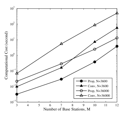
Figure 3: Comparison of computational cost between “Prop” and “Conv”. “Prop” and “Conv” are abbreviations for our proposed scheme and the conventional one proposed in [12], respectively.

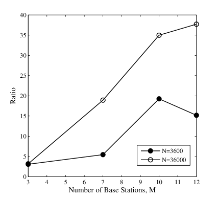
Figure 4: Ratio of the Conv’s computational cost to the Prop’s.

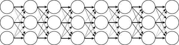
Figure 5: Illustration of learned CBN. The width of edges reflects the magnitude of dependence.

VI-B Learning Outcomes

The simulation scenario is illustrated by Fig. 1, where mobile users move from the right to the left and access one of the three primary base stations according to their locations. The base stations are respectively labeled $\#1$, $\#2$, and $\#3$ from right to left. The simulation configuration is as follows: The arrival of mobile users follows a Poisson distribution with mean $\lambda_{s}=1$; the length of the road is $600$ meters, covered by the three cells; the data traffic arrival rate at each user follows a Poisson distribution with mean $\lambda_{t}=0.002$; the service time of data traffic follows an exponential distribution with a mean of $2$ seconds; and spectrum sensing is performed once per second.

In this paper, we are interested in the relationship among base station activities, which is introduced by the user movement. Such statistical correlation is useful for CR operation but has not been well studied in the past. To show the learning results, the data of observation is collected in three different cases corresponding to the uniformly distributed user speed regions as $[43.2~{}72]$, $[72~{}129.6]$, and $[100.8~{}158.4]$ kilometers per hour, respectively. The learning results of $T$ (empirical period of CBN structure) are presented in Table V, where the unit of $T$ is second. It is obvious that the period $T$ is similar under different numbers of observations, which shows that the proposed algorithm could work robustly. According to the learning results, it could be concluded that the statistical relationship of the observed three base stations are mainly affected by the user speed, and the period is inversely proportional to the user speed. Since the case of $N=3600\times 10$ has the most number of observations, it could show the most trustable results when compared with the other two. Interestingly, we observe that $T\times v\approx\frac{600}{2}$ from our simulation results, where $v$ is the averaged speed over the speed region. Actually, such relationship is reasonable, since $\frac{600}{2}$ is the mean of the distances between the mobile users and the left end of the simulated road.

TABLE V: Learning Results of $T$.

Speed Region	$N=3600$	$N=3600\times 5$	$N=3600\times 10$
[43.2  72]	$T=16$	$T=16$	$T=18$
[72 129.6]	$T=10$	$T=12$	$T=12$
[100.8 158.4]	$T=8$	$T=10$	$T=8$

Next, we show the learning results of CPbD. For clarity of expression, we only show the results in the case of $[100.8~{}158.4]$ and $N=3600\times 10$. When $T=8$, the learned statistical pattern $\bar{\boldsymbol{D}}_{1:7}$ is given as follows,

$$\bar{\boldsymbol{D}}_{1}=\begin{vmatrix}1.0000&0.3818&0.0917\\ 0.0844&1.0000&0.3592\\ 0.2058&0.1779&1.0000\end{vmatrix},$$ (63)

$$\bar{\boldsymbol{D}}_{2}=\begin{vmatrix}1.0000&0.5724&0.2733\\ 0.3201&1.0000&0.4926\\ 0.2173&0.2721&1.0000\end{vmatrix},$$ (64)

$$\bar{\boldsymbol{D}}_{3}=\begin{vmatrix}1.0000&0.5041&0.1137\\ 0.3084&1.0000&0.5247\\ 0.2524&0.2279&1.0000\end{vmatrix},$$ (65)

$$\bar{\boldsymbol{D}}_{4}=\begin{vmatrix}1.0000&0.4337&0.0345\\ 0.0527&1.0000&0.3740\\ 0.2376&0.2636&1.0000\end{vmatrix},$$ (66)

$$\bar{\boldsymbol{D}}_{5}=\begin{vmatrix}1.0000&0.4379&0.1431\\ 0.2354&1.0000&0.6035\\ 0.0716&0.0659&1.0000\end{vmatrix},$$ (67)

$$\bar{\boldsymbol{D}}_{6}=\begin{vmatrix}1.0000&0.5247&0.3372\\ 0.2607&1.0000&0.5282\\ 0.2976&0.2644&1.0000\end{vmatrix},$$ (68)

$$\bar{\boldsymbol{D}}_{7}=\begin{vmatrix}1.0000&0.5490&0.2898\\ 0.2796&1.0000&0.5051\\ 0.0760&0.1120&1.0000\end{vmatrix}.$$ (69)

Apparently, the entries in the upper triangular part of $\bar{\boldsymbol{D}}$ is generally larger than the entries in the lower triangular part, which implies that the status of base stations $\#2$ and $\#3$ is heavily impacted by base station $\#1$, but the reverse does not hold. In addition, we use the learned CPbD $\bar{\boldsymbol{D}}_{1:7}$ to draw a CBN shown in Fig. 5, where the line width is proportional to the magnitude of dependence and we see that the trend of dependence between base station $\#1$ and base station $\#3$ increases as $t$ increases during a period. It is due to the fact that the users served by base station $\#1$ at the beginning of a period will arrive in the range of base station $\#3$ at the end of the period. Note that if we add a binary thresholding to make decisions on the existence of edges, which is used for binary testing of each edge in [12], the learning outcomes will be similar to those in [12]. The estimated conditional probability table $\boldsymbol{B}_{1:7}$ is also reported in (70)-(76). Based on the learned conditional probability table, we could generate the joint distribution of the on/off behaviors of the three primary base stations and predict the status of network for the future, to serve broader CR applications.

In brief, the simulated outcomes show that the proposed CBN structure learning algorithm not only can quantify the strength of dependence but also correctly reflect the unidirectional statistical pattern caused by the mobile user’s one-way movement, indicating that our learning scheme can efficiently learn the CBN structure to represent the true statistical behavior of the underlying network.

VII Conclusion

In this paper, we proposed a learning scheme to obtain the statistical pattern of a primary network’s activity in both spatial and temporal domains simultaneously. The proposed scheme incurs significantly lower computational complexity when compared with the traditional ones. Additionally, it is capable of learning the statistical period of the CBN structure. By simulations, we show that the learning results also correctly reflect certain network behavior beyond spectrum usage, which could be useful for broader CR network control applications.

$$\boldsymbol{B}_{1}=\begin{vmatrix}0.6664&0.6664&0.6664\\ 0.7953&0.7342&0.0010\\ 0.7403&0.1119&0.8881\\ 0.7649&0.0139&0.0139\\ 0.1674&0.7329&0.7329\\ 0.1995&0.7495&0.0208\\ 0.0176&0.2048&0.7495\\ 0.0115&0.0109&0.0232\\ \end{vmatrix},$$ (70)

$$\boldsymbol{B}_{2}=\begin{vmatrix}0.9990&0.9990&0.9990\\ 0.8688&0.8471&0.0227\\ 0.7994&0.2006&0.6996\\ 0.7438&0.0187&0.0212\\ 0.2672&0.7661&0.8992\\ 0.2024&0.7266&0.0128\\ 0.0089&0.1778&0.7790\\ 0.0142&0.0118&0.0177\\ \end{vmatrix},$$ (71)

$$\boldsymbol{B}_{3}=\begin{vmatrix}0.5001&0.9990&0.9990\\ 0.7994&0.8357&0.0192\\ 0.7935&0.2652&0.7935\\ 0.7687&0.0164&0.0215\\ 0.2075&0.7925&0.7581\\ 0.2000&0.7558&0.0136\\ 0.0090&0.1919&0.7326\\ 0.0112&0.0124&0.0170\\ \end{vmatrix},$$ (72)

$$\boldsymbol{B}_{4}=\begin{vmatrix}0.7994&0.7994&0.9990\\ 0.7772&0.7957&0.0195\\ 0.7415&0.1942&0.7415\\ 0.7553&0.0138&0.0241\\ 0.2339&0.7329&0.7994\\ 0.2252&0.7533&0.0286\\ 0.0094&0.2181&0.7359\\ 0.0126&0.0126&0.0228\\ \end{vmatrix},$$ (73)

$$\boldsymbol{B}_{5}=\begin{vmatrix}0.5001&0.9990&0.7496\\ 0.7772&0.7033&0.0380\\ 0.8372&0.2438&0.7023\\ 0.7815&0.0138&0.0215\\ 0.1436&0.8921&0.7139\\ 0.2030&0.7397&0.0161\\ 0.0168&0.2140&0.7505\\ 0.0136&0.0139&0.0204\\ \end{vmatrix},$$ (74)

$$\boldsymbol{B}_{6}=\begin{vmatrix}0.9990&0.9990&0.9990\\ 0.8254&0.7387&0.0227\\ 0.6919&0.1290&0.8199\\ 0.7568&0.0131&0.0083\\ 0.1570&0.8431&0.6559\\ 0.1948&0.7329&0.0241\\ 0.0372&0.2062&0.7173\\ 0.0113&0.0137&0.0196\\ \end{vmatrix},$$ (75)

$$\boldsymbol{B}_{7}=\begin{vmatrix}0.9990&0.9990&0.5002\\ 0.7495&0.7703&0.0218\\ 0.7709&0.1436&0.7994\\ 0.7599&0.0132&0.0156\\ 0.2313&0.7687&0.6536\\ 0.1843&0.7866&0.0214\\ 0.0092&0.2055&0.7250\\ 0.0119&0.0128&0.0219\\ \end{vmatrix}.$$ (76)

References

• [1] J. Mitola and J. Maguire, G.Q., “Cognitive radio: making software radios more personal,” Personal Communications, IEEE, vol. 6, no. 4, pp. 13–18, Aug 1999.
• [2] S. Dudley, W. Headley, M. Lichtman, E. Imana, X. Ma, M. Abdelbar, A. Padaki, A. Ullah, M. Sohul, T. Yang, and J. Reed, “Practical issues for spectrum management with cognitive radios,” Proceedings of the IEEE, vol. 102, no. 3, pp. 242–264, March 2014.
• [3] J. Ma, G. Li, and B.-H. Juang, “Signal processing in cognitive radio,” Proceedings of the IEEE, vol. 97, no. 5, pp. 805–823, May 2009.
• [4] W. Han, J. Li, Z. Li, J. Si, and Y. Zhang, “Spatial false alarm in cognitive radio network,” Signal Processing, IEEE Transactions on, vol. 61, no. 6, pp. 1375–1388, March 2013.
• [5] Z. Quan, S. Cui, and A. Sayed, “Optimal linear cooperation for spectrum sensing in cognitive radio networks,” Selected Topics in Signal Processing, IEEE Journal of, vol. 2, no. 1, pp. 28–40, Feb 2008.
• [6] K. Murphy, S. Mian et al., “Modelling gene expression data using dynamic bayesian networks,” Technical report, Computer Science Division, University of California, Berkeley, CA, Tech. Rep., 1999.
• [7] R. Daly, Q. Shen, and S. Aitken, “Review: Learning bayesian networks: Approaches and issues,” Knowl. Eng. Rev., vol. 26, no. 2, pp. 99–157, May 2011.
• [8] V. Mihajlovic and M. Petkovic, “Dynamic bayesian networks: A state of the art,” University of Twente, Centre for Telematics and Information Technology, Tech. Rep., 2001.
• [9] K. P. Murphy, Machine learning: a probabilistic perspective.   MIT press, 2012.
• [10] P. Shaughnessy and G. Livingston, “Evaluating the causal explanatory value of bayesian network structure learning algorithms,” Research Paper, Department of Computer Science, University of Massachusetts Lowell., 2005.
• [11] D. M. Chickering, D. Heckerman, and C. Meek, “Large-sample learning of bayesian networks is np-hard,” J. Mach. Learn. Res., vol. 5, pp. 1287–1330, Dec. 2004.
• [12] J. Cheng, R. Greiner, J. Kelly, D. Bell, and W. Liu, “Learning bayesian networks from data: An information-theory based approach,” Artif. Intell., vol. 137, no. 1-2, pp. 43–90, May 2002.
• [13] D. P. Bertsekas, R. G. Gallager, and P. Humblet, Data networks, 2nd ed.   Prentice-Hall, Englewood Cliffs, NJ, 1987, vol. 2.
• [14] W. Han, J. Li, Z. Li, J. Si, and Y. Zhang, “Efficient soft decision fusion rule in cooperative spectrum sensing,” Signal Processing, IEEE Transactions on, vol. 61, no. 8, pp. 1931–1943, April 2013.