Higher-order rogue wave dynamics for a derivative nonlinear Schrödinger equation

Abstract.

The the mixed Chen-Lee-Liu derivative nonlinear Schrödinger equation (CLL-NLS) can be considered as simplest model to approximate the dynamics of weakly nonlinear and dispersive waves, taking into account the self-steepnening effect (SSE). The latter effect arises as a higher-order correction of the nonlinear Schrördinger equation (NLS), which is known to describe the dynamics of pulses in nonlinear fiber optics, and constiutes a fundamental part of the generalized NLS. Similar effects are decribed within the framework of the modified NLS, also referred to as the Dysthe equation, in hydrodynamics. In this work, we derive fundamental and higher-order solutions of the CLL-NLS by applying the Darboux transformation (DT). Exact expressions of non-vanishing boundary solitons, breathers and a hierarchy of rogue wave solutions are presented. In addition, we discuss the localization characters of such rogue waves, by characterizing their length and width. In particular, we describe how the localization properties of first-order NLS rogue waves can be modified by taking into account the SSE, presented in the CLL-NLS. This is illustrated by use of an analytical and a graphical method. The results may motivate similar analytical studies, extending the family of the reported rogue wave solutions as well as possible experiments in several nonlinear dispersive media, confirming these theoretical results.

Keywords: Chen-Lee-Liu derivative nonlinear Schrödinger equation, Darboux transformation, Rogue waves, Self-steepening effects

PACS numbers: 02.30.Ik,03.75.Lm,42.65.Tg

1. Introduction

The nonlinear Schrödinger equation (NLS) is one of the most relevant equations in physics. This integrable equation can be rigorously derived as an approximation to governing equations of several nonlinear and dispersive media [1, 2, 3, 4]. Recently, a wide class of solutions, such as the Peregrine soliton [5] and multi-Peregrine soliton, also referred to as Akhmediev-Peregrine breathers [6], of the NLS are intensively discussed in physical and mathematical communities [7]. The doubly-localized Peregrine soliton, which approaches a non-zero constant background in the infinite limit of the spatial and temporal periodicity, amplifies the amplitude of the carrier by factor of three at the co-ordinates origin. Multi-Peregrine solitons [8] have similar dynamics, with the particular property to generate much higher maximal peak amplitudes, compared to background [9, 10, 11, 12, 13, 14, 16, 15]. Due to these properties, Peregrine-type waves are suggested to model “rogue waves” (RWs), known to appear in the ocean [17] and in other media [18]. Mathematically speaking, modulationally unstable extreme waves admit high-intensity peaks, appearing from nowhere and disappearing without a trace, while evolving in time and space [19]. Recently, exact solutions of the NLS, describing a new form of modulation instability dynamics, have been derived [20, 21]. The concept of the RWs was first discussed in the studies of ocean waves [23, 22, 24, 25], and gradually extended to other fields of research, such as for instance for capillary water waves [26], optical fibers [27, 28, 29] and Bose-Einstein condensates [30], which have been summarized in very recent review papers [18, 31].

Only recently, experimental validation of such RW model has been successfully conducted in nonlinear fibers [32], in water wave tanks [33, 34, 35, 36], and in plasmas [37, 38]. The latter experimental studies have been performed based on the NLS modeling evolution equation.

In addition to the NLS, there are several other integrable evolution equations admitting Peregrine-type RW solutions such as the Hirota equation, the modified Korteweg-de Vries equation, the Sasa-Satsuma equation, the Fokas-Lenells equation, the NLS Maxwell-Bloch equation, the Hirota Maxwell-Bloch equation, the generalized NLS, the vector NLS, the derivative NLS, the variable coefficient NLS and derivative NLS, the Davey-Stewartson equation, and the KP-I equation [39, 40, 41, 42, 43, 44, 45, 46, 47, 48, 49, 50, 51, 52, 53, 54, 55, 56, 57, 58, 59, 60, 61, 62]. Lately, fundamental rogue wave modes of the mixed Chen-Lee-Liu derivative nonlinear Schrödinger equation (CLL-NLS) [63]

$${\rm i}r_{t}+r_{xx}+|r|^{2}r-{\rm i}|r|^{2}r_{x}=0$$ (1)

have been reported [64] by use of the Hirota bilinear method. Clearly, the latter solution is physically more complex and more accurate in describing the propagation of optical pulses compared to the NLS or simplified CLL Eq. [65]

$${\rm i}r_{t}+r_{xx}+{\rm i}|r|^{2}r_{x}=0,$$ (2)

since the CLL-NLS takes into dispersion, nonlinearity as well as self-steepening effect (SSE), described by the term $|r|^{2}r_{x}$, however, while ignoring self-phase-modulation (SPM) [66]. The SSE of light pulses, originating from their propagation in a medium with an intensity dependent index of refraction, was first introduced in [67] and was observed in optical pulses with possible shock formation [68]. It receives a significant attention for the propagation of electromagnetic waves in nonlinear fibers, using a femtosecond laser, since it plays a crucial role in the generation of supercontinuum [69, 70]. In mathematical terms, its source is the first nonlinear correction to the NLS in the description of very focused light pulses or significant sharp water wave packets for which the validity of the NLS is known to be violated, due to the related significant broadening of the spectrum [72, 73]. In hydrodynamics, the CLL-NLS can be obtained from the modified NLS, also known as the Dysthe equation [74] by ignoring the mean flow term, whose contribution is small if the nonlinearity of the wave train is kept small. Therefore, exact CLL-NLS models may motivate experiments in nonlinear optical fibers as well as in water wave flumes [64]. Especially, taking into account the fact that exact RW solutions are closely related to the modulation instability of weakly nonlinear dispersive waves.

In this paper, we report exact solutions of the integrable CLL-NLS. To the author’s best knowledge, this is so far the first derivation of such doubly-localized solutions using the DT. In Section 2 and Section 3 the integration scheme will be introduced and we will address the significant challenges using the DT, solving CLL-type equations. These major difficulties are the result of the corresponding asymmetry of the Lax pair, see details in the appendix of [64]. Exact solutions with particular focus on higher-order RWs is reported in Section 4, extending therefore the family of exact first-order solutions. Furthermore, we discuss the influence of the SSE on the localization properties of NLS RWs in Section 5. Due to obvious physical relevance of the CLL-NLS, we emphasize further analytical, numerical and experimental studies, related to the presented exact solutions of this integrable evolution equation.

2. The DT for the coupled CLL-NLS

In this section, we consider the $n$-fold DT for the coupled CLL-NLS

$$\left\{\begin{aligned} r_{t}-{\rm i}r_{xx}+{\rm i}r^{2}q+rqr_{x}=0,\\ q_{t}+{\rm i}q_{xx}-{\rm i}q^{2}r+qrq_{x}=0,\end{aligned}\right.$$ (3)

which reduces to the CLL-NLS while $q=-\overline{r}$ and the over-bar denotes complex conjugation. These two equations in (3) are the compatibility conditions of the following Lax pair [75, 76]:

$$\left\{\begin{aligned} \Phi_{x}=U\Phi=&({\rm i}\sigma_{3}\lambda^{2}+Q\lambda-\frac{1}{2}{\rm i}\sigma_{3}+\frac{1}{4}{\rm i}Q^{2}\sigma_{3})\Phi,\\ \Phi_{t}=V\Phi=&[-2{\rm i}\sigma_{3}\lambda^{4}-2Q\lambda^{3}+\left(2{\rm i}\sigma_{3}-{\rm i}Q^{2}\sigma_{3}\right)\lambda^{2}+(Q+{\rm i}\sigma_{3}Q_{x}-\frac{1}{2}Q^{3})\lambda\\ &-\frac{1}{2}{\rm i}\sigma_{3}-\frac{1}{8}{\rm i}Q^{4}\sigma_{3}+\frac{1}{4}(QQ_{x}-Q_{x}Q)]\Phi,\end{aligned}\right.$$ (4)

with

$$\Phi(x,t,\lambda)=\left(\begin{matrix}f(x,t,\lambda)\\ g(x,t,\lambda)\end{matrix}\right),\quad\sigma_{3}=\left(\begin{matrix}1&0\\ 0&-1\end{matrix}\right),\quad Q=\left(\begin{matrix}0&r\\ q&0\end{matrix}\right).$$

It is trivial to see that $\Phi_{k}\triangleq\left(\begin{matrix}f_{k}\\ g_{k}\end{matrix}\right)\triangleq\Phi(x,t,\lambda)\left|{}_{\lambda=\lambda_{k}}\right.=\left.\left(\begin{matrix}f(x,t,\lambda)\\ g(x,t,\lambda)\end{matrix}\right)\right|_{\lambda=\lambda_{k}}$ gives the eigenfunction of the Lax pair equations corresponding to $\lambda_{k}$. Indeed, we seek $n$ eigenfunctions to get the determinant representation of the $n$-fold DT.

Theorem 2.1.

The $n$-fold DT for the coupled CLL-NLS is

$$T_{n}=T_{n}(\lambda;\lambda_{1},\lambda_{2},...,\lambda_{n})=\begin{cases}\frac{1}{\sqrt{|\Delta_{n}^{1}||\Delta_{n}^{2}|}}\left(\begin{matrix}(T_{n})_{11}&(T_{n})_{12}\\ (T_{n})_{21}&(T_{n})_{22}\end{matrix}\right)&\mbox{if $n$ is even},\\ \\ \frac{1}{\sqrt{|\Delta_{n}^{1}||\Delta_{n}^{2}|}}\left(\begin{matrix}\sqrt{H}&\\ &\frac{1}{\sqrt{H}}\end{matrix}\right)\left(\begin{matrix}(T_{n})_{11}&(T_{n})_{12}\\ (T_{n})_{21}&(T_{n})_{22}\end{matrix}\right)&\mbox{if $n$ is odd},\end{cases}$$ (5)

the elements $(T_{n})_{ij}$ $(i,j=1,2)$ are defined by

$$(T_{n})_{11}=\begin{vmatrix}\lambda^{n}&\xi_{n}^{1}\\ \eta_{n}^{1}&\Delta_{n}^{2}\end{vmatrix},\quad(T_{n})_{12}=\begin{vmatrix}0&\xi_{n}^{2}\\ \eta_{n}^{1}&\Delta_{n}^{2}\end{vmatrix},\quad(T_{n})_{21}=\begin{vmatrix}0&\xi_{n}^{2}\\ {\eta_{n}^{2}}&{\Delta_{n}^{1}}\end{vmatrix},\quad(T_{n})_{22}=\begin{vmatrix}\lambda^{n}&\xi_{n}^{1}\\ {\eta_{n}^{2}}&{\Delta_{n}^{1}}\end{vmatrix},$$

$\eta_{n}^{i}$, $\xi_{n}^{i}$ and $\Delta_{n}^{i}$ $(i=1,2)$ are defined by

$${\eta_{n}^{1}}=\left(\begin{matrix}\lambda_{1}^{n}f_{1}&\lambda_{2}^{n}f_{2}&\lambda_{3}^{n}f_{3}&\ldots&\lambda_{n}^{n}f_{n}\end{matrix}\right)^{T},\quad{\eta_{n}^{2}}=\left(\begin{matrix}\lambda_{1}^{n}g_{1}&\lambda_{2}^{n}g_{2}&\lambda_{3}^{n}g_{3}&\ldots&\lambda_{n}^{n}g_{n}\end{matrix}\right)^{T},$$

• if $n$ is even,

  $$\xi_{n}^{1}=\left(\begin{matrix}0&\lambda^{n-2}&0&\lambda^{n-4}&\ldots&0&1\end{matrix}\right),\quad\xi_{n}^{2}=\left(\begin{matrix}\lambda^{n-1}&0&\lambda^{n-3}&0&\ldots&\lambda&0\end{matrix}\right),$$

• if $n$ is odd,

  $${\xi_{n}^{1}}=\left(\begin{matrix}0&\lambda^{n-2}&0&\lambda^{n-4}&\ldots&\lambda&0\end{matrix}\right),\quad{\xi_{n}^{2}}=\left(\begin{matrix}\lambda^{n-1}&0&\lambda^{n-3}&0&\ldots&0&1\end{matrix}\right),$$

and

$$\Delta_{n}^{1}=\left(\begin{matrix}A_{n}^{1}&A_{n}^{2}&A_{n}^{3}&\ldots&A_{n}^{n}\end{matrix}\right)^{T},\quad\Delta_{n}^{2}=\left(\begin{matrix}B_{n}^{1}&B_{n}^{2}&B_{n}^{3}&\ldots&B_{n}^{n}\end{matrix}\right)^{T},$$

with $A_{n}^{k},\,B_{n}^{k}$ $(k=1,2,3,\ldots,n)$ defined by

• if $n$ is even,

  $$A_{n}^{k}= \left(\begin{matrix}\lambda_{k}^{n-1}f_{k}&\lambda_{k}^{n-2}g_{k}&\lambda_{k}^{n-3}f_{k}&\lambda_{k}^{n-4}g_{k}&\ldots&\lambda_{k}^{3}f_{k}&\lambda_{k}^{2}g_{k}&\lambda_{k}^{1}f_{k}&g_{k}\end{matrix}\right),$$

  $$B_{n}^{k}= \left(\begin{matrix}\lambda_{k}^{n-1}g_{k}&\lambda_{k}^{n-2}f_{k}&\lambda_{k}^{n-3}g_{k}&\lambda_{k}^{n-4}f_{k}&\ldots&\lambda_{k}^{3}g_{k}&\lambda_{k}^{2}f_{k}&\lambda_{k}^{1}g_{k}&f_{k}\end{matrix}\right),$$

• if $n$ is odd,

  $$A_{n}^{k}= \left(\begin{matrix}\lambda_{k}^{n-1}f_{k}&\lambda_{k}^{n-2}g_{k}&\lambda_{k}^{n-3}f_{k}&\lambda_{k}^{n-4}g_{k}&\ldots&\lambda_{k}^{3}g_{k}&\lambda_{k}^{2}f_{k}&\lambda_{k}^{1}g_{k}&f_{k}\end{matrix}\right),$$

  $$B_{n}^{k}= \left(\begin{matrix}\lambda_{k}^{n-1}g_{k}&\lambda_{k}^{n-2}f_{k}&\lambda_{k}^{n-3}g_{k}&\lambda_{k}^{n-4}f_{k}&\ldots&\lambda_{k}^{3}f_{k}&\lambda_{k}^{2}g_{k}&\lambda_{k}^{1}f_{k}&g_{k}\end{matrix}\right).$$

The solutions $(q_{n},r_{n})$ generated by the above n-fold DT have the following determinant representations.

Theorem 2.2.

The $n$-th order solutions $r_{n}$ and $q_{n}$ are

$$r_{n}=\begin{cases}\frac{|\Delta_{n}^{1}|}{|\Delta_{n}^{2}|}r-2{\rm i}\frac{|\Delta_{n}^{4}|}{|\Delta_{n}^{2}|}&\mbox{if $n$ is even},\\ \\ H\left(\frac{|\Delta_{n}^{1}|}{|\Delta_{n}^{2}|}r-2{\rm i}\frac{|\Delta_{n}^{2}|}{|\Delta_{n}^{2}|}\right)&\mbox{if $n$ is odd,}\end{cases}\qquad q_{n}=\begin{cases}\frac{|\Delta_{n}^{2}|}{|\Delta_{n}^{1}|}q-2{\rm i}\frac{|\Delta_{n}^{3}|}{|\Delta_{n}^{1}|}&\mbox{if $n$ is even},\\ \\ \frac{1}{H}\left(\frac{|\Delta_{n}^{2}|}{|\Delta_{n}^{1}|}q-2{\rm i}\frac{|\Delta_{n}^{3}|}{|\Delta_{n}^{1}|}\right)&\mbox{if $n$ is odd},\end{cases}$$ (6)

the matrices $\Delta_{n}^{j}$ $(j=3,4)$ are defined by

$$\Delta_{n}^{3}=\left(\begin{matrix}C_{n}^{1}&C_{n}^{2}&C_{n}^{3}&\ldots&C_{n}^{n}\end{matrix}\right)^{T},\quad\Delta_{n}^{4}=\left(\begin{matrix}D_{n}^{1}&D_{n}^{2}&D_{n}^{3}&\ldots&D_{n}^{n}\end{matrix}\right)^{T},$$

with $C_{n}^{k},\,D_{n}^{k}$ $(k=1,2,3,\ldots,n)$, given by

• if $n$ is even,

  $$C_{n}^{k}= \left(\begin{matrix}\lambda_{k}^{n}f_{k}&\lambda_{k}^{n-2}f_{k}&\lambda_{k}^{n-3}g_{k}&\lambda_{k}^{n-4}f_{k}&\ldots&\lambda_{k}^{3}g_{k}&\lambda_{k}^{2}f_{k}&\lambda_{k}^{1}g_{k}&f_{k}\end{matrix}\right),$$

  $$D_{n}^{k}= \left(\begin{matrix}\lambda_{k}^{n}g_{k}&\lambda_{k}^{n-2}g_{k}&\lambda_{k}^{n-3}f_{k}&\lambda_{k}^{n-4}g_{k}&\ldots&\lambda_{k}^{3}f_{k}&\lambda_{k}^{2}g_{k}&\lambda_{k}^{1}f_{k}&g_{k}\end{matrix}\right),$$

• if $n$ is odd,

  $$C_{n}^{k}= \left(\begin{matrix}\lambda_{k}^{n}f_{k}&\lambda_{k}^{n-2}f_{k}&\lambda_{k}^{n-3}g_{k}&\lambda_{k}^{n-4}f_{k}&\ldots&\lambda_{k}^{3}f_{k}&\lambda_{k}^{2}g_{k}&\lambda_{k}^{1}f_{k}&g_{k}\end{matrix}\right),$$

  $$D_{n}^{k}= \left(\begin{matrix}\lambda_{k}^{n}g_{k}&\lambda_{k}^{n-2}g_{k}&\lambda_{k}^{n-3}f_{k}&\lambda_{k}^{n-4}g_{k}&\ldots&\lambda_{k}^{3}g_{k}&\lambda_{k}^{2}f_{k}&\lambda_{k}^{1}g_{k}&f_{k}\end{matrix}\right).$$

In theorem 2.1 and theorem 2.2, $(q,\,r)$ is a “seed” solution of the coupled CLL-NLS, $H$ is an overall factor in the formula of the DT involved with an integral function depending on $q$ and $r$, which satisfies the following conditions

$$\frac{\partial H}{\partial x}=\frac{1}{2}{\rm i}(qr-2)H,\quad\frac{\partial H}{\partial t}=-\frac{1}{4}(4{\rm i}+{\rm i}q^{2}r^{2}-2rq_{x}+2qr_{x})H.$$ (7)

A general analytical expression of $H$ is

$$H=\exp\left(\int^{(x,\,t)}_{(x_{0},\,t_{0})}\frac{1}{2}\mathrm{i}(qr-2)\mathrm{d}x-\frac{1}{4}(4{\rm i}+{\rm i}q^{2}r^{2}-2rq_{x}+2qr_{x})\mathrm{d}t\right).$$ (8)

Let $a,c$ be two real constants, $b=a^{2}+(a-1)c^{2}$, and then $q=-\overline{r}=c\exp\left({\rm i}(ax+bt)\right)$ is a “seed” solution of the CLL-NLS. For this case,

$$H=\exp(-\frac{1}{2}\,{\rm i}(2+{c}^{2})x-\frac{1}{4}{\rm i}(4+\,{c}^{4}+4{c}^{2}a)t),$$ (9)

which will be used to generate breather solution of the CLL-NLS by DT later.

3. Derivation of the $n$-fold DT

In this section, we derive the $n$-fold DT and the $n$-th order solutions for the coupled CLL-NLS in order to prove theorem 2.1 and theorem 2.2. To obtain the $n$-fold DT we consider the one- and two-fold DT at first, and then the $n$-fold DT can be obtained by iteration.

3.1. The one-fold DT

Without loss of generality, assuming the one-fold DT as

$$T_{1}(\lambda)=\left(\begin{matrix}a_{1}&b_{1}\\ c_{1}&d_{1}\end{matrix}\right)\lambda+\left(\begin{matrix}a_{0}&b_{0}\\ c_{0}&d_{0}\end{matrix}\right),$$ (10)

$a_{k}$, $b_{k}$, $c_{k}$ and $d_{k}$ $(k=0,1)$ are complex functions of $x$ and $t$. Then, there exists $\Phi^{[1]}=T_{1}\Phi$ satisfying the following conditions $\Phi^{[1]}_{x}=U^{[1]}\Phi^{[1]}$ and $\Phi^{[1]}_{t}=V^{[1]}\Phi^{[1]}$, where $U^{[1]}$ and $V^{[1]}$ have the same form as $U$ and $V$ except that $q$ and $r$ are replaced by $q_{1}$ and $r_{1}$. If so, we have

$$T_{x}+TU-U^{[1]}T=0,\quad\mbox{ and }\quad T_{t}+TV-V^{[1]}T=0.$$ (11)

Lemma 3.1.

Let one-fold DT of the coupled CLL-NLS be the form of (10), then it is given by

$$T_{1}(\lambda)=T_{1}(\lambda,\lambda_{1})=\frac{1}{\sqrt{f_{1}g_{1}}}\left(\begin{matrix}\sqrt{H}&\\ &\frac{1}{\sqrt{H}}\end{matrix}\right)\left(\begin{matrix}\lambda g_{1}&-\lambda_{1}f_{1}\\ -\lambda_{1}g_{1}&\lambda f_{1}\end{matrix}\right),$$ (12)

and the new solution $(q_{1},\,r_{1})$, generated by above $T_{1}$ from “seed” $(q,r)$ is

$$r_{1}=H\left(\frac{g_{1}}{f_{1}}r+2{\rm i}\lambda_{1}\right),\quad q_{1}=\frac{1}{H}\left(\frac{f_{1}}{g_{1}}q-2{\rm i}\lambda_{1}\right).$$ (13)

Here, the overall factor $H$ is given by (8).

Proof.

Let $F(\lambda)=(F_{ij})=T_{x}+TU-U^{[1]}T=0$ $(i,j=1,2)$ and substitute $T_{1}$ (10) into $F$, then

$$F_{11}= (qb_{1}-r_{1}c_{1})\lambda^{2}+\left(qb_{0}-r_{1}c_{0}+a_{1x}+\frac{1}{4}{\rm i}a_{1}\left(qr-q_{1}r_{1}\right)\right)\lambda+a_{0x}+\frac{1}{4}{\rm i}a_{0}\left(qr-q_{1}r_{1}\right),$$

$$F_{12}= -2{\rm i}\lambda^{3}b_{1}+\left(ra_{1}-r_{1}d_{1}-2{\rm i}b_{0}\right)\lambda^{2}+\left(ra_{0}-r_{1}d_{0}+{\rm i}b_{1}+b_{1x}-\frac{1}{4}{\rm i}b_{1}\left(qr+q_{1}r_{1}\right)\right)\lambda$$

$$+{\rm i}b_{0}+b_{0x}-\frac{1}{4}{\rm i}b_{0}\left(qr+q_{1}r_{1}\right),$$

$$F_{21}= 2{\rm i}\lambda^{3}c_{1}+\left(qd_{1}-q_{1}a_{1}+2{\rm i}c_{0}\right)\lambda^{2}+\left(qd_{0}-q_{1}a_{0}-{\rm i}c_{1}+c_{1x}+\frac{1}{4}{\rm i}c_{1}\left(qr+q_{1}r_{1}\right)\right)\lambda$$

$$-{\rm i}c_{0}+c_{0x}+\frac{1}{4}{\rm i}c_{0}\left(qr+q_{1}r_{1}\right),$$

$$F_{22}= (rc_{1}-q_{1}b_{1})\lambda^{2}+\left(rc_{0}-q_{1}b_{0}+d_{1x}-\frac{1}{4}{\rm i}d_{1}\left(qr-q_{1}r_{1}\right)\right)\lambda+d_{0x}-\frac{1}{4}{\rm i}d_{0}(qr-q_{1}r_{1}).$$

Note that $b_{1}$ and $c_{1}$ are equal to zero from coefficient of $\lambda^{3}$, and then remaining coefficients of $\lambda^{i}(i=0,1,2)$ imply

$$r_{1}=\frac{a_{1}}{d_{1}}r-\frac{2{\rm i}b_{0}}{d_{1}},\quad q_{1}=\frac{d_{1}}{a_{1}}q+\frac{2{\rm i}c_{0}}{a_{1}},$$ (14)

and

$$\begin{split}a_{1x}&=\frac{a_{1}c_{0}}{2d_{1}}r-\frac{{\rm i}b_{0}c_{0}}{d_{1}}-\frac{b_{0}}{2}q,\quad d_{1x}=\frac{d_{1}b_{0}}{2a_{1}}q+\frac{{\rm i}b_{0}c_{0}}{a_{1}}-\frac{c_{0}}{2}r,\\ b_{0x}&=\frac{b_{0}^{2}}{2a_{1}}q-\frac{b_{0}c_{0}}{2d_{1}}r+\frac{{\rm i}b_{0}^{2}c_{0}}{a_{1}d_{1}}+\frac{1}{2}{\rm i}b_{0}qr-{\rm i}b_{0},\quad c_{0x}=\frac{c_{0}^{2}}{2d_{1}}r-\frac{b_{0}c_{0}}{2a_{1}}q-\frac{{\rm i}c_{0}^{2}b_{0}}{a_{1}d_{1}}-\frac{1}{2}{\rm i}c_{0}qr+{\rm i}c_{0}.\end{split}$$ (15)

Let $a_{0}=d_{0}=0$ according to the coefficients of $\lambda$ in order to obtain the non-trivial solution. After simple calculations, we obtain $(a_{1}d_{1})_{x}=0$, $(b_{0}c_{0})_{x}=0$ and $(a_{1}b_{0})_{x}=\frac{1}{2}{\rm i}a_{1}b_{0}(qr-2)$. Based on the above results and taking the similar procedure to the second formula of (11), we have $(a_{1}d_{1})_{t}=0$, $(b_{0}c_{0})_{t}=0$ and $(a_{1}b_{0})_{t}=-\frac{1}{4}a_{1}b_{0}(4{\rm i}+{\rm i}q^{2}r^{2}-2rq_{x}+2qr_{x})$. Now, let $a_{1}d_{1}=1$ and $b_{0}c_{0}=\lambda_{1}^{2}$ without loss of generality. Moreover, according to $(a_{1}b_{0})_{xt}=(a_{1}b_{0})_{tx}$, it is reasonable to let $a_{1}b_{0}=\mu G$, where $G$ is the primitive integral function and $\mu$ is an integral constant. That is, $G$ satisfies

$$\frac{\partial G}{\partial x}=\frac{1}{2}{\rm i}(qr-2)G,\quad\frac{\partial G}{\partial t}=-\frac{1}{4}(4{\rm i}+{\rm i}q^{2}r^{2}-2rq_{x}+2qr_{x})G.$$ (16)

Thus, $G=H$, if we disregard the integral constant.

The explicit form of $T_{1}$ can be determined by $T_{1}\Phi_{1}|_{\lambda=\lambda_{1}}=0$, i.e.

$$a_{1}\lambda_{1}f_{1}+b_{0}g_{1}=0,\quad c_{0}f_{1}+d_{1}\lambda_{1}g_{1}=0.$$

For convenience, let $\mu=-\lambda_{1}$, then unknown elements $a_{1}$, $d_{1}$, $b_{0}$, and $c_{0}$ are solved by

$$a_{1}=\sqrt{H}\sqrt{\frac{g_{1}}{f_{1}}},\quad d_{1}=\frac{1}{\sqrt{H}}\sqrt{\frac{f_{1}}{g_{1}}},\quad b_{0}=-\lambda_{1}\sqrt{H}\sqrt{\frac{f_{1}}{g_{1}}},\quad c_{0}=-\lambda_{1}\frac{1}{\sqrt{H}}\sqrt{\frac{g_{1}}{f_{1}}}.$$

That is, the form of one-fold DT is

$$T_{1}(\lambda)=T_{1}(\lambda,\lambda_{1})=\left(\begin{matrix}\lambda\sqrt{H}\sqrt{\frac{g_{1}}{f_{1}}}&-\lambda_{1}\sqrt{H}\sqrt{\frac{f_{1}}{g_{1}}}\\ -\lambda_{1}\frac{1}{\sqrt{H}}\sqrt{\frac{g_{1}}{f_{1}}}&\lambda\frac{1}{\sqrt{H}}\sqrt{\frac{f_{1}}{g_{1}}}\end{matrix}\right),$$

and the new solution $(q_{1},\,r_{1})$ can be expressed as

$$r_{1}=H\left(\frac{g_{1}}{f_{1}}r+2{\rm i}\lambda_{1}\right),\quad q_{1}=\frac{1}{H}\left(\frac{f_{1}}{g_{1}}q-2{\rm i}\lambda_{1}\right).$$

Q.E.D.

∎

Note that transformed eigenfunctions associated with new solution $(q_{1},r_{1})$ are

$$\begin{matrix}\Phi_{j}^{[1]}=\left(\begin{matrix}f_{j}^{[1]}\\ g_{j}^{[1]}\end{matrix}\right)=T(\lambda,\lambda_{1})|_{\lambda=\lambda_{j}}\Phi_{j}.\end{matrix}$$ (17)

It is trivial to see $\Phi^{[1]}_{1}=0$. In other words, $T_{1}$ annihilates its generating function which is a general property of the DT. Therefore, we have to use a transformed eigenfunction $\Phi_{2}^{[1]}$ associated with $\lambda_{2}(\not=\lambda_{1})$ in order to generate the next step DT.

3.2. The two-fold DT

By iteration, the two-fold DT for the coupled CLL-NLS is calculated as

$$T_{2}(\lambda)=T_{2}(\lambda,\lambda_{1},\lambda_{2})=T_{1}^{[1]}(\lambda,\lambda_{2})T_{1}(\lambda,\lambda_{1}),$$

where

$$T_{1}^{[1]}(\lambda,\lambda_{2})=\frac{1}{\sqrt{f_{2}^{[1]}g_{2}^{[1]}}}\left(\begin{matrix}\sqrt{H_{1}}&\\ &\frac{1}{\sqrt{H_{1}}}\end{matrix}\right)\left(\begin{matrix}\lambda g_{2}^{[1]}&-\lambda_{2}f_{2}^{[1]}\\ -\lambda_{2}g_{2}^{[1]}&\lambda f_{2}^{[1]}\end{matrix}\right),$$

$H_{1}$ possesses the same form as $H$ in (8), except $q$ and $r$ replaced by $q_{1}$ and $r_{1}$. The definitions of $H_{1}$ and $\Phi_{2}^{[1]}$ are valid for $H_{k}$ and $\Phi_{k}^{[j]}$ (If $k<j$, $\Phi_{k}^{[j]}=0$)). According to the specific matrix forms of $T_{1}$ and $T_{1}^{[1]}(\lambda,\lambda_{2})$, then $T_{2}$ is expressed by

$$T_{2}(\lambda;\ \lambda_{1},\lambda_{2})=\left(\begin{matrix}a_{2}^{[1]}&\\ &d_{2}^{[1]}\end{matrix}\right)\lambda^{2}+\left(\begin{matrix}&b_{1}^{[1]}\\ c_{1}^{[1]}&\end{matrix}\right)\lambda+\left(\begin{matrix}a_{0}^{[1]}&\\ &d_{0}^{[1]}\end{matrix}\right),$$ (18)

and

$$a_{0}^{[1]}=\lambda_{1}\lambda_{2}\sqrt{\frac{H_{1}f_{2}^{[1]}g_{1}}{Hg_{2}^{[1]}f_{1}}},\quad d_{0}^{[1]}=\lambda_{1}\lambda_{2}\sqrt{\frac{Hg_{2}^{[1]}f_{1}}{H_{1}f_{2}^{[1]}g_{1}}}.$$

Note that $T_{2}(\lambda)\Phi_{k}|_{\lambda=\lambda_{k}}=0$ $(k=1,2)$, then four unknown elements $a_{2}^{[1]}$, $d_{2}^{[1]}$, $b_{1}^{[1]}$, $c_{1}^{[1]}$ can be solved as follows according to Cramer’s rule,

$$a_{2}^{[1]}=\frac{\delta_{3}}{\delta_{1}},\quad b_{1}^{[1]}=\frac{\delta_{5}}{\delta_{1}},\quad d_{2}^{[1]}=\frac{\delta_{4}}{\delta_{2}},\quad c_{1}^{[1]}=\frac{\delta_{6}}{\delta_{2}},$$

where $\delta_{k}$ $(k=1,2,\ldots,6)$ are defined by

$$\delta_{1}=\begin{vmatrix}\lambda_{1}^{2}f_{1}&\lambda_{1}g_{1}\\ \lambda_{2}^{2}f_{2}&\lambda_{2}g_{2}\end{vmatrix},\quad\delta_{2}=\begin{vmatrix}\lambda_{2}^{2}g_{1}&\lambda_{1}f_{1}\\ \lambda_{2}^{2}g_{2}&\lambda_{2}f_{2}\end{vmatrix},\quad\delta_{3}=\begin{vmatrix}-a_{0}^{[1]}f_{1}&\lambda_{1}g_{1}\\ -a_{0}^{[1]}f_{2}&\lambda_{2}g_{2}\end{vmatrix},$$

$$\delta_{4}=\begin{vmatrix}-d_{0}^{[1]}g_{1}&\lambda_{1}f_{1}\\ -d_{0}^{[1]}g_{2}&\lambda_{2}f_{2}\end{vmatrix},\quad\delta_{5}=\begin{vmatrix}\lambda_{1}^{2}f_{1}&-a_{0}^{[1]}f_{1}\\ \lambda_{2}^{2}f_{2}&-a_{0}^{[1]}f_{2}\end{vmatrix},\quad\delta_{6}=\begin{vmatrix}\lambda_{1}^{2}g_{1}&-d_{0}^{[1]}g_{1}\\ \lambda_{2}^{2}g_{2}&-d_{0}^{[1]}g_{2}\end{vmatrix}.$$

Substituting above elements in matrix form of $T_{2}$, then it becomes

$$T_{2}(\lambda)=T_{2}(\lambda,\lambda_{1},\lambda_{2})=\frac{1}{\sqrt{\begin{vmatrix}\lambda_{1}f_{1}&g_{1}\\ \lambda_{2}f_{2}&g_{2}\end{vmatrix}\begin{vmatrix}\lambda_{1}g_{1}&f_{1}\\ \lambda_{2}g_{2}&f_{2}\end{vmatrix}}}\left(\begin{matrix}\sqrt{\frac{g_{1}H_{1}}{f_{1}}}&\\ &\sqrt{\frac{f_{1}}{g_{1}H_{1}}}\end{matrix}\right)\left(\begin{matrix}(T_{2})_{11}&(T_{2})_{12}\\ (T_{2})_{21}&(T_{2})_{22}\end{matrix}\right),$$ (19)

and elements $(T_{2})_{ij}$ $(i,j=1,2)$ are given by following determinants

$$(T_{2})_{11}=\begin{vmatrix}\lambda^{2}&0&1\\ \lambda_{1}^{2}f_{1}&\lambda_{1}g_{1}&f_{1}\\ \lambda_{2}^{2}f_{2}&\lambda_{2}g_{2}&f_{2}\end{vmatrix},\quad(T_{2})_{12}=\begin{vmatrix}0&\lambda&0\\ \lambda_{1}^{2}f_{1}&\lambda_{1}g_{1}&f_{1}\\ \lambda_{2}^{2}f_{2}&\lambda_{2}g_{2}&f_{2}\end{vmatrix},$$

$$(T_{2})_{21}=\begin{vmatrix}{}{0}&\lambda&0\\ \lambda_{1}^{2}g_{1}&\lambda_{1}f_{1}&g_{1}\\ \lambda_{2}^{2}g_{2}&\lambda_{2}f_{2}&g_{2}\end{vmatrix},\quad(T_{2})_{22}=\begin{vmatrix}{}{\lambda^{2}}&0&1\\ \lambda_{1}^{2}g_{1}&\lambda_{1}f_{1}&g_{1}\\ \lambda_{2}^{2}g_{2}&\lambda_{2}f_{2}&g_{2}\end{vmatrix}.$$

Note that the overall factor $H_{1}$ has an integral function depending on $q_{1}$ and $r_{1}$. It implies that we need to apply the one-fold DT in order to obtain the two-fold. Thus, $T_{2}$ is not an explicit formula of the two-fold DT. Especially, as one iterates the above method, more integrals in overall factors $H_{k}$ $(k>1)$ will be involved. This depends on $q_{k}$ and $r_{k}$. However, $q_{k}$ and $r_{k}$ are too cumbersome to be expressed in terms of explicit integrals in overall factors $H_{k}$. That is, it is not possible to get the explicit expressions of $T_{k}$ if $H_{k}$ can not be eliminated. Thus, eliminating the integrals in the overall factors $H_{k}$ is an unavoidable challenge. The next Lemma provides a crucial step to deal with this obstacle. In the following lemma, $\dfrac{g_{i}^{[0]}}{f_{i}^{[0]}}\triangleq\dfrac{g_{i}}{f_{i}}$.

Lemma 3.2.

Let $i\geq k+1\geq 1$, then $\frac{g_{i}^{[k]}}{f_{i}^{[k]}}H_{k+1}$ is a constant.

Proof.

On one hand, according to the x-part of the Lax pair for $\Phi^{[k]}_{i}$ and the $k$-th step of DT, a straightforward calculation implies

$$f_{ix}^{[k]}=({\rm i}\lambda_{i}^{2}-\frac{1}{2}{\rm i}+\frac{1}{4}{\rm i}q_{k}r_{k})f_{i}^{[k]}+\lambda_{i}r_{k}g_{i}^{[k]},\quad g_{ix}^{[k]}=\lambda_{i}q_{k}f_{i}^{[k]}-({\rm i}\lambda_{i}^{2}-\frac{1}{2}{\rm i}+\frac{1}{4}{\rm i}q_{k}r_{k})g_{i}^{[k]},$$

$$r_{k+1}=H_{k}(\frac{g_{i}^{[k]}}{f_{i}^{[k]}}r_{k}+2{\rm i}\lambda_{i}),\quad q_{k+1}=\frac{1}{H_{k}}(\frac{f_{i}^{[k]}}{g_{i}^{[k]}}q_{k}-2{\rm i}\lambda_{i}).$$

According to the definition of $H_{k+1}$,

$$\frac{H_{k+1,x}}{H_{k+1}}=\frac{1}{2}{\rm i}(q_{k+1}r_{k+1}-2)=\frac{1}{2}{\rm i}q_{k}r_{k}-{\rm i}+2{\rm i}\lambda_{i}^{2}-\lambda_{i}(\frac{f_{i}^{[k]}}{g_{i}^{[k]}}q_{k}-\frac{g_{i}^{[k]}}{f_{i}^{[k]}}r_{k}).$$

Thus,

$$(\frac{g_{i}^{[k]}}{f_{i}^{[k]}}H_{k+1})_{x}=\frac{g_{ix}^{[k]}}{g_{i}^{[k]}}-\frac{f_{ix}^{[k]}}{f_{i}^{[k]}}+\frac{H_{k+1,x}}{H_{k+1}}=0.$$ (20)

On the other hand, according to the $t$-part of Lax pair for $\Phi^{[k]}_{i}$, and the definition of $H_{k+1,t}$, a straightforward calculation implies

$$\frac{f_{it}^{[k]}}{f_{i}^{[k]}}= -2{\rm i}\lambda_{i}^{4}+\left(2{\rm i}-{\rm i}q_{k}r_{k}\right)\lambda_{i}^{2}-\frac{1}{8}{\rm i}q_{k}^{2}r_{k}^{2}+\frac{1}{4}r_{k}q_{k,x}-\frac{1}{4}q_{k}r_{k,x}-\frac{1}{2}{\rm i}$$

$$-(2r_{k}\lambda_{i}^{3}-(r_{k}-\frac{1}{2}r_{k}^{2}q_{k}+{\rm i}r_{k,x})\lambda_{i})\frac{g_{i}^{[k]}}{f_{i}^{[k]}},$$

$$\frac{g_{it}^{[k]}}{g_{i}^{[k]}}= -(-2{\rm i}\lambda_{i}^{4}+\left(2{\rm i}-{\rm i}q_{k}r_{k}\right)\lambda_{i}^{2}-\frac{1}{8}{\rm i}q_{k}^{2}r_{k}^{2}+\frac{1}{4}r_{k}q_{k,x}-\frac{1}{4}q_{k}r_{k,x}-\frac{1}{2}{\rm i})$$

$$-(2q_{k}\lambda_{i}^{3}-(q_{k}-\frac{1}{2}q_{k}^{2}r_{k}-{\rm i}q_{k,x})\lambda_{i})\frac{f_{i}^{[k]}}{g_{i}^{[k]}},$$

and

$$\frac{H_{k+1,t}}{H_{k+1}}= -\frac{1}{4}(4{\rm i}+{\rm i}q_{k+1}^{2}r_{k+1}^{2}-2r_{k+1}q_{k+1,x}+2q_{k+1}r_{k+1,x})$$

$$= -4{\rm i}\lambda_{i}^{4}+(4{\rm i}-2{\rm i}q_{k}r_{k})\lambda_{i}^{2}-\frac{1}{4}{\rm i}q_{k}^{2}r_{k}^{2}-\frac{1}{2}(q_{k}r_{k,x}-r_{k}q_{k,x})-{\rm i}$$

$$+(2q_{k}\lambda_{i}^{3}-(q_{k}-\frac{1}{2}q_{k}^{2}r_{k}-{\rm i}q_{k,x})\lambda_{i})\frac{f_{i}^{[k]}}{g_{i}^{[k]}}-(2r_{k}\lambda_{i}^{3}-(r_{k}-\frac{1}{2}r_{k}^{2}q_{k}+{\rm i}r_{k,x})\lambda_{i})\frac{g_{i}^{[k]}}{f_{i}^{[k]}}.$$

Above three expressions give

$$(\frac{g_{i}^{[k]}}{f_{i}^{[k]}}H_{k+1})_{t}=\frac{g_{it}^{[k]}}{g_{i}^{[k]}}-\frac{f_{it}^{[k]}}{f_{i}^{[k]}}+\frac{H_{k+1,t}}{H_{k+1}}=0.$$ (21)

Q.E.D.

∎

Based on lemma 3.2, let $\dfrac{g_{i}^{[k]}}{f_{i}^{[k]}}H_{k+1}=1$ without loss of generality. In this case, $\dfrac{g_{1}}{f_{1}}H_{1}=1$, and then two-fold DT in (19) is simplified as

$$T_{2}(\lambda)=T_{2}(\lambda,\lambda_{1},\lambda_{2})=\frac{1}{\sqrt{\begin{vmatrix}\lambda_{1}f_{1}&g_{1}\\ \lambda_{2}f_{2}&g_{2}\end{vmatrix}\begin{vmatrix}\lambda_{1}g_{1}&f_{1}\\ \lambda_{2}g_{2}&f_{2}\end{vmatrix}}}\left(\begin{matrix}(T_{2})_{11}&(T_{2})_{12}\\ (T_{2})_{21}&(T_{2})_{22}\end{matrix}\right).$$ (22)

3.3. The $n$-fold DT

Let us consider the $n$-fold DT for the coupled CLL-NLS with the similar method as above. Since

$$T_{n}(\lambda)=T_{n}(\lambda,\lambda_{1},\lambda_{2},\ldots,\lambda_{n})=\prod_{k=1}^{n}T_{1}^{[k-1]}(\lambda,\lambda_{k}),$$

let

$$T_{n}(\lambda)=T_{n}(\lambda,\lambda_{1},\lambda_{2},\ldots,\lambda_{n})=\sum_{l=1}^{n}P_{l}\sigma_{1}^{n-l}\lambda^{l}+P_{0},$$ (23)

where $P_{l}$ and $\sigma_{1}$ are defined by

$$P_{l}=\left(\begin{matrix}P_{l_{1}}&0\\ 0&P_{l_{2}}\end{matrix}\right),\quad\sigma_{1}=\left(\begin{matrix}0&1\\ 1&0\end{matrix}\right).$$

Furthermore, $P_{0}$ is determined by

$$P_{0}=\prod_{k=1}^{n}\left(\begin{matrix}0&-\lambda_{k}\sqrt{H_{k-1}}\sqrt{\frac{f_{k}^{[k-1]}}{g_{k}^{[k-1]}}}\\ -\lambda_{k}\sqrt{H_{k-1}}\sqrt{\frac{g_{k}^{[k-1]}}{f_{k}^{[k-1]}}}&0\end{matrix}\right).$$ (24)

Here, $H_{0}=H$, $f_{1}^{[0]}=f_{1}$ and $g_{1}^{[0]}=g_{1}$. According to lemma 3.2, then

• if $n$ is odd,

  $$P_{0}=\left(\begin{matrix}&-\lambda_{1}\lambda_{2}\lambda_{3}\ldots\lambda_{n}\sqrt{H}\sqrt{\frac{f_{n}^{[n-1]}}{g_{n}^{[n-1]}}}\\ -\lambda_{1}\lambda_{2}\lambda_{3}\ldots\lambda_{n}\frac{1}{\sqrt{H}}\sqrt{\frac{g_{n}^{[n-1]}}{f_{n}^{[n-1]}}}&\end{matrix}\right),$$ (25)

  
  

• if $n$ is even,

  $$P_{0}=\left(\begin{matrix}\lambda_{1}\lambda_{2}\lambda_{3}\ldots\lambda_{n}\frac{1}{\sqrt{H}}\sqrt{\frac{f_{n}^{[n-1]}}{g_{n}^{[n-1]}}}&\\ &\lambda_{1}\lambda_{2}\lambda_{3}\ldots\lambda_{n}\sqrt{{H}}\sqrt{\frac{g_{n}^{[n-1]}}{f_{n}^{[n-1]}}}\end{matrix}\right).$$ (26)

Lemma 3.3.

After the action of $k$-fold DT, the eigenfunction $\Phi_{j}$ ($j>k$) related to $\lambda_{j}$ becomes

• if $k$ is odd

  $$\Phi_{j}^{[k]}=\frac{1}{\sqrt{|\Delta_{k}^{1}||\Delta_{k}^{2}|}}\left(\begin{matrix}\sqrt{H}&\\ &\frac{1}{\sqrt{H}}\end{matrix}\right)\left(\begin{matrix}\det(A_{k+1}^{1},A_{k+1}^{2},A_{k+1}^{3},\ldots,A_{k+1}^{k},A_{k+1}^{j})^{T}\\ \det(B_{k+1}^{1},B_{k+1}^{2},B_{k+1}^{3},\ldots,B_{k+1}^{k},B_{k+1}^{j})^{T}\end{matrix}\right),$$ (27)

  
  

• if $k$ is even

  $$\Phi_{j}^{[k]}=\frac{1}{\sqrt{|\Delta_{k}^{1}||\Delta_{k}^{2}|}}\left(\begin{matrix}\det(A_{k+1}^{1},A_{k+1}^{2},A_{k+1}^{3},\ldots,A_{k+1}^{k},A_{k+1}^{j})^{T}\\ \det(B_{k+1}^{1},B_{k+1}^{2},B_{k+1}^{3},\ldots,B_{k+1}^{k},B_{k+1}^{j})^{T}\end{matrix}\right).$$ (28)

Remark: this lemma is obtained with the inductive method, and the detailed proof is omitted.

Therefore, the explicit expression of $P_{0}$ is obtained as follows based on lemma 3.3.

$$P_{0}=\begin{cases}\left(\begin{matrix}\lambda_{1}\lambda_{2}\lambda_{3}\ldots\lambda_{k}\sqrt{\frac{|\Delta_{n}^{1}|}{{|\Delta_{n}^{2}|}}}&\\ &\lambda_{1}\lambda_{2}\lambda_{3}\ldots\lambda_{k}\sqrt{\frac{|\Delta_{n}^{2}|}{|\Delta_{n}^{1}|}}\end{matrix}\right)&\mbox{if $k$ is even},\\ \\ \left(\begin{matrix}\sqrt{H}&\\ &\frac{1}{\sqrt{H}}\end{matrix}\right)\left(\begin{matrix}&-\lambda_{1}\lambda_{2}\lambda_{3}\ldots\lambda_{k}\sqrt{\frac{|\Delta_{n}^{1}|}{{|\Delta_{n}^{2}|}}}\\ -\lambda_{1}\lambda_{2}\lambda_{3}\ldots\lambda_{k}\sqrt{\frac{|\Delta_{n}^{2}|}{|\Delta_{n}^{1}|}}&\end{matrix}\right)&\mbox{if $k$ is odd}.\end{cases}$$ (29)

Proof of theorem 2.1 and 2.2: Note that the kernel of $T_{n}$ consists of $\Phi_{k}(k=1,2,\cdots,n)$, i.e., $T_{n}(\lambda,\lambda_{1},\lambda_{2},\ldots,\lambda_{n})\Phi_{k}|_{\lambda=\lambda_{k}}=0$. Substituting (29) into these algebraic equations, the elements of $P_{k}$ $(k=1,2,\ldots,n)$ in $n$-fold DT are obtained by the Cramer’s rule. This proves theorem 2.1. Then, theorem 2.2 is derived by comparing the coefficient of $\lambda^{n-1}$ in $T_{nx}+T_{n}U=U^{[n]}T_{n}$.                                                                                        $\Box$

4. Exact solutions of the CLL-NLS

In this section, we consider the DT and solution of the coupled CLL-NLS (3) under the reduction condition $r=-\overline{q}$, which leads to the DT and solutions of the CLL-NLS.

Theorem 4.1.

Let

$$\begin{cases}\lambda_{k}=-\overline{\lambda}_{k}&\mbox{if $n$ is odd},\\ \lambda_{2k}=-\overline{\lambda}_{2k-1}&\mbox{if $n$ is even},\end{cases}$$ (30)

then solution $(q_{n},\,r_{n})$ in theorem 2.2 preserves the reduction condition $r_{n}=-\overline{q}_{n}$. This means that $T_{n}$ in theorem 2.1 is a n-fold DT of the CLL-NLS (1), and correspondingly, $r_{n}$ is an $n$-th order solution of the CLL-NLS (1).

Proof.

When $q=-\overline{r}$. From $x$-part of the Lax pair, we have

$$\overline{f}_{x}=-({\rm i}\overline{\lambda}^{2}-\frac{1}{2}{\rm i}-\frac{1}{4}{\rm i}|r|^{2})\overline{f}+\overline{\lambda}\overline{r}\overline{g},\quad\overline{g}_{x}=-\overline{\lambda}r\overline{f}+({\rm i}\overline{\lambda}^{2}-\frac{1}{2}{\rm i}-\frac{1}{4}{\rm i}|r|^{2})\overline{g}.$$ (31)

That is

$$\left(\begin{matrix}\overline{g}_{x}\\ \overline{f}_{x}\end{matrix}\right)=\left(\begin{matrix}{\rm i}\overline{\lambda}^{2}-\frac{1}{2}{\rm i}-\frac{1}{4}{\rm i}|r|^{2}&-\overline{\lambda}r\\ \overline{\lambda}\overline{r}&-{\rm i}\overline{\lambda}^{2}+\frac{1}{2}{\rm i}+\frac{1}{4}{\rm i}|r|^{2}\end{matrix}\right)\left(\begin{matrix}\overline{g}\\ \overline{f}\end{matrix}\right).$$ (32)

The same property can be obtained from the $t$-part of the Lax pair. Thus, it is obvious that $\left(\begin{matrix}\overline{g}\\ -\overline{f}\end{matrix}\right)$ is a new eigenfunction for $\lambda=\overline{\lambda}$ or $\left(\begin{matrix}\overline{g}\\ \overline{f}\end{matrix}\right)$ for $\lambda=-\overline{\lambda}$. For example, $\left(\begin{matrix}\overline{g}_{j}\\ -\overline{f}_{j}\end{matrix}\right)$ is a new eigenfunction related to $\lambda_{k}$ when $\lambda_{k}=\overline{\lambda}_{j}$, and $\left(\begin{matrix}\overline{g}_{j}\\ \overline{f}_{j}\end{matrix}\right)$ is another one when $\lambda_{k}=-\overline{\lambda}_{j}$.

Based on the above property of the eigenfunctions, we prove that the potentials $q_{n}$ and $r_{n}$ will satisfy the reduction condition, if the choices in (30) are adopted in the n-fold DT.

Note that $\overline{H}=\frac{1}{H}$. For $n=1$, let $\lambda_{1}=-\overline{\lambda}_{1}$, then

$$r_{1}= H(\frac{g_{1}}{f_{1}}r+2{\rm i}\lambda_{1})=H(\frac{\overline{f_{1}}}{f_{1}}r+2{\rm i}\lambda_{1}),$$

$$\overline{r}_{1}= \frac{1}{H}(\frac{f_{1}}{\overline{f}_{1}}\overline{r}-2{\rm i}\overline{\lambda}_{1})=-\frac{1}{H}(\frac{f_{1}}{g_{1}}q-2{\rm i}\lambda_{1})=-q_{1}.$$

For $n=2$, let $\lambda_{2}=-\overline{\lambda}_{1}$, then $f_{2}=\overline{g_{1}}$ and $g_{2}=\overline{f_{1}}$. Therefore,

$$r_{2}= \frac{(\lambda_{2}g_{2}f_{1}-\lambda_{1}g_{1}f_{2})r+2{\rm i}(\lambda_{2}^{2}-\lambda_{1}^{2})f_{1}f_{2}}{\lambda_{2}g_{1}f_{2}-\lambda_{1}f_{1}g_{2}}=\frac{(-\overline{\lambda}_{1}{|f_{1}|}^{2}-\lambda_{1}{|g_{1}|}^{2})r+2{\rm i}(\overline{\lambda}_{1}^{2}-\lambda_{1}^{2})f_{1}\overline{g}_{1}}{-\overline{\lambda}_{1}|g_{1}|^{2}-\lambda_{1}|f_{1}|^{2}},$$

$$q_{2}= \frac{(\lambda_{2}f_{2}g_{1}-\lambda_{1}f_{1}g_{2})q-2{\rm i}(\lambda_{2}^{2}-\lambda_{1}^{2})g_{1}g_{2}}{\lambda_{2}f_{1}g_{2}-\lambda_{1}g_{1}f_{2}}=\frac{(-\overline{\lambda}_{1}|g_{1}|^{2}-\lambda_{1}|f_{1}|^{2})q-2{\rm i}(\overline{\lambda}_{1}^{2}-\lambda_{1}^{2})g_{1}\overline{f}_{1}}{-\overline{\lambda}_{1}|f_{1}|^{2}-\lambda_{1}|g_{1}|^{2}}=-\overline{r}_{2}.$$

When $n>2$, the reduction condition $q_{n}=-\overline{r}_{n}$ can also be obtained by iteration. ∎

Next, we provide the solutions of the CLL-NLS, and then discuss their localization characters. In order to achieve this purpose, the eigenfunctions associated with the “seed” solution depend on the determinant representation of DT.

4.1. Eigenfunctions for the Lax pair

In this subsection, we consider the solution for the Lax pair. Let the seed solution be

$$q=-\overline{r}=c\exp({\rm i}\rho),\quad\rho=ax+bt,\quad b=a^{2}+(a-1)c^{2},\quad a,c\in\mathbb{R}$$ (33)

We substitute (33) into the Lax pair equations (4) and solving the eigenfunction as follows:

$$\psi=\left(\begin{matrix}\psi_{1}(x,t,\lambda)\\ \psi_{2}(x,t,\lambda)\end{matrix}\right)=\left(\begin{matrix}{D{\rm exp}\left({\rm i}({\frac{\sqrt{S}}{4}x+\frac{\sqrt{S}}{8}\left(-4\,{\lambda}^{2}+2+{c}^{2}+2\,a\right)t-\frac{\rho}{2}})\right)}\\ {\frac{D\left(-{\rm i}\sqrt{S}+4\,{\rm i}{\lambda}^{2}-2\,{\rm i}-{\rm i}{c}^{2}+2\,{\rm i}a\right){{\rm exp}\left({\rm i}({\frac{\sqrt{S}}{4}x+\frac{\sqrt{S}}{8}\left(-4\,{\lambda}^{2}+2+{c}^{2}+2\,a\right)t+\frac{\rho}{2}})\right)}}{4\lambda\,c}}\end{matrix}\right),$$ (34)

where $S$ is defined by

$$S=16\,{\lambda}^{4}+\left(16\,a-16+8\,{c}^{2}\right){\lambda}^{2}-4\,{c}^{2}a+4+4\,{c}^{2}-8\,a+{c}^{4}+4\,{a}^{2},$$

and $D$ is a constant. Note that $\left(\begin{matrix}\overline{\psi}_{2}(x,t,-\overline{\lambda})\\ \overline{\psi}_{1}(x,t,-\overline{\lambda})\end{matrix}\right)$ is also an eigenfunction under the reduction condition $r=-\overline{q}$. Thus, we can induce a new eigenfunction by use of the superposition principle:

$$\Phi=\left(\begin{matrix}f(x,t,\lambda)\\ g(x,t,\lambda)\end{matrix}\right)=\left(\begin{matrix}\psi_{1}(x,t,\lambda)+\overline{\psi}_{2}(x,t,-\overline{\lambda})\\ \psi_{2}(x,t,\lambda)+\overline{\psi}_{1}(x,t,-\overline{\lambda})\end{matrix}\right).$$ (35)

Let $\lambda=\lambda_{j}$, then $\Phi$ (35) leads to the eigenfunction $\Phi_{j}$ related to $\lambda_{j}$. Furthermore, when $q=-\overline{r}=c\exp({\rm i}\rho)$, the explicit expression of $H$ is given in (9).

Now, with the help of theorems 2.2 and 4.1, we can present the solutions of the CLL-NLS.

4.2. Soliton, breather and first-order rogue wave solutions

For $n=1$, let $\lambda_{1}={\rm i}\beta$ and $D=1$ in theorem 2.2, then the first-order solution of the CLL-NLS is

$$r_{1}=(\frac{L_{1}\cos\theta+{\rm i}L_{2}\sin\theta}{-L_{1}\cos\theta+{\rm i}L_{2}\sin\theta}c-2\beta)H,$$ (36)

with

$$\theta= (\frac{1}{2}\,{\beta}^{2}+\frac{1}{4}+\frac{1}{8}\,{c}^{2}+\frac{1}{4}\,a)\sqrt{S_{{1}}}\,t+\frac{1}{4}\sqrt{S_{{1}}}\,x,$$

$$L_{1}= -4\,\beta\,c+\sqrt{{S_{1}}}+4\,{\beta}^{2}+2+{c}^{2}-2\,a,\quad L_{2}=4\,\beta\,c+\sqrt{{S_{1}}}+4\,{\beta}^{2}+2+{c}^{2}-2\,a,$$

$$S_{1}= 16\,{\beta}^{4}+\left(-8\,{c}^{2}-16\,a+16\right){\beta}^{2}-4\,{c}^{2}a+4+4\,{c}^{2}-8\,a+{c}^{4}+4\,{a}^{2}.$$

It is obvious that $r_{1}$ leads to a periodic solution, if $S_{1}>0$ and gives a soliton solution if $S_{1}<0$. When $x$ and $t$ tend both to infinity, $|r_{1}|^{2}$ tends to $2a-2$ $(\mbox{here }a>1)$. When $S_{1}<0$, $|r_{1}|$ reaches to its amplitude of $|2\beta+c|$ at $x=-\frac{1}{2}\left(4\,{\beta}^{2}+2+{c}^{2}+2\,a\right)t$. Thus, if $2a-2>|2\beta+c|^{2}$, it gives a dark soliton. Otherwise, it leads to a bright solitonic localization with a non-vanishing boundary. That is, the CLL-NLS can give both bright soliton and dark soliton. This is different from the NLS, that depends on the signs of the dispersion and nonlinear parameter in order to admit rather dark or bright soliton solutions. The bright soliton and dark soliton solutions are shown in Fig. 1.

$|r_{1}|$   $|r_{1}|$

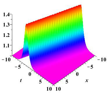
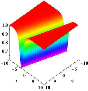
Figure 1. (Color online) The bright and dark solitons of the CLL-NLS with parameters: (a) $a=1.5,c=1$ and $\beta=0.2$, (b) $a=1.5,c=1$ and $\beta=-0.2$.

For $n=2$, let $D=1$, $\lambda_{1}=\alpha_{1}+{\rm i}\beta_{1}$ and $\lambda_{2}=-\alpha_{1}+{\rm i}\beta_{1}$ in theorem 2.2, then

$$r_{2}=\frac{(-\overline{\lambda}_{1}{|f_{1}|}^{2}-\lambda_{1}{|g_{1}|}^{2})r+2{\rm i}(\overline{\lambda}_{1}^{2}-\lambda_{1}^{2})f_{1}\overline{g}_{1}}{-\overline{\lambda}_{1}|g_{1}|^{2}-\lambda_{1}|f_{1}|^{2}}$$ (37)

gives the second-order solution of the CLL-NLS. For convenience, let $a=2\,{\beta_{{1}}}^{2}-\frac{1}{2}\,{c}^{2}-2\,{\alpha_{{1}}}^{2}+1$, then

$$r_{2}=-\frac{K_{1}c\cos\theta_{1}+{\rm i}K_{2}c\sin\theta_{1}+(K_{3}c+K_{5})\cosh\theta_{2}+{\rm i}(K_{6}-K_{4}c)\sinh\theta_{2}}{-K_{1}\cos\theta_{1}+{\rm i}K_{2}\sin\theta_{1}+K_{3}\cosh\theta_{2}+{\rm i}K_{4}\sinh\theta_{2}}\exp(-{\rm i}\rho)$$ (38)

with

$$\theta_{1}= ((4\alpha_{1}^{2}-4\beta_{1}^{2}-2)t-x)K_{0},\quad\theta_{2}=4\alpha_{1}\beta_{1}tK_{0},\quad K_{0}=\sqrt{(c^{2}+4\alpha_{1}^{2})(c^{2}-4\beta_{1}^{2})},$$

$$K_{1}= 8\alpha_{1}^{3}\beta_{1}+2c^{2}\alpha_{1}\beta_{1}+2\alpha_{1}\beta_{1}K_{0},\quad K_{2}=2c^{2}\alpha_{1}\beta_{1}-8\alpha_{1}\beta_{1}^{3}+2\alpha_{1}\beta_{1}K_{0},$$

$$K_{3}= c^{3}\alpha_{1}+4c\alpha_{1}^{3}+c\alpha_{1}K_{0},\quad K_{4}=4c\beta_{1}^{3}-c^{3}\beta_{1}-c\beta_{1}K_{0},$$

$$K_{5}= -8c^{2}\alpha_{1}\beta_{1}^{2}-32\alpha_{1}^{3}\beta_{1}^{2}-8\alpha_{1}\beta_{1}^{2}K_{0},\quad K_{6}=8c^{2}\alpha_{1}^{2}\beta_{1}-32\alpha_{1}^{2}\beta_{1}^{3}+8\alpha_{1}^{2}\beta_{1}K_{0}.$$

Note that the trajectory of $r_{2}$ is defined by

$$(4\alpha_{1}^{2}-4\beta_{1}^{2}-2)t-x=0,$$

if $K_{0}^{2}<0$, and by

$$4\alpha_{1}\beta_{1}t=0,$$

if $K_{0}^{2}>0$. Thus, we can get both the spatial periodic breather solution (similar to the NLS Akhmediev breather [77]) and the temporal periodic breather solution (similar to the NLS Kuznetsov-Ma breather [78, 79]). In fact, this solution $r_{2}$ can travel periodically with an additional velocity in the $(x,t)$-plane. Three kinds of breather solutions, propagating along the $(x,t)$-plane with different angles, are shown in Fig. 2.

$|r_{2}|$   $|r_{2}|$   $|r_{2}|$

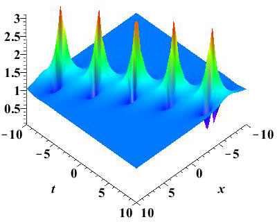
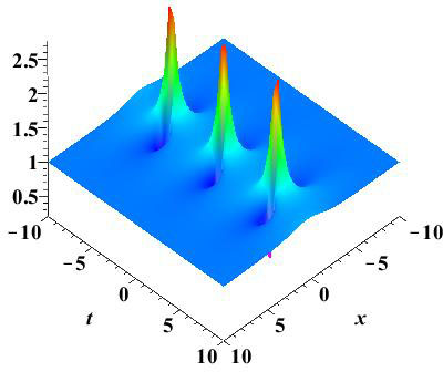
Figure 2. (Color online) The breather solutions of the CLL-NLS with parameters: (a) $c=1$, $\alpha=0.75$ and $\beta=0.4$; (b) $c=1$, $\alpha=0.8$ and $\beta=0.55$; (c) $c=1$, $\alpha_{1}^{2}=\beta_{1}^{2}+\frac{1}{2}$, and $\beta_{1}=0.52$.

After a simple analysis, we emphasize that the periodicity of the breather solution is proportional to $\frac{1}{K_{0}}$, i.e. when $K_{0}$ tends to zero, the distance of two peaks goes to infinity which leaves only one peak locating on the $(x,t)$-plane. Thus, let $c\rightarrow 2\beta_{1}$, then $r_{2}$ in (38) leads to a new solution, having the property to possess only one local peak and surrounding two holes which is very similar to the Peregrine solution and therefore, being an appropriate to model RWs. This kind of doubly-localized rational solution is described by

$$r_{2r}=\frac{2\beta_{1}(L_{11}+{\rm i}L_{12})}{L_{11}+{\rm i}L_{13}+4}\exp(-{\rm i}\rho),$$ (39)

with

$$L_{11}= (16\alpha_{1}^{2}\beta_{1}^{2}+16\beta_{1}^{4})x^{2}-(128\alpha_{1}^{4}\beta_{1}^{2}-64\beta_{1}^{4}-64\alpha_{1}^{2}\beta_{1}^{2}-128\beta_{1}^{6})xt-(256\alpha_{1}^{4}\beta_{1}^{2}-64\alpha_{1}^{2}\beta_{1}^{2}$$

$$-256\beta_{1}^{8}-256\alpha_{1}^{6}\beta_{1}^{2}-256\beta_{1}^{6}-64\beta_{1}^{4})t^{2}-3,$$

$$L_{12}= 8\beta_{1}^{2}x+16\beta_{1}^{2}t-96\alpha_{1}^{2}\beta_{1}^{2}t,\quad L_{13}=(32\alpha_{1}^{2}\beta_{1}^{2}-64\beta_{1}^{4}-16\beta_{1}^{2})t-8\beta_{1}^{2}x.$$

When $x$ and $t$ tend to infinity, $|r_{2r}|$ tends to $2\beta_{1}$. Moreover, the maximum peak amplitude is equal to $6\beta_{1}$, which is three times the background amplitude. The profiles are shown in Fig. 3, and this solution is the same as presented in [64]. The latter has been derived using the Hirota bilinear method, while difficulties using the DT have been also discussed in [64].

4.3. Higher-order rogue wave solutions

Inspired by above method, we consider the higher-order RWs of the CLL-NLS in this subsection. Generally, it is difficult to derive higher-order RWs from multi-breather solutions, since the explicit expression of $n$-th order breather is very challenging to calculate when $n>4$. Similarly for the NLS, for which the formulae is given by theorem 2.2, an indeterminate form $\frac{0}{0}$ is a consequence, when eigenvalues $\lambda_{k}$ tend to a limit point (from a breather to a doubly-localized RW solution). Thus, we derive the higher-order RWs directly from the determinant expressions of solutions in theorem 2.2 by adopting a Taylor expansion [16, 50, 51, 52].

Theorem 4.2.

Let $n=2N$, $\lambda_{2k-1}=\sqrt{\frac{1-a}{2}}+\frac{{\rm i}c}{2}+\epsilon^{2}$ $(a<1)$ and $\lambda_{2k}=-\overline{\lambda}_{2k-1}$, by applying the Taylor expansion, then a determinant expression of the $N$-th order RW is given as

$$r_{nr}=\frac{|\widehat{\Delta}_{n}^{1}|}{|\widehat{\Delta}_{n}^{2}|}r-2{\rm i}\frac{|\widehat{\Delta}_{n}^{4}|}{|\widehat{\Delta}_{n}^{2}|},$$ (40)

where $\widehat{\Delta}_{n}^{k}$ $(k=1,2,3,4)$ are defined by

$$\widehat{\Delta}_{n}^{k}=\left(\left.\frac{\partial^{n_{i}}}{\partial\epsilon^{n_{i}}}\right|_{\epsilon=0}({\Delta}_{n}^{k})_{ij}\right)_{n\times n}.$$ (41)

Here, $n_{i}=i$ if $i$ is odd and $n_{i}=i-1$ if $i$ is even.

Note that $D$ is a constant in (35), it is reasonable to choose $D=\exp({\rm i}\sqrt{S}(\sum^{N-1}_{l=1}s_{l}\epsilon^{2l})$. Here, $D$ goes to $1$ when $\epsilon$ goes to zero. Thus, there exist $N+1$ free parameters ($s_{1},s_{2},\cdots,s_{N-1};a,c$) in an $N$-th order RW solution. Next, we derive RWs with these parameters, and consider their dynamical evolution. For convenience, let $a=-1$ and $c=1$ in the following context.

For $N=2$, the second-order RW of the CLL-NLS is

$$r_{4r}=\frac{L_{21}}{L_{22}}\exp(-{\rm i}\rho),$$ (42)

where

$$L_{21}= 125\,{x}^{6}+150\,{\rm i}{x}^{5}-750\,t{x}^{5}-285\,{x}^{4}+3375\,{t}^{2}{x}^{4}-2100\,{\rm i}{x}^{4}t-156\,{\rm i}{x}^{3}-8500\,{t}^{3}{x}^{3}$$

$$+2220\,t{x}^{3}+8100\,{\rm i}{t}^{2}{x}^{3}-24000\,{\rm i}{t}^{3}{x}^{2}-14850\,{t}^{2}{x}^{2}-333\,{x}^{2}+16875\,{t}^{4}{x}^{2}+2160\,{\rm i}t{x}^{2}$$

$$-270\,tx-18750\,{t}^{5}x+33750\,{\rm i}{t}^{4}x+28500\,{t}^{3}x-8100\,{\rm i}x{t}^{2}-90\,{\rm i}x+45+15625\,{t}^{6}$$

$$+1044\,{\rm i}t+600\,{\rm i}{t}^{3}-2205\,{t}^{2}-37500\,{\rm i}{t}^{5}-26625\,{t}^{4}+(-300\,{x}^{3}-1800\,{\rm i}{x}^{2}+4500\,t{x}^{2}$$

$$+1800\,{\rm i}tx+180\,x-4500\,{t}^{2}x-4500\,{t}^{3}-432\,{\rm i}+540\,t+7200\,{\rm i}{t}^{2})s_{1},$$

$$L_{22}= -125\,{x}^{6}+750\,t{x}^{5}+150\,{\rm i}{x}^{5}-15\,{x}^{4}-3375\,{t}^{2}{x}^{4}-600\,{\rm i}{x}^{4}t+180\,t{x}^{3}+8500\,{t}^{3}{x}^{3}$$

$$+84\,{\rm i}{x}^{3}+2100\,{\rm i}{t}^{2}{x}^{3}+2250\,{t}^{2}{x}^{2}-3000\,{\rm i}{t}^{3}{x}^{2}-16875\,{t}^{4}{x}^{2}-171\,{x}^{2}-360\,{\rm i}{x}^{2}t$$

$$-4500\,{t}^{3}x+18750\,{t}^{5}x-900\,{\rm i}x{t}^{2}+3750\,{\rm i}{t}^{4}x+270\,tx+54\,{\rm i}x-15625\,{t}^{6}+144\,{\rm i}t$$

$$+3600\,{\rm i}{t}^{3}-3195\,{t}^{2}-10875\,{t}^{4}-9+(300\,{x}^{3}-4500\,t{x}^{2}+4500\,{t}^{2}x-180\,x+1800\,{\rm i}tx$$

$$+4500\,{t}^{3}-1800\,{\rm i}{t}^{2}-72\,{\rm i}+3060\,t)s_{1},$$

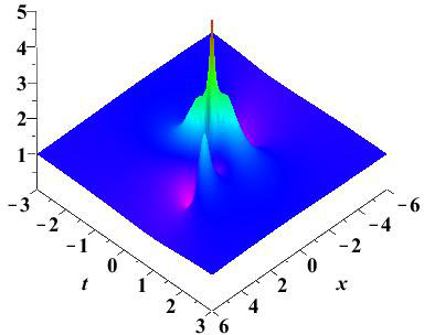
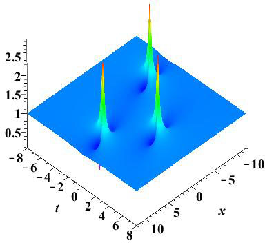
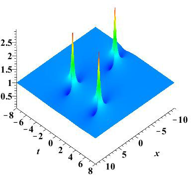
Figure 4. (Color online) The second-order RW of the CLL-NLS with parameters: (a) $s_{1}=0$; (b) $s_{1}=100-100{\rm i}$; (c) $s_{1}=100+100{\rm i}$.

where $s_{1}$ is a free complex parameter. The maximum amplitude of $|r_{4r}|$ is equal to $5$ when $s_{1}=0$, which is reached at $(x=0,\,t=0)$. This solution is shown in Fig. 4(a). Allocating different values to $s_{1}$, we can obtain RWs which are distinct from the above one. For example, RWs with $s_{1}=100-100{\rm i}$ and $s_{1}=100+100{\rm i}$ are shown in Fig. 4(b) and Fig. 4(c), respectively. Both of them possess three intensity peaks, located at different time and space values. Each peak is similar to a first-order RW, shown in Fig. 3(a). Moreover, solution $r_{4r}$ in Fig. 4(b) is different from the one in Fig. 4(c), since three peaks in each solution are arrayed in different directions.

For $N=3$, according to theorem 4.2, we can obtain the third-order RW solution of the CLL-NLS equation. However, its expression, with two non-zero parameters $s_{1}$ and $s_{2}$, is very cumbersome, that we just provide the exact expression in the case $s_{1}=s_{2}=0$, i.e.

$$r_{6r}=\frac{L_{31}}{L_{32}}\exp(-{\rm i}\rho),$$ (43)

with

$$L_{31}= -3125\,{x}^{12}+37500\,t{x}^{11}-7500\,{\rm i}{x}^{11}-281250\,{t}^{2}{x}^{10}+150000\,{\rm i}t{x}^{10}+18750\,{x}^{10}+1437500\,{t}^{3}{x}^{9}$$

$$-1237500\,{\rm i}{t}^{2}{x}^{9}+22500\,{\rm i}{x}^{9}-322500\,t{x}^{9}+3386250\,{t}^{2}{x}^{8}+6975000\,{\rm i}{t}^{3}{x}^{8}-5671875\,{t}^{4}{x}^{8}$$

$$-495000\,{\rm i}t{x}^{8}+31725\,{x}^{8}+5130000\,{\rm i}{t}^{2}{x}^{7}+63720\,{\rm i}{x}^{7}+17475000\,{t}^{5}{x}^{7}+84600\,t{x}^{7}$$

$$-19890000\,{t}^{3}{x}^{7}-27975000\,{\rm i}{t}^{4}{x}^{7}+87240000\,{\rm i}{t}^{5}{x}^{6}+82807500\,{t}^{4}{x}^{6}+116676\,{x}^{6}-858240\,{\rm i}t{x}^{6}$$

$$-33000000\,{\rm i}{t}^{3}{x}^{6}-3338100\,{t}^{2}{x}^{6}-43637500\,{t}^{6}{x}^{6}+2230200\,{\rm i}{t}^{2}{x}^{5}+87375000\,{t}^{7}{x}^{5}$$

$$+26829000\,{t}^{3}{x}^{5}+31320\,t{x}^{5}+133155000\,{\rm i}{t}^{4}{x}^{5}-209775000\,{\rm i}{t}^{6}{x}^{5}-245835000\,{t}^{5}{x}^{5}+129384\,{\rm i}{x}^{5}$$

$$+401250000\,{\rm i}{t}^{7}{x}^{4}+550312500\,{t}^{6}{x}^{4}-146475\,{x}^{4}-1717200\,{\rm i}t{x}^{4}-366750000\,{\rm i}{t}^{5}{x}^{4}$$

$$-93881250\,{t}^{4}{x}^{4}-607500\,{t}^{2}{x}^{4}-141796875\,{t}^{8}{x}^{4}-3330000\,{\rm i}{t}^{3}{x}^{4}+1315980\,t{x}^{3}$$

$$-52380\,{\rm i}{x}^{3}-585937500\,{\rm i}{t}^{8}{x}^{3}+696450000\,{\rm i}{t}^{6}{x}^{3}+4222800\,{\rm i}{t}^{2}{x}^{3}+6975000\,{\rm i}{t}^{4}{x}^{3}$$

$$+179687500\,{t}^{9}{x}^{3}-902250000\,{t}^{7}{x}^{3}+209925000\,{t}^{5}{x}^{3}+9702000\,{t}^{3}{x}^{3}-846000000\,{\rm i}{t}^{7}{x}^{2}$$

$$-12429450\,{t}^{2}{x}^{2}-175781250\,{t}^{10}{x}^{2}+656250000\,{\rm i}{t}^{9}{x}^{2}+1078593750\,{t}^{8}{x}^{2}-19872000\,{\rm i}{t}^{3}{x}^{2}$$

$$+126900000\,{\rm i}{t}^{5}{x}^{2}-332212500\,{t}^{6}{x}^{2}+17347500\,{t}^{4}{x}^{2}-62370\,{x}^{2}+887760\,{\rm i}t{x}^{2}$$

$$+117187500\,{t}^{11}x-11340\,{\rm i}x+25825500\,{t}^{3}x-299475000\,{\rm i}{t}^{6}x-286740\,tx+52245000\,{\rm i}{t}^{4}x$$

$$+621562500\,{\rm i}{t}^{8}x-5046300\,{\rm i}x{t}^{2}-492187500\,{\rm i}{t}^{10}x+313875000\,{t}^{7}x-128925000\,{t}^{5}x$$

$$-839062500\,{t}^{9}x-190350000\,{\rm i}{t}^{5}-46875000\,{\rm i}{t}^{9}-715230\,{t}^{2}-48828125\,{t}^{12}+2835$$

$$-5761800\,{\rm i}{t}^{3}+222328125\,{t}^{8}-47833875\,{t}^{4}+53550000\,{\rm i}{t}^{7}+234375000\,{\rm i}{t}^{11}+363281250\,{t}^{10}$$

$$+291937500\,{t}^{6}+158760\,{\rm i}t,$$

$$L_{32}= -3125\,{x}^{12}+37500\,t{x}^{11}+7500\,{\rm i}{x}^{11}-75000\,{\rm i}t{x}^{10}+3750\,{x}^{10}-281250\,{t}^{2}{x}^{10}+487500\,{\rm i}{t}^{2}{x}^{9}$$

$$+7500\,{\rm i}{x}^{9}+1437500\,{t}^{3}{x}^{9}-22500\,t{x}^{9}-5671875\,{t}^{4}{x}^{8}-13275\,{x}^{8}-90000\,{\rm i}t{x}^{8}+461250\,{t}^{2}{x}^{8}$$

$$-2100000\,{\rm i}{t}^{3}{x}^{8}-3090000\,{t}^{3}{x}^{7}+6975000\,{\rm i}{t}^{4}{x}^{7}+84600\,t{x}^{7}+37080\,{\rm i}{x}^{7}+17475000\,{t}^{5}{x}^{7}$$

$$-90000\,{\rm i}{t}^{2}{x}^{7}-998100\,{t}^{2}{x}^{6}-43637500\,{t}^{6}{x}^{6}+13057500\,{t}^{4}{x}^{6}-17490000\,{\rm i}{t}^{5}{x}^{6}-239760\,{\rm i}t{x}^{6}$$

$$+2100000\,{\rm i}{t}^{3}{x}^{6}-81324\,{x}^{6}+34875000\,{\rm i}{t}^{6}{x}^{5}+4509000\,{t}^{3}{x}^{5}+97848\,{\rm i}{x}^{5}-35955000\,{t}^{5}{x}^{5}$$

$$+489240\,t{x}^{5}+1290600\,{\rm i}{t}^{2}{x}^{5}+87375000\,{t}^{7}{x}^{5}-10215000\,{\rm i}{t}^{4}{x}^{5}-3469500\,{t}^{2}{x}^{4}+11205\,{x}^{4}$$

$$+28800000\,{\rm i}{t}^{5}{x}^{4}-7031250\,{t}^{4}{x}^{4}-52500000\,{\rm i}{t}^{7}{x}^{4}+62062500\,{t}^{6}{x}^{4}-141796875\,{t}^{8}{x}^{4}$$

$$-3780000\,{\rm i}{t}^{3}{x}^{4}-216000\,{\rm i}t{x}^{4}-48450000\,{\rm i}{t}^{6}{x}^{3}+961200\,{\rm i}{t}^{2}{x}^{3}+106380\,t{x}^{3}+26460\,{\rm i}{x}^{3}$$

$$+60937500\,{\rm i}{t}^{8}{x}^{3}-3375000\,{\rm i}{t}^{4}{x}^{3}+1125000\,{t}^{5}{x}^{3}-62250000\,{t}^{7}{x}^{3}+9702000\,{t}^{3}{x}^{3}+179687500\,{t}^{9}{x}^{3}$$

$$+5724000\,{\rm i}{t}^{3}{x}^{2}-73102500\,{t}^{4}{x}^{2}-87480\,{\rm i}t{x}^{2}-46875000\,{\rm i}{t}^{9}{x}^{2}-158512500\,{t}^{6}{x}^{2}+67500000\,{\rm i}{t}^{7}{x}^{2}$$

$$-20250\,{x}^{2}+1891350\,{t}^{2}{x}^{2}-175781250\,{t}^{10}{x}^{2}-18281250\,{t}^{8}{x}^{2}+66150000\,{\rm i}{t}^{5}{x}^{2}+4860\,{\rm i}x$$

$$+11340\,tx+23437500\,{\rm i}{t}^{10}x+98437500\,{t}^{9}x-45225000\,{\rm i}{t}^{6}x-882900\,{\rm i}{t}^{2}x-526500\,{t}^{3}x$$

$$+146475000\,{t}^{5}x+13095000\,{\rm i}{t}^{4}x+117187500\,{t}^{11}x-47812500\,{\rm i}{t}^{8}x+331875000\,{t}^{7}x$$

$$-345796875\,{t}^{8}-109912500\,{t}^{6}-405-8100000\,{\rm i}{t}^{5}+32400\,{\rm i}t-48828125\,{t}^{12}-990630\,{t}^{2}$$

$$-24883875\,{t}^{4}+56250000\,{\rm i}{t}^{9}-152343750\,{t}^{10}+52200000\,{\rm i}{t}^{7}+4276800\,{\rm i}{t}^{3}.$$

$|r_{2r}|$   $|r_{2r}|$

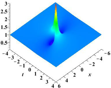
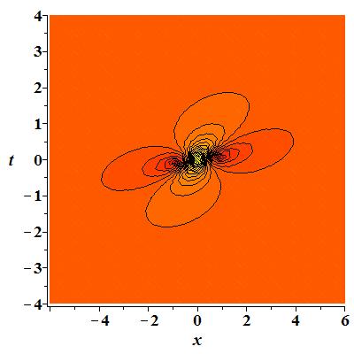
Figure 3. (Color online) The first-order RW solution of the CLL-NLS with parameters: $\alpha_{1}=-1,\,\beta_{1}=0.5$. The right panel is the density plot of the left.

$|r_{4r}|$   $|r_{4r}|$   $|r_{4r}|$

The maximum amplitude is equal to $7$ which occurs at $(0,\,0)$, its profile is shown in Fig. 5(a). Let $s_{1}\neq 0$ and $s_{2}\neq 0$, we obtain other solutions which are different from the one given in Fig. 5(a). In each of these solutions, the third-order RW is split into six intensity peaks which are similar to a first-order RW. These six peaks, located at different point of time and space, make up different profiles. As example, three such solutions are displayed in Fig. 5(b-d) with $(s_{1},\,s_{2})=(100,\,0)$, $(s_{1},\,s_{2})=(0,\,5000)$, and $(s_{1},\,s_{2})=(100,\,13000)$, respectively. In Fig. 5(b), these six intensity form a triangle. In Fig. 5(c), they compose a pentagon with five peaks locating on the shell and the other one locating on the center. In Fig. 5(d), three peaks compose a triangle and the other three peaks compose a part of a circular arc.

$|r_{6r}|$   $|r_{6r}|$
$|r_{6r}|$   $|r_{6r}|$

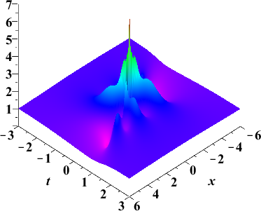
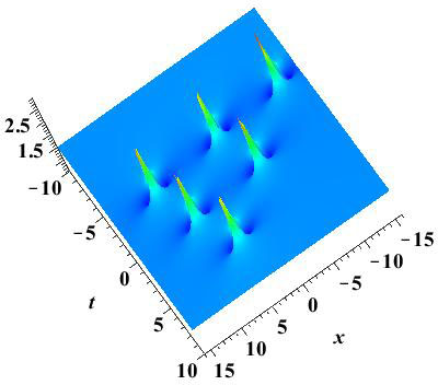
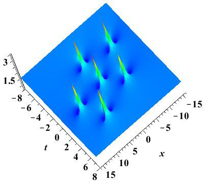
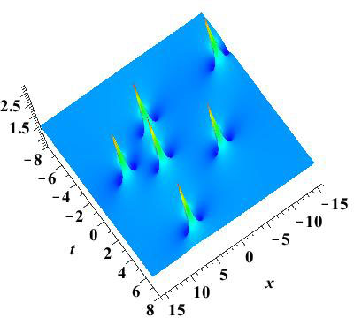
Figure 5. (Color online) The third-order RW of the CLL-NLS with parameters $(s_{1},\,s_{2})$ as: (a) $(0,0)$; (b) $(100,0)$; (c) $(0,5000)$; (d) $(100,13000)$.

Let $N=4$ in theorem 4.2, then $r_{8r}$ gives a fourth-order RW of the CLL-NLS with three parameters $s_{1},\,s_{2}$ and $s_{3}$. Let $(s_{1},\,s_{2},\,s_{3})=(0,\,0,\,0)$, $r_{8r}$ leads to a solution with a highest peak surrounded by several gradually decreasing peaks in two sides along $t$-direction, which is the fundamental pattern and is shown in Fig 6(a). The amplitude of this solution is $9$ located at the origin of coordinate. Furthermore, allocating different values to $(s_{1},\,s_{2},\,s_{3})$, we obtain a hierarchy of solutions, which have a triangle pattern, a pentagon pattern, a circular pattern with a inner second-order fundamental pattern or triangle pattern. These solutions are shown in Fig. 6(b-c) and Fig. 7.

$|r_{8r}|$   $|r_{8r}|$   $|r_{8r}|$

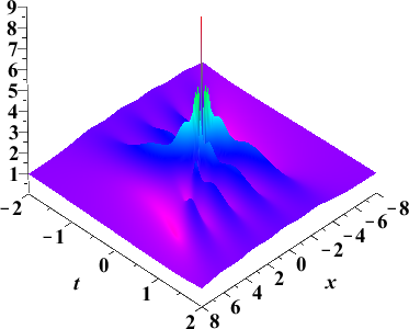
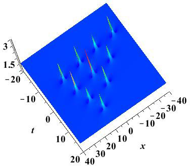
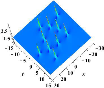
Figure 6. (Color online) The fourth-order RW of the CLL-NLS with parameters $(s_{1},\,s_{2},\,s_{3})$ as: (a) $(0,0,0)$; (b) $(500,0,0)$; (c) $(0,50000,0)$.

$|r_{8r}|$   $|r_{8r}|$

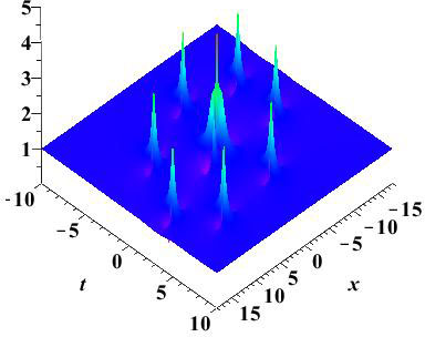
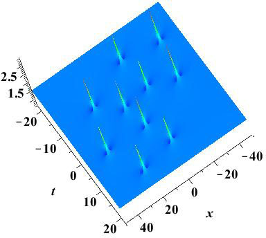
Figure 7. (Color online) The fourth-order RW in circular pattern of the CLL-NLS with parameters $(s_{1},\,s_{2},\,s_{3})$ as: (a) $(0,0,500000)$; (b) $(500,0,50000000)$.

All the results are derived as a consequence of theorem 4.2 and can be trivially extended to the higher-order RWs. That is, the explicit expressions of other higher-order solutions can be obtained in a straightforward manner. However, we will omit this, since expressions are too cumbersome to be explicitly written here. All solutions, presented above, have been verified analytically by symbolic computation through a Maple computer software.

5. Localization characters of CLL-NLS rogue waves

In this section, we consider the localization characters of the RW of the CLL-NLS as well as the influence of SSE on these localization. First, we need to define the length and width of the RW solution as described in [59]. In order to compare the latter properties with localization of NLS RWs [16, 59], we replace the parameters $\alpha_{1}$ and $\beta_{1}$ with $a$ and $c$ in (39). That is, we substitute $\alpha_{1}=\sqrt{\frac{1-a}{2}}$ $(a<1)$ and $\beta_{1}=\frac{c}{2}$ into (39). In this case, the first-order RW of the CLL-NLS is expressed as the following

$$r_{2r}=\frac{L_{n}}{L_{d}}c\exp(-{\rm i}\rho),$$ (44)

with

$$L_{n}= 3-{c}^{4}{x}^{2}-4\,{t}^{2}{c}^{4}-4\,{c}^{6}{t}^{2}-{c}^{8}{t}^{2}-2\,{c}^{6}xt+8\,{\rm i}t{c}^{2}-12\,{\rm i}{c}^{2}ta-4\,{c}^{4}xt+8\,{c}^{2}{t}^{2}{a}^{3}-2\,{c}^{2}{x}^{2}$$

$$+2\,a{c}^{2}{x}^{2}-8\,{c}^{2}xta-2\,{\rm i}{c}^{2}x-8\,{c}^{2}{t}^{2}{a}^{2}+8\,{c}^{2}xt{a}^{2},$$

$$L_{d}= -1-{c}^{4}{x}^{2}-4\,{t}^{2}{c}^{4}-4\,{c}^{6}{t}^{2}-{c}^{8}{t}^{2}-2\,{c}^{6}xt+4\,{\rm i}{c}^{2}ta+4\,{\rm i}{c}^{4}t-4\,{c}^{4}xt+8\,{c}^{2}{t}^{2}{a}^{3}-2\,{c}^{2}{x}^{2}$$

$$+2\,a{c}^{2}{x}^{2}-8\,{c}^{2}xta+2\,{\rm i}{c}^{2}x-8\,{c}^{2}{t}^{2}{a}^{2}+8\,{c}^{2}xt{a}^{2}.$$

As it is known, there exist two holes near the peak in the first-order RW. These two holes are located at $P_{1}=({\frac{-18a+12}{\sqrt{-24\,a+24+3\,{c}^{2}}\left(2\,a-2-{c}^{2}\right)c}},\,{\frac{3}{\sqrt{-24\,a+24+3\,{c}^{2}}\left(2\,a-2-{c}^{2}\right)c}})$ and $P_{2}=({\frac{18a-12}{\sqrt{-24\,a+24+3\,{c}^{2}}\left(2\,a-2-{c}^{2}\right)c}},$ $\,{\frac{-3}{\sqrt{-24\,a+24+3\,{c}^{2}}\left(2\,a-2-{c}^{2}\right)c}})$. It is obvious that $P_{1}$ and $P_{2}$ are on the line $l_{1}:\,x=-2(3a-2)t$. On the background plane with height $|r_{2r}|=c$, the contour line is a hyperbola

$$\left(4\,{c}^{6}-4\,{c}^{4}-8\,{c}^{2}{a}^{3}+3\,{c}^{8}+24\,a{c}^{4}-16\,{a}^{2}{c}^{4}+8\,{c}^{2}{a}^{2}+4\,a{c}^{6}\right){t}^{2}+\left(-4\,a{c}^{4}+4\,{c}^{6}+8\,{c}^{4}+8\,{c}^{2}a\right.$$

$$\left.-8\,{c}^{2}{a}^{2}\right)xt-1+\left({c}^{4}+2\,{c}^{2}-2\,{c}^{2}a\right){x}^{2}=0,$$ (45)

which intersects with the line $l_{1}$ at two points $P_{3}=({\frac{6a-4}{\sqrt{-8\,a+3\,{c}^{2}+8}\left(2\,a-2-{c}^{2}\right)c}},\,-{\frac{1}{\sqrt{-8\,a+3\,{c}^{2}+8}\left(2\,a-2-{c}^{2}\right)c}})$ and $P_{4}=({-\frac{6a-4}{\sqrt{-8\,a+3\,{c}^{2}+8}\left(2\,a-2-{c}^{2}\right)c}},\,{\frac{1}{\sqrt{-8\,a+3\,{c}^{2}+8}\left(2\,a-2-{c}^{2}\right)c}})$. We define the tangential direction of hyperbola to be at two points $P_{3}$ and $P_{4}$, which is the length-direction, as described by a line $l_{2}$ : $x=-(2a+3/2c^{2})t$. The density plot for $|r_{2r}|^{2}$ combined with the hyperbola and the length-direction is displayed in Fig. 8.

(a)   (b)

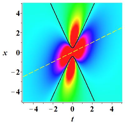
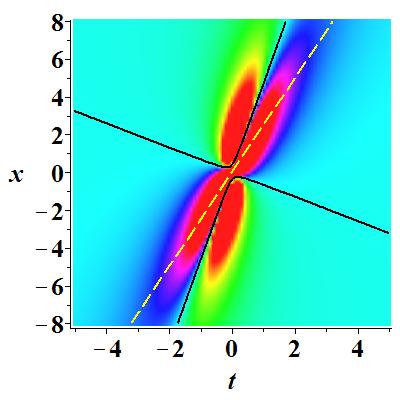
Figure 8. (Color online) The density plots of the first-order RW $|r_{2r}|^{2}$ with hyperbola($|r_{2r}|^{2}=c^{2}$) and length-direction. (a) $a=-1,\,c=1$. (b) $a=-2,\,c=1$. The black solid line is hyperbola, the yellow dash line is the length-direction.

Since the contour line is not closed on the background in the length-direction, we have to select a contour $|r_{2r}|^{2}-2c^{2}=0$ with height twice the background such that it is closed. The closed contour is useful to discuss the localization characters of the the first-order RW. It intersects with the length-direction at two points. We define the distance $d^{L}$ of these two points as the length of the first-order RW, and we determine the projection $d^{W}$ of $|P_{1}P_{2}|$ on the width-direction, which is perpendicular to the length-direction, to be the width of the first-order RW. Through a simple calculation, we obtain

$$d^{L}=\frac{{d^{L}}_{n}}{{d^{L}}_{d}},$$ (46)

with

$${d^{L}}_{n}= 2\,\sqrt{\left(4+16\,{a}^{2}+24\,{c}^{2}a+9\,{c}^{4}\right)\left(48+9\,{c}^{4}+48\,{a}^{2}+46\,{c}^{2}-96\,a-46\,{c}^{2}a+2\,\sqrt{M_{{1}}}\right)},$$

$${d^{L}}_{d}= (8\,a-8-{c}^{2})(2\,a-2-{c}^{2})c^{2},$$

$$M_{1}= 1024-4096\,a+22\,{c}^{8}-4992\,{c}^{2}a+1024\,{a}^{4}+242\,{c}^{6}-4096\,{a}^{3}-1664\,{c}^{2}{a}^{3}-242\,a{c}^{6}$$

$$+976\,{a}^{2}{c}^{4}-1952\,a{c}^{4}+4992\,{c}^{2}{a}^{2}+1664\,{c}^{2}+6144\,{a}^{2}+976\,{c}^{4},$$

and

$$d^{W}=\frac{{d^{W}}_{n}}{{d^{W}}_{d}},$$ (47)

while

$${d^{W}}_{n}=6(8a-3c^{2}-8),\quad{d^{W}}_{d}=\sqrt{\left(-24a+24+3c^{2}\right)\left(4+16a^{2}+24c^{2}+9c^{4}\right)}\left(2a-2-c^{2}\right)c.$$

The length $d^{L}$ and width $d^{W}$ are related to $a$ and $c$, and their profiles are plotted in Fig. 9.

(a)   (b)

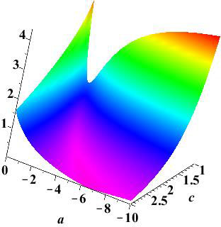
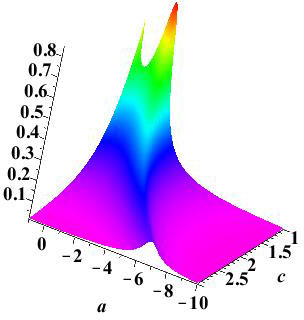
Figure 9. (Color online) The localization characters of the first-order RW of the CLL-NLS, which are two functions of $a$ and $c$. (a) The length $d^{L}$. (b)The width $d^{W}$.

If one fixes the parameter $c$, the length decreases with the increase of $a$ at first and then increases until $a=1$. On the other hand, the width increases first, decreases, and then increases again until $a=1$. For example, when $c=1$, the length decreases with $a$ if $a\in(-\infty,-0.88)$ and increases with $a$ if $a\in(-0.88,1)$. At the same time, the width increases with $a$ if $a\in(-\infty,-0.69)$ or $a\in(0.52,1)$ and decreases with $a$ if $a\in(-0.69,0.52)$. Furthermore, when $a$ tends to $-\infty$, $d^{L}$ tends to $2\sqrt{7}$ and $d^{W}$ tends to $0$, $d^{L}$ reaches to the minimum $1.32$ when $a=-0.88$ and gets to the maximum $62.42$ when $a\rightarrow 1$, and $d^{W}$ reaches to the maximum $1.70$ when $a=-0.69$. In order to provide a visual support of above analysis on the trend with respect to $a$ of two localization characters of the RW for the CLL-NLS, two curves for $d^{L}$ and $d^{W}$ with fixed $c=1$ are given in Fig. 10(a).

In order to consider the contribution of the SSE on the localization characters of the RW, we define the length and width of the RW as mentioned above for the NLS ${\rm i}r_{t}+r_{xx}+|r|^{2}r=0$, which is trivially given by ignoring the SSE term in the CLL-NLS. After applying a scaling transformation, due to the the different coefficient of nonlinear term, the first-order RW of the NLS can be obtained from the results, reported in [16]. Then, the length and width of the first-order RW of the NLS are expressed by

$${d^{L}}_{NLS}=\frac{\sqrt{7(1+4a^{2})}}{2c^{2}},\qquad{d^{W}}_{NLS}=\frac{\sqrt{3}}{(1+4a^{2})c},$$ (48)

and the length direction is described by a line $l_{2NLS}$: $x=2at$.

Set $c=1$, then ${d^{L}}_{NLS}$ and ${d^{W}}_{NLS}$ reach the minimum $\frac{\sqrt{7}}{2}$ and the maximum $\sqrt{3}$ at $a=0$, respectively. It implies that the maximum of width and the minimum of length of the RW for the NLS are roughly equal to the corresponding values of the RW for the CLL-NLS. The width of the RW for the NLS also tends to $0$ when $a\rightarrow\pm\infty$. However, the length tends to $+\infty$, when $a\rightarrow\pm\infty$. There is no oscillation interval for the width of the RW solution of the NLS. This is different from the analogous CLL-NLS. The profiles of ${d^{L}}_{NLS}$ and ${d^{W}}_{NLS}$ with $c=1$ are given in Fig. 10(b).

(a)   (b)

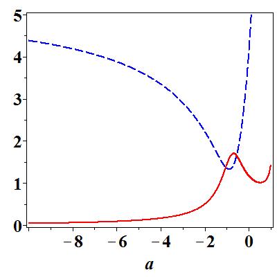
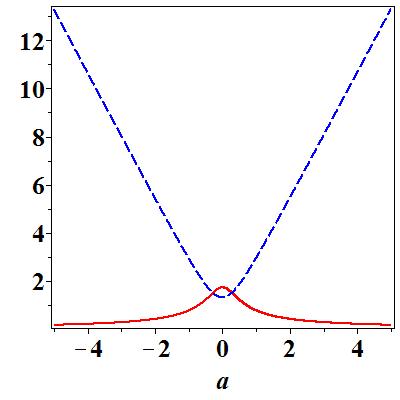
Figure 10. (Color online) The length $d^{L}$ and the width $d^{W}$ for the first-order RW with c=1. The blue dash line indicates the length, and the red solid line denotes the width. (a) The CLL-NLS. (b) The NLS.

Furthermore, we notice that $d^{L}<{d^{L}}_{NLS}$ if $a\in(-\infty,\,-0.47)$ and $d^{L}>{d^{L}}_{NLS}$ if $a\in(-0.47,1)$, $d^{W}<{d^{W}}_{NLS}$, if $a\in(-\infty,\,-2.53)$ or $a\in(-0.33,\,0.67)$, and $d^{W}>{d^{W}}_{NLS}$ if $a\in(-2.53,\,-0.33)$ or $a\in(0.67,\,1)$ in the case of $c=1$. These detailed comparisons on localization characters of the first-order RWs are given in table 1 and Fig.11.

(a)   (b)

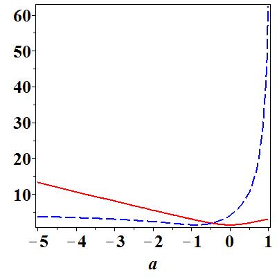
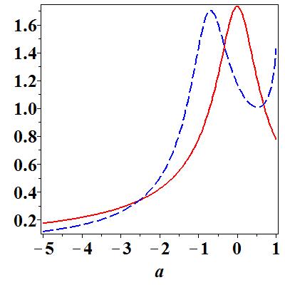
Figure 11. (Color online) The comparison between length (a) and width (b) of the first-order RWs for the NLS equation(red,solid) and the CLL-NLS(blue, dash) with $a<1$ and $c=1$. The left panel has one intersection point ($-0.47,1.82$). There are three intersection points in the right panel: ($-2.53,0.34$), ($-0.33,1.45$),($0.67,1.03$).

This analysis is visually verified by contours of $|r|^{2}$ for heights, being twice higher than the background in Fig.12. Furthermore, since the length and the width of the first-order RW of CLL-NLS are smaller than the corresponding NLS case when $a<-2.53$, respectively, the latter is therefore better than the corresponding NLS one. From an experimental point of view, having a smaller localization, we emphasize therefore a simpler set-up, since the proapgating distance of first-order CLL-NLS RW is considerably smaller compared to the NLS case. The opposite case is valid for $-0.47<a<-0.33$ and $0.67<a<1$, where the CLL-NLS RW is worse. Unfortunately, we have not been able to compare the localization properties, when $a$ belongs to one of the other two intervals, shown in the third and fifth column of table $1$. This is due to the fact that the width and length of the corresponding localization is alternatively smaller or bigger for the CLL-NLS compared to the NLS. In other words, the SSE in the CLL-NLS gives a remarkable change of the localization properties of the first-order RW, although we are not able to claim, if the RW localization for this equation is rather improved or destroyed by this term at different points $(a,c)$, in the parameter space. This is the first impact of the SSE on RW solutions of the CLL-NLS. As second impact we emphasize is that the SSE induces a strong rotation of the direction length on the RW of the CLL-NLS by comparing the two lines $l_{2}$ and $l_{2NLS}$. These two impacts are demonstrated intuitively by contours at a height $2c^{2}$ of the modulus square for the first-order RWs of the CLL-NLS and of the NLS in Fig. 12.

(a)   (b)
(c) (d) (e)

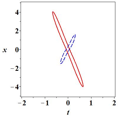
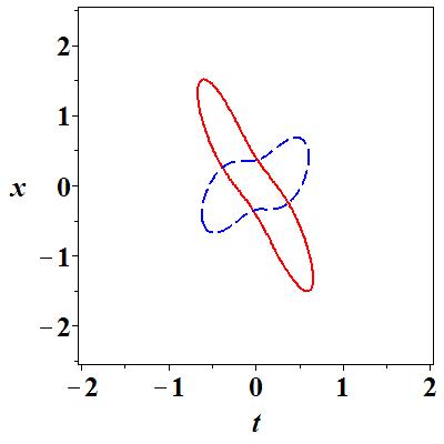
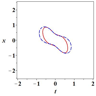
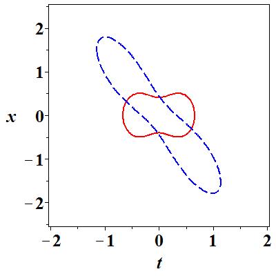
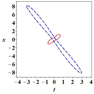
Figure 12. (Color online) The contours of first-order RWs at height($2c^{2}$) twice background with $c=1$ and different values of $a$. The red solid line indicates the NLS and the blue dash line denotes the CLL-NLS. (a) $a=-3$, (b) $a=-1$, (c)$a=-0.4$, (d)$a=0$, (e)$a=0.7$.

The localization characters for the RW in the NLS and CLL-NLS

Values of $a$	$a<-2.53$	$-2.53<a<-0.47$	$-0.47<a<-0.33$	$0.33<a<0.67$	$0.67<a<1$
Length	$d^{L}_{NLS}>d^{L}$	$d^{L}_{NLS}>d^{L}$	$d^{L}_{NLS}<d^{L}$	$d^{L}_{NLS}<d^{L}$	$d^{L}_{NLS}<d^{L}$
Width	$d^{W}_{NLS}>d^{W}$	$d^{W}_{NLS}<d^{W}$	$d^{W}_{NLS}<d^{W}$	$d^{W}_{NLS}>d^{W}$	$d^{W}_{NLS}{}{<}d^{W}$
Localization	NLS$<$CLL-NLS	Indeterminate	NLS$>$CLL-NLS	Indeterminate	NLS$>$CLL-NLS

Table 1. NLS$<$CLL-NLS means the localization of RW in the CLL-NLS is better than NLS, since the width and length of the CLL-NLS RW is smaller compared to the NLS, respectively. NLS$>$CLL-NLS is the opposite case.

6. Conclusions

We have shown that exact fundamental and higher-order solution of the CLL-NLS can be constructed, using the DT. These solutions may describe the accurate propagation of localized structures in nonlinear dispersive media, since dispersion, nonlinearity and SSE have been taken into account. In particular, we provide exact analytical expressions for doubly-localized RW solutions. Furthermore, we discuss the influence of the SSE on the localization characteristics of NLS RWs using visualization contour method. This work may motivate similar studies for higher-order evolution equation of this kind, such for higher-order generalized nonlinear Schrödinger-type equations. In particular, experiments in several nonlinear dispersive media, such in nonlinear optical fibers or in water wave flumes may be a consequence of these studies.

Acknowledgments This work is supported by the NSF of China under Grant No.11271210, the K. C. Wong Magna Fund in Ningbo University. J. S. H acknowledges sincerely Prof. A. S. Fokas for arranging the visit to Cambridge University in 2012-2014 and for many useful discussions. A. C. acknowledges support from the Isaac Newton Institute for Mathematical Sciences.

References

- [1] Benney D.J. and Newell A.C., Nonlinear wave envelopes. J. Math. Phys. 46(1967): 133–139.
- [2] Zakharov V.E., Stability of periodic waves of finite amplitude on the surface of a deep fluid. J. Appl. Mech. Tech. Phys. 9(1968): 190–194.
- [3] Hasegawa A. and Tappert F., Transmission of stationary nonlinear optical pulses in dispersive dielectric fibers. Appl. Phys. Lett. 23(1973): 142–144.
- [4] Ablowitz M.J., Kaup D.J., Newell A.C. and Segur H., Nonlinear-evolution on equations of physical significance. Phys. Rev. Lett. 31(1973): 125–127.
- [5] Peregrine D.H., Water waves, nonlinear Schrödinger equations and their solutions. J. Austral. Math. Soc. Ser. B 25(1983): 16–43.
- [6] Akhmediev N., Eleonskii V. M. and Kulagin N. E., Generation of a periodic sequence of picosecond pulses in an optical fibre: exact solutions. Sov. Phys. JETP 62(1985): 894–899.
- [7] Onorato M., Residori S., Bortolozzo U., Montina A. and Arecci F. T., Rogue waves and their generating mechanisms in different physical contexts. Phys. Rep., 528 (2013), 47–89.
- [8] Akhmediev N., Ankiewicz A. and Soto-Crespo J.M., Rogue waves and rational solutions of the nonlinear Schrödinger equation. Phys. Rev. E 80(2009): 026601.
- [9] Dubard P., Gaillard P., Klein C. and Matveev V.B., On multi-rogue wave solutions of the NLS and positon solutions of the KdV equation. Eur. Phys. J. Spec. Top. 185(2010): 247–258.
- [10] Dubard P. and Matveev V.B., Multi-rogue waves solutions to the focusing NLS and the KP-I equation. Nat. Hazards Earth. Syst. Sci. 11(2011): 667–672.
- [11] Gaillard P., Families of quasi-rational solutions of the NLS and multi-rogue waves. J. Phys. A Math. Theor. 44(2011): 435204.
- [12] Ankiewicz A., Kedziora D.J. and Akhmediev N., Rogue wave triplets. Phys. Lett. A 375(2011): 2782–2785.
- [13] Kedziora D.J., Ankiewicz A. and Akhmediev N., Circular rogue wave clusters. Phys. Rev. E 84(2011): 056611.
- [14] Ohta Y. and Yang J.K., General high-order rogue waves and their dynamics in the nonlinear Schrödinger equation. Proc. R. Soc. A Mathematical, Physical and Engineering Science 468(2012): 1716–1740.
- [15] Guo B.L., Ling L.M. and Liu Q.P., Nonlinear Schrödinger equation: Generalized Darboux transformation and rogue wave solutions. Phys. Rev. E 85(2012): 026607.
- [16] He J.S., Zhang H.R., Wang L.H., Porsezian K. and Fokas A.S., Generating mechanism for higher-order rogue waves. Phys. Rev. E 87(2013): 052914.
- [17] V. I. Shrira and V. V. Geogjaev, What makes the Peregrine soliton so special as a prototype of freak waves?, Journal of Engineering Mathematics 67(2010): 11-22.
- [18] J. M. Dudley, F. Dias, M. Erkintalo and G. Genty, Instabilities, breathers and rogue waves in optics, Nature Photonics 8(2014): 755-7664.
- [19] Akhmediev, N., Ankiewicz, A. and Taki, M., Waves that appear from nowhere and disappear without a trace. Phys. Lett. A 373(2009): 675–678
- [20] Zakharov V. E. and Gelash A. A., Nonlinear stage of modulation instability. Phys. Rev. Lett. 111(2013), 054101.
- [21] Gelash A.A. and Zakharov V.E., Superregular solitonic solutions: A novel scenario for the nonlinear stage of modulation instability. Nonlinearity, 27(2014): R1-R39.
- [22] Kharif C. and Pelinovsky E., Physical mechanisms of the rogue wave phenomenon. Eur. J. Mech. B-Fluids, 22(2003): 603–634.
- [23] Pelinovsky E. and Kharif C., Extreme ocean waves (Springer, Berlin, Heidelberg, 2008).
- [24] Kharif C., Pelinovsky E. and Slunyaev A. Rogue Waves in the Ocean. (Springer, Heidelberg, 2009).
- [25] Osborne A.R., Nonlinear ocean waves and the inverse scattering transform (Academic Press, New York 2010).
- [26] Shats M., Punzmann H. and Xia H., Capillary rogue wave. Phys. Rev. Lett. 104(2010): 104503.
- [27] Solli D.R., Ropers C., Koonath P. and Jalali B., Optical rogue waves. Nature 450(2007): 1054–1057.
- [28] Solli D.R., Ropers C. and Jalali B., Active control of rogue waves for stimulated supercontinuum generation. Phys. Rev. Lett. 101(2008): 233902.
- [29] Dudley J.M., Genty G. and Eggleton B.J., Harnessing and control of optical rogue waves in supercontinuum generation. Opt. Express 16(2008): 3644–3651.
- [30] Bludov Yu.V., Konotop V.V. and Akhmediev N., Matter rogue waves. Phys. Rev. A 80(2009): 033610.
- [31] Onorato M., Residori S., Bortolozzo U., Montinad A. and Arecchi F.T., Rogue waves and their generating mechanisms in different physical contexts. Phys. Reports 528(2013):47–89.
- [32] Kibler B., Fatome J., Finot C., Millot G., Dias F., Genty G., Akhmediev N. and Dudley J.M., The Peregrine soliton in nonlinear fibre optics. Nat. Phys. 6(2010), 790–795.
- [33] Chabchoub A., Hoffmann N.P. and Akhmediev N., Rogue wave observation in a water wave tank. Phys. Rev. Lett. 106(2011), 204502.
- [34] Chabchoub A., Hoffmann N., Onorato M., Slunyaev A., Sergeeva A., Pelinovsky E. and Akhmediev N., Observation of a hierarchy of up to fifth-order rogue waves in a water tank. Phys. Rev. E 86(2012): 056601.
- [35] Chabchoub A., Hoffmann N., Onorato M. and Akhmediev N., Super rogue waves: observation of a higher-order breather in water waves. Phys. Rev. X 2(2012): 011015.
- [36] Chabchoub A. and Akhmediev N., Observation of rogue wave triplets in water waves. Phys. Lett. A 377(2013): 2590-2593.
- [37] Bailung H., Sharma S.K. and Nakamura Y., Observation of Peregrine solitons in a multicomponent plasma with negative ions. Phys. Rev. Lett. 107(2011), 255005.
- [38] Sharma S.K. and Bailung H., Observation of hole Peregrine soliton in a multicomponent plasma with critical density of negative ions. J. Geophys. Res. Space Phys. 118(2013): 919–924.
- [39] Ankiewicz A., Soto-Crespo J.M. and Akhmediev N., Rogue waves and rational solutions of the Hirota equation. Phys. Rev. E 81(2010): 046602.
- [40] Tao Y.S. and He J.S., Multisolitons, breathers, and rogue waves for the Hirota equation generated by the Darboux transformation. Phys. Rev. E 85(2012): 026601.
- [41] Bandelow U. and Akhmediev N., Sasa-Satsuma equation: Soliton on a background and its limiting cases. Phys. Rev. E 86(2012): 026606.
- [42] Chen S.H., Twisted rogue-wave pairs in the Sasa-Satsuma equation. Phys. Rev. E 88(2013): 023202.
- [43] He J.S., Xu S.W. and Porsezian K., Rogue waves of the Fokas-Lenells equation. J. Phys. Soc. Jpn. 81(2012): 124007.
- [44] He J.S., Xu S.W. and Porsezian K., New types of rogue wave in an erbium-doped fibre system. J. Phys. Soc. Jpn. 81(2012): 033002.
- [45] Li C.Z., He J.S. and Porseizan K., Rogue waves of the Hirota and the Maxwell-Bloch equations. Phys. Rev. E 87(2013): 012913.
- [46] Zha Q.L., On Nth-order rogue wave solution to the generalized nonlinear Schrödinger equation. Phys. Lett. A 377(2013): 855–859.
- [47] Wang L.H., Porsezian K. and He J.S., Breather and rogue wave solutions of a generalized nonlinear Schrödinger equation. Phys. Rev. E 87(2013): 053202.
- [48] Xu S.W., He J.S. and Wang L.H., The Darboux transformation of the derivative nonlinear Schrödinger equation. J. Phys. A: Math and Theor. 44(2011): 305203.
- [49] Xu S.W. and He J.S., The rogue wave and breather solution of the Gerdjikov-Ivanov equation. J. Math. Phys. 53(2012): 063507.
- [50] Guo L.J., Zhang Y.S., Xu S.W., Wu Z.W. and He J.S., The higher order rogue wave solutions of the Gerdjikov-Ivanov equation. Phys. Scr. 89(2014): 035501.
- [51] Guo B.L., Ling L.M. and Liu Q.P., High-order solutions and generalized Darboux transformations of derivative nonlinear Schrödinger equations. Stud. App. Math. 130(2013): 317–344.
- [52] Zhang Y.S., Guo L.J., Xu S.W., Wu Z.W. and He J.S., The hierarchy of higher order solutions of the derivative nonlinear Schrödinger equation. Commun. Nonl. Sci. Num. Simu. 19(2014): 1706–1722.
- [53] He J.S., Charalampidis E.G., Kevrekidis P.G. and Frantzeskakis D.J., Rogue waves in nonlinear Schrödinger models with variable coefficients: application to Bose-Einstein condensates. Phys. Lett. A 378(2014): 577–583.
- [54] Xu S.W., He J.S. and Wang L.H., Two kinds of rogue waves of the general nonlinear Schrödinger equation with derivative. Europhys. Lett. 97(2012): 30007.
- [55] Ohta Y. and Yang J.K., Rogue waves in the Davey-Stewartson I equation. Phys. Rev. E. 86(2012): 036604.
- [56] Ohta Y. and Yang J.K., Dynamics of rogue waves in the Davey-Stewartson II equation. J. Phys. A: Math. and Theor. 46(2013): 105202.
- [57] Dubard P. and Matveev V.B., Multi-rogue waves solutions: from NLS to KP-I equation. Nonlinearity 26(2013), R93–R125.
- [58] He J.S., Xu S.W., Ruderman M.S. and Erdélyi R., State transition induced by self-steepening and self phase-modulation. Chin. Phys. Lett. 31(2014): 010502.
- [59] He J.S., Wang L.H., Li L.J., Porsezian K. and Erdélyi R., Few-cycle optical rogue waves: Complex modified Korteweg-de Vries equation. Phys. Rev. E 89(2014): 062917.
- [60] Baronio F., Degasperis A., Conforti M. and Wabnitz S., Solutions of the vector nonlinear Schrö dinger Equations: evidence for deterministic rogue waves. Phys. Rev. Lett. 109(2012): 044102.
- [61] Baronio F., Conforti M., Degasperis A. and Lombardo S., Rogue waves emerging from the resonant interaction of three waves. Phys. Rev. Lett. 111(2013): 114101.
- [62] Baronio F., Conforti M., Degasperis A., Lombardo S., Onorato M. and Wabnitz S., Vector rogue waves and baseband modulation instability in the defocusing regime. Phys. Rev. Lett. 113(2014): 034101.
- [63] Kundu A., Landau-Lifshitz and higher order nonlinear systems gauge generated from nonlinear Schrödinger type equations. J. Math. Phys. 25(1984): 3433–3438.
- [64] Chan H.N., Chow K.W., Kedziora D.J. and Grimshaw R.H.J, Rogue wave modes for a derivative nonlinear Schrödinger model. Phys. Rev. E 89(2014): 032914.
- [65] Chen H.H., Lee Y.C. and Liu C.S., Integrability of nonlinear Hamiltonian systems by inverse scattering method. Phys. Scr. 20(1979): 490–492.
- [66] Moses J., Malomed B.A. and Wise F.W., Self-steepening of ultrashort optical pulses without self-phase-modulation. Phys. Rev. A 76(2007): 021802.
- [67] DeMartini F., Townes C.H., Gustafson T.K. and Kelley P.L., Self-steepening of light pulses. Phys. Rev. 164(1967): 312–323.
- [68] Grischkowsky D., Courtens E. and Armstrong J.A, Observation of self-steepening of optical pulses with possible shock formation. Phys. Rev. Lett. 31(1973): 422–425.
- [69] Dudley J. M. and Genty G., Supercontinuum light. Phys. Today 66 (2013): 29-34.
- [70] A. Chabchoub, N. Hoffmann, M. Onorato, G. Genty, J. M. Dudley and N. Akhmediev, Hydrodynamic Supercontinuum, Phys. Rev. Lett. 113(2013): 054104.
- [71] Brabec T. and Krausz F., Nonlinear optical pulse propagation in the single-cycle regime. Phys. Rev. Lett. 78(1997): 3282-3285.
- [72] Tzoar N. and Jain M., Self-phase modulation in long-geometry optical waveguides. Phys. Rev. A 23(1981): 1266–1270.
- [73] Anderson D. and Lisak M., Nonlinear asymmetric self-phase modulation and self-steepening of pulses in long optical waveguides. Phys. Rev. A 17(1983): 1393–1398.
- [74] Dysthe K.B., Note on the modification of the nonlinear Schödinger equation for application to deep water waves, Proc. R. Soc. London A 369(1979): 105–114.
- [75] Clarkson P.A. and Cosgrove C.M., Painlevé analysis of the non-linear Schrodinger family of equations. J. Phys. A: Math. Gen. 20(1987): 2003–2024.
- [76] Lü X. and Peng M.S., Systematic construction of infinitely many conservation laws for certain nonlinear evolution equations in mathematical physics. Commun. Nonlinear. Sci. Numer. Simulat. 18(2013): 2304–2312.
- [77] Akhmediev N. and Korneev V. I., Modulation instability and periodic solutions of the nonlinear Schrödinger equation. Theor. Math. Phys. 69(1986): 1089–1093.
- [78] Kuznetsov E. A., Solitons in a parametrically unstable plasma. Sov. Phys. Doklady 22(1977): 507 – 508.
- [79] Ma Y. C., The perturbed plane-wave solutions of the cubic Schrödinger equation. Stud. Appl. Math. 60(1979): 43–58.