Superluminal two-color light in multiple Raman gain medium

Abstract

We investigate theoretically the formation of two-component light with superluminal group velocity in a medium controlled by four Raman pump fields. In such an optical scheme only a particular combination of the probe fields is coupled to the matter and exhibits superluminal propagation, the orthogonal combination is uncoupled. The individual probe fields do not have a definite group velocity in the medium. Calculations demonstrate that this superluminal component experiences an envelope advancement in the medium with respect to the propagation in vacuum.

I Introduction

The concepts of light velocity and speed of information transfer have been debated by many outstanding scientists in the past Rayleigh (1899); Brillouin (1960); Born and Wolf (1997). It is commonly accepted that the ultimate limitation for the speed of information transfer is imposed by the causality principle. According to it, no information can be transferred at the speed exceeding the speed of light in vacuum $c$. Particularly, for light pulses it means that the motion of the front of a light pulse or the energy transport cannot occur at velocities greater than $c$ Brillouin (1960); Ware et al. (2001); Stenner et al. (2003).

The phase and group velocities of a light pulse have no such strict limitations. They may take arbitrary values depending on the material properties and be significantly different from the vacuum speed of light Milonni (2005). Group velocity defines the speed of propagation of the envelope of the pulse

$$v_{g}=\frac{c}{n_{g}}=\frac{c}{n+\omega(dn/d\omega)}\,,$$ (1)

where $n$ and $n_{g}$ are refractive and group velocity indices, respectively. The group velocity can be managed through the dispersion control of the medium $dn/d\omega$. Under the normal dispersion conditions $dn/d\omega>0$, the group velocity is always less than the phase velocity in the medium, $c/n$. It is possible to reach extremely small values of $v_{g}$ (called “slow light”) in the case of electromagnetically induced transparency Arimondo (1996); Harris (1997); Scully and Zubairy (1997); Lukin (2003); Fleischhauer et al. (2005), where steep dispersive profile over a short wavelength range is achieved Hau et al. (1999). On the contrary, in the case of anomalous dispersion when $dn/d\omega<0$, the group velocity becomes higher than $c$ if

$$n+\omega(dn/d\omega)<1\,.$$ (2)

Moreover, the group velocity changes its sign to a negative value in the case

$$n+\omega(dn/d\omega)<0\,.$$ (3)

Both these conditions correspond to superluminal (fast) light propagation regime. In this regime the pulse traverses the medium at the speed exceeding that in the vacuum.

There have been plenty of remarkable works devoted to the topic of superluminal propagation (see e.g. Jiang et al. (2007) and references therein). The conditions of anomalous dispersion can be naturally achieved within the medium’s absorption band Chu and Wong (1982) or inside a tunnel barrier Steinberg et al. (1993). Although possible, superluminal propagation in this case is hardly observed due to significant loss Chu and Wong (1982) or pulse deformations Chiao and Steinberg (1997). To avoid that, some novel approaches have been suggested to use transparent spectral regions for superluminal light Chiao (1993); Steinberg and Chiao (1994); Dogariu et al. (2001); Gehring et al. (2006); Glasser et al. (2012). Particularly, it was demonstrated that in the case of Raman gain doublet almost linear anomalous dispersion can be created and therefore distorsionless pulse propagation is possible Dogariu et al. (2001).

Theoretical considerations predict rather striking and counterintuitive features of superluminal light. Among the most exciting is a propagation in backward direction (backward light) or appearance of pulse peak at the exit of medium prior to entering (negative transit time) Chu and Wong (1982); Dogariu et al. (2001). Recent experimental observations confirmed both of these predictions Dogariu et al. (2001); Gehring et al. (2006). Although being apparently extraordinary, these phenomena arise, in fact, due to the rephasing of pulse spectral components favored by the anomalous dispersion Dogariu et al. (2001). The associated energy transport always occurs in the forward direction Gehring et al. (2006) and its speed is strictly limited by the vacuum speed of light Ware et al. (2001).

Most schemes employ only a single frequency probe pulse to produce superluminal light or demonstrate simultaneous formation of slow and fast light Zhang et al. (2006); Bianucci et al. (2008); Pati et al. (2009); Patnaik et al. (2011). The propagation of a single frequency probe beam in an N-type atomic system using double Raman gain process is investigated in Ref. Bacha et al. (2013). In this work we consider a different concept where superluminal light is achieved for the superposition of probe fields at different frequencies. Formation of such coupled optical fields (spinor light) were first analyzed in Unanyan et al. (2010); Ruseckas et al. (2011). Here, we demonstrate that similar spinor properties can also be achieved in the case of fast light. In the following we analyze the propagation of two probe fields amplified by Raman process pumped by four strong time-independent fields. Such a scheme may be viewed as consisting of two Raman gain doublets each providing the amplification for the corresponding spectral components of the probe pulse. We begin with the well-known Raman amplification schemes where single probe and either single or double pump beams and used. Based on these results we derive the propagation equations for the two probe fields in the presence of one Raman gain doublet (two pump frequencies) and two Raman gain doublets (four pump frequencies). Our study demonstrates that the latter scheme supports the uncoupled and coupled states where the coupled state exhibits superluminal propagation. Mathematically the coupled state is represented as a linear superposition of the probe field envelopes which has a definite group velocity (exceeding c). In this scheme the superluminal propagation is possible only for specific superpositions of the field envelopes, and the individual probe fields do not have definite group velocities. This is a novel aspect of the wave mixing in Raman media which may be interesting for optical signal control or interferometric applications.

The paper is organized as follows: In Section II we derive the equations of the propagation of the two monochromatic probe fields in the presence of multiple Raman resonances. We use the monochromatic solutions of the field equations further in Section III to investigate the superluminal propagation of the two-component wavepackets of light. Section IV summarizes our findings and discusses some possible experimental implementations of the superluminal light.

II Equations for the propagation of the probe fields

In this Section we derive the equations describing the propagation of the probe field(s) in the Raman gain configuration. In order to present the physical situation more transparently we start with a simplest scheme containing only one probe field and one pump field. After describing the propagation of the probe field in this simplest scheme we consider more complicated schemes with additional pump and probe fields.

II.1 Single probe field

II.1.1 Single pump field

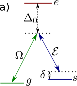
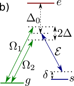
Figure 1: (Color online) Raman amplification schemes with a single probe field: Raman singlet (a) and Raman doublet (b)

First we consider the simplest Raman amplification scheme shown in Fig. 1a. Suppose there is an ensemble of atoms characterized by two hyperfine ground levels $g$ and $s$, and an electronic excited level $e$. The state of the atoms is described by atomic amplitudes $\Psi_{g}(\mathbf{r},t)$, $\Psi_{s}(\mathbf{r},t)$, $\Psi_{e}(\mathbf{r},t)$. The atoms interact with two light fields: a strong pump laser and a weaker probe field. Initially the atoms are in the ground level $g$ and we assume the Rabi frequency and duration of the probe pulse are small enough so that we can neglect the depletion of the ground level $g$. The propagation of the probe field inside of the atomic cloud we describe similarly as in Ref. Unanyan et al. (2010). We write the electric field of the probe beam in the form of a plane wave with modulated amplitude propagating along the $z$ axis:

$$\mathbf{E}(\mathbf{r},t)=\hat{\mathbf{e}}\sqrt{\frac{\hbar\omega}{2\varepsilon_{0}}}\mathcal{E}(\mathbf{r},t)e^{ikz-i\omega t}+\mathrm{H.c.}\,.$$ (4)

Here $\omega$ is the central frequency of the probe beam, $k=\omega/c$ is the corresponding wave vector, and $\hat{\mathbf{e}}\bot\hat{\mathbf{z}}$ is the unit polarization vector. The probe field $\mathbf{E}(\mathbf{r},t)$ obeys the following wave equation:

$$c^{2}\nabla^{2}\mathbf{E}-\frac{\partial^{2}}{\partial t^{2}}\mathbf{E}=\frac{1}{\varepsilon_{0}}\frac{\partial^{2}}{\partial t^{2}}\mathbf{P}\,,$$ (5)

where

$$\mathbf{P}=\hat{\mathbf{e}}\mu\Psi_{s}^{*}\Psi_{e}+\mathrm{H.c.}$$ (6)

is the polarization field of atoms, $\mu$ being the dipole moment for the atomic transition $s\rightarrow e$. The atomic amplitudes are normalized according to the equation $|\Psi_{g}|^{2}+|\Psi_{s}|^{2}+|\Psi_{e}|^{2}=n$, where $n$ is the atomic density. We introduce the slowly varying polarization $\mathcal{P}$ as:

$$\mathbf{P}=\hat{\mathbf{e}}\mathcal{P}e^{ikz-i\omega t}+\mathrm{H.c.}$$ (7)

Using Eq. (6) we get

$$\mathcal{P}=\mu\Psi_{s}^{*}\Psi_{e}e^{i\omega t-ikz}\,.$$ (8)

In case when the amplitude $\mathcal{E}$ varies slowly during the wavelength and optical cycle we can approximate Eq. (5) as Allen and Eberly (1975)

$$(\partial_{t}+c\partial_{z})\mathcal{E}=i\tilde{g}\mathcal{P}\,,$$ (9)

where

$$\tilde{g}=\sqrt{\frac{\omega}{2\varepsilon_{0}\hbar}}\,.$$ (10)

Let us introduce the slowly varying atomic amplitudes

$$\Phi_{g} = \Psi_{g}e^{i\omega_{g}t}\,,$$ (11)

$$\Phi_{s} = \Psi_{s}e^{i(\omega_{g}+\omega_{p}-\omega)t+ikz}\,,$$ (12)

$$\Phi_{e} = \Psi_{e}e^{i(\omega_{g}+\omega_{p})t}\,,$$ (13)

where $\hbar\omega_{g}$ is the energy of the atomic ground state $g$ and $\omega_{p}$ is the frequency of the pump field. Using the slowly varying atomic amplitudes and Eq. (8) the slowly varying polarization $\mathcal{P}$ can be written as

$$\mathcal{P}=\mu\Phi_{s}^{*}\Phi_{e}$$ (14)

The equations for the slowly varying atomic amplitudes are

$$i\partial_{t}\Phi_{e} = \Delta_{0}\Phi_{e}-g\mathcal{E}\Phi_{s}-\Omega\Phi_{g}\,,$$ (15)

$$i\partial_{t}\Phi_{s} = (\delta-i\gamma)\Phi_{s}-g\mathcal{E}^{*}\Phi_{e}\,,$$ (16)

where $\Omega$ is the Rabi frequency of the pump field,

$$\Delta_{0}=\omega_{e}-\omega_{g}-\omega_{p}$$ (17)

is one-photon detuning and

$$\delta=\omega-\omega_{p}+\omega_{s}-\omega_{g}$$ (18)

is two-photon detuning. Here $\hbar\omega_{e}$ and $\hbar\omega_{s}$ are energies of the atomic states $e$ and $s$. The parameter $\gamma$ characterizes the decay rate of the level $s$ and the parameter $g=\mu\tilde{g}$ characterizes the strength of coupling of the probe field with the atoms.

Let us consider monochromatic probe field for which the amplitude $\mathcal{E}$ is time-independent. We search for time-independent atomic amplitudes $\Phi_{g}$, $\Phi_{s}$ and $\Phi_{e}$, so that

$$c\partial_{z}\mathcal{E}-ig\Phi_{s}^{*}\Phi_{e} = 0$$ (19)

$$\Delta_{0}\Phi_{e}-g\mathcal{E}\Phi_{s}-\Omega\Phi_{g} = 0$$ (20)

$$(\delta-i\gamma)\Phi_{s}-g\mathcal{E}^{*}\Phi_{e} = 0$$ (21)

When one-photon detuning $\Delta_{0}$ is large, $\Delta_{0}|\delta-i\gamma|\gg g^{2}|\mathcal{E}|^{2}$ , Eq. (20) yields

$$\Phi_{e}=\frac{\Omega}{\Delta_{0}}\Phi_{g}\,.$$ (22)

Substituting Eq. (22) into Eq. (21) we get

$$\Phi_{s}=\frac{g\Phi_{g}\Omega}{\Delta_{0}(\delta-i\gamma)}\mathcal{E}^{*}\,.$$ (23)

Finally, using Eqs. (22), (23), and (19) we get the propagation equation for the electric field

$$c\partial_{z}\mathcal{E}-i\frac{g^{2}n|\Omega|^{2}}{\Delta_{0}^{2}(\delta+i\gamma)}\mathcal{E}=0\,.$$ (24)

Here we have taken into account that $|\Phi_{g}|^{2}=n$ in accordance with the adopted normalization. Plane waves

$$\mathcal{E}(z)=\mathcal{E}(0)e^{i\kappa z}$$ (25)

with

$$\kappa=\frac{g^{2}n|\Omega|^{2}}{c\Delta_{0}^{2}(\delta+i\gamma)}\,.$$ (26)

are the solutions of Eq. (24). Note, that $\kappa$ depends on the frequency $\omega$ of the probe field via the two-photon detuning $\delta$. The group velocity of the probe field in the medium can be determined from $\kappa(\omega)$. Since the fast-varying amplitude is proportional to $E(z,t)\sim\mathcal{E}(0)\exp\{i(\omega/c+\kappa(\omega))z-i\omega t\}$, the maximum of the wave packet made from such plane waves moves with the group velocity

$$v_{g}=c\left\{\frac{d(\omega+c\textrm{Re}\kappa(\omega))}{d\omega}\right\}^{-1}=\frac{c}{1+\frac{\partial}{\partial\omega}\textrm{Re}\left\{c\kappa(\omega)\right\}}\,.$$ (27)

Using Eq. (26) we get

$$v_{g}=\frac{c}{1+\frac{g^{2}n|\Omega|^{2}}{\Delta_{0}^{2}}\frac{\gamma^{2}-\delta^{2}}{(\delta^{2}+\gamma^{2})^{2}}}\,.$$ (28)

One can see that in the case $\gamma<\delta$ the group velocity exceeds $c$. This situation corresponds to the wings of the gain profile where the dispersion is anomalous. However, when two-photon detuning $\delta$ is close to zero, $v_{g}<c$. In order to improve this situation and have group velocity larger than $c$ in Ref. Steinberg and Chiao (1994) it was suggested to use two pump fields with different frequencies.

The amplitude of the probe field propagating through atomic cloud is changed. If the monochromatic probe field is incident on the atomic cloud, the amplitude of the transmitted field at the end of the atomic cloud becomes

$$\mathcal{E}(L)\sim\exp(i\kappa L)=\exp\left(i\frac{g^{2}n|\Omega|^{2}L}{c\Delta_{0}^{2}(\delta+i\gamma)}\right)\,.$$ (29)

By separating real and imaginary parts we obtain the transmission coefficient

$$R=\exp\left(\frac{|\Omega|^{2}}{\Delta_{0}^{2}}\frac{\gamma g^{2}nL}{c(\delta^{2}+\gamma^{2})}\right)=\exp\left(\frac{|\Omega|^{2}}{\Delta_{0}^{2}}\frac{L}{L_{\mathrm{dec}}}\frac{\gamma^{2}}{\delta^{2}+\gamma^{2}}\right)\,,$$ (30)

where

$$L_{\mathrm{dec}}=\frac{\gamma c}{g^{2}n}$$ (31)

is the characteristic length related to the decay of the level $s$. Since the expression in the exponent is positive, the transmission coefficient $R>1$, so there is an amplification of the probe beam.

II.1.2 Two pump fields (Raman doublet)

Now let us consider a situation where two strong pump beams (with frequencies $\omega_{p_{1}}$ and $\omega_{p_{2}}$ ) act on the atomic ensemble instead of one pump beam. This situation corresponds to a Raman gain doublet (Fig. 1b) and was investigated in Refs. Steinberg and Chiao (1994); Wang et al. (2000); Dogariu et al. (2001); Kuzmich et al. (2001). The consistent mathematical description of this case can be obtained using Floquet theory Chu and Telnov (2004). However, here we make use of a simpler approach. To describe the propagation of the probe beam in this scheme we separate the atomic amplitudes into two parts oscillating with different frequencies: $\Psi_{e}=\Psi_{e_{1}}+\Psi_{e_{2}}$, $\Psi_{s}=\Psi_{s_{1}}+\Psi_{s_{2}}$ with corresponding slowly changing amplitudes

$$\Phi_{e_{1}} = \Psi_{e_{1}}e^{i(\omega_{g}+\omega_{p_{1}})t}\,,\qquad\Phi_{e_{2}}=\Psi_{e_{2}}e^{i(\omega_{g}+\omega_{p_{2}})t}\,,$$

$$\Phi_{s_{1}} = \Psi_{s_{1}}e^{i(\omega_{g}+\omega_{p_{1}}-\omega)t+ikz}\,,\qquad\Phi_{s_{2}}=\Psi_{s_{2}}e^{i(\omega_{g}+\omega_{p_{2}}-\omega)t+ikz}\,.$$

After separating the atomic amplitudes into two parts, Eq. (8) yields the following relation for the slowly varying polarization:

$$\mathcal{P}=\mu(\Phi_{s_{1}}^{*}\Phi_{e_{1}}+\Phi_{s_{2}}^{*}\Phi_{e_{2}}+\Phi_{s_{1}}^{*}\Phi_{e_{2}}e^{-2i\Delta t}+\Phi_{s_{2}}^{*}\Phi_{e_{1}}e^{2i\Delta t})\,,$$ (32)

where

$$2\Delta=\omega_{p_{2}}-\omega_{p_{1}}\,.$$ (33)

Neglecting the terms oscillating with a large frequency $2\Delta$ which is still small compared to the one-photon detuning $\Delta_{0}$, one can write equations for the probe field and atomic amplitudes as

$$(\partial_{t}+c\partial_{z})\mathcal{E} = ig\Phi_{s_{1}}^{*}\Phi_{e_{1}}+ig\Phi_{s_{2}}^{*}\Phi_{e_{2}}\,,$$ (34)

$$i\partial_{t}\Phi_{e_{1}} = (\Delta_{0}-\Delta)\Phi_{e_{1}}-g\mathcal{E}\Phi_{s_{1}}-\Omega_{1}\Phi_{g}\,,$$ (35)

$$i\partial_{t}\Phi_{e_{2}} = (\Delta_{0}+\Delta)\Phi_{e_{2}}-g\mathcal{E}\Phi_{s_{2}}-\Omega_{2}\Phi_{g}\,,$$ (36)

$$i\partial_{t}\Phi_{s_{1}} = (\delta+\Delta-i\gamma)\Phi_{s_{1}}-g\mathcal{E}^{*}\Phi_{e_{1}}\,,$$ (37)

$$i\partial_{t}\Phi_{s_{2}} = (\delta-\Delta-i\gamma)\Phi_{s_{2}}-g\mathcal{E}^{*}\Phi_{e_{2}}\,.$$ (38)

Here

$$\Delta_{0}=\omega_{e}-\omega_{g}-\frac{1}{2}(\omega_{p_{1}}+\omega_{p_{2}})$$ (39)

is an average one-photon detuning and

$$\delta=\omega-\frac{1}{2}(\omega_{p_{1}}+\omega_{p_{2}})+\omega_{s}-\omega_{g}$$ (40)

is an average two-photon detuning. Proceeding similarly as in the case of one pump field we obtain the following set of equations for the time-independent complex amplitudes in the case of large $\Delta_{0}$:

$$c\partial_{z}\mathcal{E} = ig\Phi_{s_{1}}^{*}\frac{\Omega_{1}}{\Delta_{0}}\Phi_{g}+ig\Phi_{s_{2}}^{*}\frac{\Omega_{1}}{\Delta_{0}}\Phi_{g}\,,$$ (41)

$$\Phi_{s_{1}} = \frac{g\Omega_{1}}{\Delta_{0}(\delta+\Delta-i\gamma)}\Phi_{g}\mathcal{E}^{*}\,,$$ (42)

$$\Phi_{s_{2}} = \frac{g\Omega_{2}}{\Delta_{0}(\delta-\Delta-i\gamma)}\Phi_{g}\mathcal{E}^{*}\,.$$ (43)

From Eqs. (41)–(43) follows the equation for the probe field

$$c\partial_{z}\mathcal{E}-i\frac{g^{2}n}{\Delta_{0}^{2}}\left[\frac{|\Omega_{1}|^{2}}{\delta+\Delta+i\gamma}+\frac{|\Omega_{2}|^{2}}{\delta-\Delta+i\gamma}\right]\mathcal{E}=0\,.$$ (44)

Searching for the plane wave solution we find

$$\kappa=\frac{g^{2}n}{c\Delta_{0}^{2}}\left[\frac{|\Omega_{1}|^{2}}{\delta+\Delta+i\gamma}+\frac{|\Omega_{2}|^{2}}{\delta-\Delta+i\gamma}\right]\,.$$ (45)

In a particular case where $|\Omega_{1}|=|\Omega_{2}|$ and $\delta=0$ one finds

$$\frac{\partial}{\partial\omega}\textrm{Re}\left\{c\kappa(\omega)\right\}=-2g^{2}n\frac{|\Omega_{1}|^{2}}{\Delta_{0}^{2}}\frac{\Delta^{2}-\gamma^{2}}{(\Delta^{2}+\gamma^{2})^{2}}\,.$$ (46)

Thus for $\Delta>\gamma$ the group velocity is larger than $c$. We see that, in contrast to the scheme with a single pump field, we have superluminal propagation even for zero two-photon detuning $\delta$.

II.2 Two probe fields

II.2.1 Two pump fields

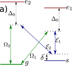
Figure 2: (Color online) Raman amplification schemes with two probe fields: double Raman singlet (a) and double Raman doublet (b)

Now we shall turn to the main goal of this article by studying the propagation of two probe fields in Raman gain situation. Thus we consider an ensemble of atoms characterized by two hyperfine ground levels $g$, $s$ and two electronic excited levels $e_{1}$ and $e_{2}$. The state of the atoms is described by the atomic amplitudes $\Psi_{g}(\mathbf{r},t)$, $\Psi_{s}(\mathbf{r},t)$, $\Psi_{e_{1}}(\mathbf{r},t)$, $\Psi_{e_{2}}(\mathbf{r},t)$. Similarly to the single probe field we first investigate a simpler scheme where the atoms interact with four light fields: two strong pump lasers and two weaker probe fields (Fig. 2a). We assume the four photon resonance condition

$$\omega_{1}-\omega_{p_{1}}=\omega_{2}-\omega_{p_{2}}\,,$$ (47)

where $\omega_{1}$ and $\omega_{2}$ are frequencies of the probe beams, $\omega_{p_{1}}$ and $\omega_{p_{2}}$ are frequencies of the pump beams.

For each probe beam we introduce slowly varying amplitudes $\mathcal{E}_{1}$ and $\mathcal{E}_{2}$ of the electric field according to Eq. (4). Wave vectors of the probe fields are $k_{1}=\omega_{1}/c$ and $k_{2}=\omega_{2}/c$ . The wave equations and the corresponding polarization fields are written separately for each of the probe field similarly to Eqs. (5) and (6). In the following, the strength of coupling of probe fields with the atoms is assumed to be the same for both probe fields: $g=\mu_{1}\sqrt{\omega_{1}/2\varepsilon_{0}\hbar}=\mu_{2}\sqrt{\omega_{2}/2\varepsilon_{0}\hbar}\,,$where $\mu_{1}$ and $\mu_{2}$ denote the dipole momenta for the atomic transitions $s\rightarrow e_{1}$ and $s\rightarrow e_{2}$, respectively. After introducing the slowly varying atomic amplitudes we obtain the following equations for slowly varying probe field amplitudes $\mathcal{E}_{1}$ and $\mathcal{E}_{2}$ :

$$(\partial_{t}+c\partial_{z})\mathcal{E}_{1} = ig\Phi_{s}^{*}\Phi_{e_{1}}\,,$$ (48)

$$(\partial_{t}+c\partial_{z})\mathcal{E}_{2} = ig\Phi_{s}^{*}\Phi_{e_{2}}\,.$$ (49)

On the other hand, the equations for the atomic amplitudes are

$$i\partial_{t}\Phi_{e_{1}} = \Delta_{0}\Phi_{e_{1}}-g\mathcal{E}_{1}\Phi_{s}-\Omega_{1}\Phi_{g}\,,$$ (50)

$$i\partial_{t}\Phi_{e_{2}} = \Delta_{0}\Phi_{e_{2}}-g\mathcal{E}_{2}\Phi_{s}-\Omega_{2}\Phi_{g}\,,$$ (51)

$$i\partial_{t}\Phi_{s} = (\delta-i\gamma)\Phi_{s}-g\mathcal{E}_{1}^{*}\Phi_{e_{1}}-g\mathcal{E}_{2}^{*}\Phi_{e_{2}}\,,$$ (52)

where

$$\Delta_{0}=\omega_{e_{1}}-\omega_{g}-\omega_{p_{1}}=\omega_{e_{2}}-\omega_{g}-\omega_{p_{2}}$$ (53)

is one-photon detuning and

$$\delta=\omega_{1}-\omega_{p_{1}}+\omega_{s}-\omega_{g}=\omega_{2}-\omega_{p_{2}}+\omega_{s}-\omega_{g}$$ (54)

is two-photon detuning. Here $\hbar\omega_{e_{1}}$, $\hbar\omega_{e_{2}}$ and $\hbar\omega_{s}$ are energies of the atomic states $e_{1}$, $e_{2}$ and $s$, respectively.

As before, we consider the case of monochromatic probe beams with time independent amplitudes $\mathcal{E}_{1}$, $\mathcal{E}_{2}$ and the constant atomic amplitudes $\Phi_{g}$, $\Phi_{s}$, $\Phi_{e_{1}}$ and $\Phi_{e_{2}}$. Assuming a large detuning, $\Delta_{0}|\delta-i\gamma|\gg g^{2}|\mathcal{E}|^{2}$, the corresponding equations for the atomic amplitudes reduce to

$$\Phi_{e_{1}} = \frac{\Omega_{1}}{\Delta_{0}}\Phi_{g}\,,$$ (55)

$$\Phi_{e_{2}} = \frac{\Omega_{2}}{\Delta_{0}}\Phi_{g}\,.$$ (56)

and

$$\Phi_{s}=\frac{g\Phi_{g}}{\Delta_{0}(\delta-i\gamma)}(\Omega_{1}\mathcal{E}_{1}^{*}+\Omega_{2}\mathcal{E}_{2}^{*})\,.$$ (57)

Substituting these relations into the equations for the fields $\mathcal{E}_{1}$ and $\mathcal{E}_{2}$, we get

$$c\partial_{z}\mathcal{E}_{1}-i\frac{g^{2}n\Omega_{1}}{\Delta_{0}^{2}(\delta+i\gamma)}(\Omega_{1}^{*}\mathcal{E}_{1}+\Omega_{2}^{*}\mathcal{E}_{2}) = 0\,,$$ (58)

$$c\partial_{z}\mathcal{E}_{2}-i\frac{g^{2}n\Omega_{2}}{\Delta_{0}^{2}(\delta+i\gamma)}(\Omega_{1}^{*}\mathcal{E}_{1}+\Omega_{2}^{*}\mathcal{E}_{2}) = 0\,.$$ (59)

Introducing new fields representing superpositions of the original probe fields

$$\psi = \frac{1}{\Omega}(\Omega_{1}^{*}\mathcal{E}_{1}+\Omega_{2}^{*}\mathcal{E}_{2})\,,$$ (60)

$$\phi = \frac{1}{\Omega}(\Omega_{2}\mathcal{E}_{1}-\Omega_{1}\mathcal{E}_{2})\,,$$ (61)

Eqs. (58) and (59) take the form

$$c\partial_{z}\psi-i\frac{g^{2}n\Omega^{2}}{\Delta_{0}^{2}(\delta+i\gamma)}\psi = 0\,,$$ (62)

$$c\partial_{z}\phi = 0\,,$$ (63)

where

$$\Omega=\sqrt{|\Omega_{1}|^{2}+|\Omega_{2}|^{2}}$$ (64)

is the total Rabi frequency. One can see that the field $\phi$ propagates like in free space without interacting with the atoms. The other field $\psi$ does interact with the atoms. The solutions of Eq. (62) are plane waves:

$$\psi(z)=\psi(0)e^{i\kappa z}\,,$$ (65)

with

$$\kappa=\frac{g^{2}n\Omega^{2}}{c\Delta_{0}^{2}(\delta+i\gamma)}\,.$$ (66)

This result coincides with the Eq. (26), implying that the group velocity has the form of Eq. (28). For $\gamma<\delta$ the group velocity exceeds the vacuum speed of light.

II.2.2 Four pump fields (double Raman doublet)

Let us now consider a situation where four strong pump beams act on the atomic ensemble. This situation corresponds to a Raman gain doublet for each of the probe beams (Fig. 2b). We assume four-photon resonances

$$\omega_{p_{1,1}}-\omega_{1} = \omega_{p_{2,1}}-\omega_{2}\,,$$ (67)

$$\omega_{p_{1,2}}-\omega_{1} = \omega_{p_{2,2}}-\omega_{2}\,,$$ (68)

where $\omega_{p_{1,1}}$, $\omega_{p_{1,2}}$, $\omega_{p_{2,1}}$ and $\omega_{p_{2,2}}$ are the frequencies of the pump beams. Similarly as in the scheme with the single probe beam we write the atomic amplitudes as a sum of two parts: $\Psi_{e_{1}}=\Psi_{e_{1,1}}+\Psi_{e_{1,2}}$, $\Psi_{e_{2}}=\Psi_{e_{2,1}}+\Psi_{e_{2,2}}$, $\Psi_{s}=\Psi_{s_{1}}+\Psi_{s_{2}}$. Introducing the slowly changing amplitudes and neglecting the terms oscillating with the frequency

$$2\Delta=\omega_{p_{1,2}}-\omega_{p_{1,1}}=\omega_{p_{2,2}}-\omega_{p_{2,1}}$$ (69)

we find the following set of equations

$$c\partial_{z}\mathcal{E}_{1} = ig\Phi_{s_{1}}^{*}\frac{\Omega_{1,1}}{\Delta_{0}}\Phi_{g}+ig\Phi_{s_{2}}^{*}\frac{\Omega_{1,2}}{\Delta_{0}}\Phi_{g}$$ (70)

$$c\partial_{z}\mathcal{E}_{2} = ig\Phi_{s_{1}}^{*}\frac{\Omega_{2,1}}{\Delta_{0}}\Phi_{g}+ig\Phi_{s_{2}}^{*}\frac{\Omega_{2,2}}{\Delta_{0}}\Phi_{g}$$ (71)

$$\Phi_{s_{1}} = \frac{g\Phi_{g}}{(\delta+\Delta-i\gamma)\Delta_{0}}(\Omega_{1,1}\mathcal{E}_{1}^{*}+\Omega_{2,1}\mathcal{E}_{2}^{*})$$ (72)

$$\Phi_{s_{2}} = \frac{g\Phi_{g}}{(\delta-\Delta-i\gamma)\Delta_{0}}(\Omega_{1,2}\mathcal{E}_{1}^{*}+\Omega_{2,2}\mathcal{E}_{2}^{*})$$ (73)

for the amplitudes of the monochromatic probe fields and the time independent atomic amplitudes. Here

$$\Delta_{0}=\omega_{e_{1}}-\omega_{g}-\frac{1}{2}(\omega_{p_{1,1}}+\omega_{p_{1,2}})=\omega_{e_{2}}-\omega_{g}-\frac{1}{2}(\omega_{p_{2,1}}+\omega_{p_{2,2}})$$ (74)

is an average two-photon detuning and

$$\delta=\omega_{1}-\frac{1}{2}(\omega_{p_{1,1}}+\omega_{p_{1,2}})+\omega_{s}-\omega_{g}=\omega_{2}-\frac{1}{2}(\omega_{p_{2,1}}+\omega_{p_{2,2}})+\omega_{s}-\omega_{g}$$ (75)

is an average two-photon detuning. From Eqs. (70)–(73) we obtain the equations of propagation of the probe fields

$$c\partial_{z}\mathcal{E}_{1} = i\frac{g^{2}n}{\Delta_{0}^{2}}\left[\frac{\Omega_{1,1}(\Omega_{1,1}^{*}\mathcal{E}_{1}+\Omega_{2,1}^{*}\mathcal{E}_{2})}{(\delta+\Delta+i\gamma)}+\frac{\Omega_{1,2}(\Omega_{1,2}^{*}\mathcal{E}_{1}+\Omega_{2,2}^{*}\mathcal{E}_{2})}{(\delta-\Delta+i\gamma)}\right]\,,$$ (76)

$$c\partial_{z}\mathcal{E}_{2} = i\frac{g^{2}n}{\Delta_{0}^{2}}\left[\frac{\Omega_{2,1}(\Omega_{1,1}^{*}\mathcal{E}_{1}+\Omega_{2,1}^{*}\mathcal{E}_{2})}{(\delta+\Delta+i\gamma)}+\frac{\Omega_{2,2}(\Omega_{1,2}^{*}\mathcal{E}_{1}+\Omega_{2,2}^{*}\mathcal{E}_{2})}{(\delta-\Delta+i\gamma)}\right]\,.$$ (77)

Let us consider a particular situation in which

$$\frac{\Omega_{1,2}}{\Omega_{1,1}}=\frac{\Omega_{2,2}}{\Omega_{2,1}}\,.$$ (78)

Introducing new fields

$$\psi = \frac{1}{\Omega_{1}}(\Omega_{1,1}^{*}\mathcal{E}_{1}+\Omega_{2,1}^{*}\mathcal{E}_{2})$$ (79)

$$\phi = \frac{1}{\Omega_{1}}(\Omega_{2,1}\mathcal{E}_{1}-\Omega_{1,1}\mathcal{E}_{2})$$ (80)

we get the equations for the fields $\psi$ and $\phi$:

$$c\partial_{z}\psi-i\frac{g^{2}n}{\Delta_{0}^{2}}\left[\frac{\Omega_{1}^{2}}{\delta+\Delta+i\gamma}+\frac{\Omega_{2}^{2}}{\delta-\Delta+i\gamma}\right]\psi = 0\,,$$ (81)

$$c\partial_{z}\phi = 0\,,$$ (82)

where

$$\Omega_{1} = \sqrt{|\Omega_{1,1}|^{2}+|\Omega_{2,1}|^{2}}$$ (83)

$$\Omega_{2} = \sqrt{|\Omega_{1,2}|^{2}+|\Omega_{2,2}|^{2}}$$ (84)

The field $\phi$ propagates without interaction with atoms. The plane wave solution of Eq. (81) gives

$$\kappa=\frac{g^{2}n}{c\Delta_{0}^{2}}\left[\frac{|\Omega_{1}|^{2}}{\delta+\Delta+i\gamma}+\frac{|\Omega_{2}|^{2}}{\delta-\Delta+i\gamma}\right]\,.$$ (85)

This quantity corresponds to Eq. (45) providing a superluminal propagation.

III Propagation of probe beam wave packets

To illustrate the superluminal behavior of the probe pulses, in this Section we will consider the propagation of a Gaussian wave packet through the atomic cloud. The wave packet is formed by taking a superposition of monochromatic solutions of the propagation equations. The length of the atomic cloud is $L$. For simplicity we will measure all frequencies in units of $\gamma$ and time in units of $\gamma^{-1}$ and set $\gamma=1$. Furthermore, by measuring the length in the units of $c/\gamma$, we set $c=1$.

III.1 Single probe field

At first we will consider the propagation of the incident Gaussian wave packet for a scheme with a single probe beam and a Raman gain doublet, as shown in Fig. 1b. The fast-varying amplitude of the monochromatic probe field is

$$E_{\delta}(z,t)=\begin{cases}\mathcal{E}_{\delta}e^{i\delta z-i\delta t}\,,&z\leqslant 0\\ \mathcal{E}_{\delta}e^{i(\delta+\kappa(\delta))z-i\delta t}\,,&0<z<L\\ \mathcal{E}_{\delta}e^{i\kappa(\delta)L+i\delta z-i\delta t}\,,&L\leqslant z\,.\end{cases}$$ (86)

Here we have used the two-photon detuning $\delta$ (40) instead of the frequency $\omega$ . The change of the wave number $\kappa(\delta)$ is given by Eq. (45). When $\Omega_{1}=\Omega_{2}$ we can write

$$\kappa=M\left[\frac{1}{\delta+\Delta+i}+\frac{1}{\delta-\Delta+i}\right]\,,$$ (87)

with

$$M=\frac{1}{L_{\mathrm{dec}}}\frac{|\Omega_{1}|^{2}}{\Delta_{0}^{2}}\,.$$ (88)

Here $L_{\mathrm{dec}}$ is the length defined by Eq. (31). At the central frequency $\delta=0$ the group velocity is

$$v_{g}=\frac{1}{1+\kappa^{\prime}(0)}=\frac{1}{1-2M\frac{\Delta^{2}-1}{(\Delta^{2}+1)^{2}}}\,.$$ (89)

In order to get the group velocity larger than $1$ (i.e. larger than $c=1$), the dimensionless one-photon detuning should be $\Delta>1$. The group velocity is maximum when $\Delta=\sqrt{3}$. For this value of $\Delta$ it is $v_{g}=(1-M/4)^{-1}$. If $M>4$, we have a negative group velocity. For $\delta=0$ the transmission coefficient is

$$R=\exp(i\kappa(0)L)=\exp\left(ML\frac{2}{\Delta^{2}+1}\right)\,.$$ (90)

In particular, for $\Delta=\sqrt{3}$ , the transmission coefficient is $R=\exp(ML/2)$.

The Gaussian wave packet can be formed by taking a superposition of monochromatic waves (86)

$$E(z,t)=\int_{-\infty}^{+\infty}E_{\delta}(z,t)\,d\delta\,,$$ (91)

with

$$\mathcal{E}_{\delta}=\frac{1}{\sqrt{\pi}\sigma}\exp\left(-\frac{\delta^{2}}{\sigma^{2}}-i\delta z_{0}\right)\,,$$ (92)

where $z_{0}$ is a location of the initial wavepacket peak, and $\sigma$ is the width of the packet in the frequency domain. To be in the dispersion region with a negative slope, the width $\sigma$ should be smaller than approximately $0.8$. Using Eq. (92) the incident probe field reads

$$E(z,t)=\exp\left[-\frac{\sigma^{2}}{4}(z-z_{0}-t)^{2}\right]\,.$$ (93)

From this equation we see that the width of the wave packet in the coordinate space is

$$\sigma_{z}=\frac{2}{\sigma}\,.$$ (94)

To avoid tails of the initial wave packet in the atomic cloud, we need to have $|z_{0}|\gg\sigma_{z}$.

For a Gaussian packet narrow in the frequency space, we can obtain approximate expressions for the electric field by expanding $\kappa(\delta)$ in power series and taking the first three terms:

$$\kappa(\delta)\approx\kappa(0)+\kappa^{\prime}(0)\delta+\kappa^{\prime\prime}\delta^{2}/2\,,$$ (95)

with

$$\kappa(0) = -2i\frac{M}{\Delta^{2}+1}$$ (96)

$$\kappa^{\prime}(0) = -2M\frac{\Delta^{2}-1}{(\Delta^{2}+1)^{2}}$$ (97)

$$\kappa^{\prime\prime}(0) = -4iM\frac{3\Delta^{2}-1}{(\Delta^{2}+1)^{3}}$$ (98)

Nonlinear terms in the expansion are associated with group velocity dispersion and cause pulse distortion. After performing the integration we get approximate expressions for the probe field. The probe field is

$$E_{\mathrm{inside}}(z,t)\approx\frac{1}{\sqrt{1-i\frac{1}{2}\kappa^{\prime\prime}(0)\sigma^{2}z}}\exp\left(-\frac{\sigma^{2}[(1+\kappa^{\prime}(0))z-z_{0}-t]^{2}}{4\left(1-i\frac{1}{2}\kappa^{\prime\prime}(0)\sigma^{2}z\right)}+i\kappa(0)z\right)$$ (99)

inside the atomic medium and

$$E_{\mathrm{outside}}(z,t)\approx\frac{1}{\sqrt{1-i\frac{1}{2}\kappa^{\prime\prime}(0)\sigma^{2}L}}\exp\left(-\frac{\sigma^{2}[z+\kappa^{\prime}(0)L-z_{0}-t]^{2}}{4\left(1-i\frac{1}{2}\kappa^{\prime\prime}(0)\sigma^{2}L\right)}+i\kappa(0)L\right)$$ (100)

outside the atomic cloud. From Eq. (100) it follows that the distortion of the pulse is determined by the parameter $[1-i\kappa^{\prime\prime}(0)\sigma^{2}L/2]^{-1/2}$ Dogariu et al. (2001).

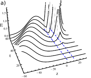
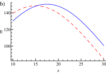
Figure 3: (Color online) Propagation of the incoming Gaussian wave packet, described by Eq. (93) through atomic cloud, calculated using Eqs. (86), (91), (92). All the quantities shown are dimensionless. (a) Time evolution of the probe field. Dashed blue lines show the location of the atomic cloud. (b) Comparison of the transmitted wave packet (solid blue line) with the wave packet propagating in the vacuum (dashed red line) at the same time moment $t=90$. In order to make the amplitudes of the wave packets similar, the amplitude of the Gaussian packet propagating in the vacuum is increased by the factor $R$ given by Eq. (90). The parameters used in calculation are $\sigma=0.1$, $z_{0}=-75$, $\Delta=\sqrt{3}$, $M=1$; the length of the atomic cloud is $L=10$. At these parameters the group velocity is $v_{g}=1.33$ and transmission coefficient $R=148.4$.

Propagation of the Gaussian wave packet, described by Eq. (93), through atomic cloud is shown in Fig. 3. As one can see in Fig. 3a, the front tail of the wave packet, entering the atomic cloud gets amplified and develops a maximum at the other end of the atomic cloud. Comparison of the transmitted wave packet with the wave packet propagating in the vacuum at the same time moment is shown in Fig. 3b. In order to make the amplitudes of the wave packets similar, the amplitude of the wave packet propagating in the vacuum is increased by the factor $R$ given by Eq. (90). One can see that the maximum of the wave packet after the atomic cloud is located at larger value of the coordinate $z$ than the maximum of the wave packet propagating in the vacuum. This is a signature of the superluminal group velocity, $v_{g}>1$.

III.2 Two probe fields

Next let us consider the propagation of the incident Gaussian wave packet for the scheme with four pump beams (two Raman gain doublets), shown in Fig. 2b. At first we will consider propagation of monochromatic probe fields. Let us assume that only one probe field $\mathcal{E}_{1}$ is incident on the atomic cloud. The amplitude of this probe field at the beginning of the atomic cloud is $\mathcal{E}_{1}(z=0)\equiv\mathcal{E}_{\delta}$. Here we use the two-photon detuning

$$\delta=\omega_{1}-\frac{1}{2}(\omega_{p_{1,1}}+\omega_{p_{1,2}})+\omega_{s}-\omega_{g}=\omega_{2}-\frac{1}{2}(\omega_{p_{2,1}}+\omega_{p_{2,2}})+\omega_{s}-\omega_{g}\,.$$ (101)

instead of the frequencies $\omega_{1}$ and $\omega_{2}$. The fields $\psi$ and $\phi$, introduced by Eqs. (79), (80), at the beginning of the atomic cloud are

$$\psi(z=0) = \frac{\Omega_{1,1}^{*}}{\Omega}\mathcal{E}_{\delta}\,,$$ (102)

$$\phi(z=0) = \frac{\Omega_{2,1}}{\Omega}\mathcal{E}_{\delta}\,.$$ (103)

Inside the atomic cloud the fields $\psi$ and $\phi$ depend on the coordinate $z$ according to $\phi(z)=\phi(0)$ and $\psi(z)=\psi(0)e^{i\kappa z}$, with $\kappa$ given by Eq. (85). Thus, at the end of the cloud the fields $\psi$ and $\phi$ are $\phi(L)=\phi(0)$ and $\psi(L)=e^{i\kappa L}\psi(0)$ . We will consider only the case when $\Omega_{1}=\Omega_{2}$. Then the expression for the wave number $\kappa(\delta)$ is the same as in the scheme with the single probe beam and is given by Eq. (87). The electric fields of the probe beams inside the atomic cloud can be obtained from the fields $\psi$ and $\phi$:

$$\mathcal{E}_{1}(z) = \frac{1}{\Omega_{1}}(\Omega_{1,1}\psi(z)+\Omega_{2,1}^{*}\phi(z))=\left(1+\frac{|\Omega_{1,1}|^{2}}{\Omega_{1}^{2}}(e^{i\kappa z}-1)\right)\mathcal{E}_{\delta}\,,$$ (104)

$$\mathcal{E}_{2}(z) = \frac{1}{\Omega_{1}}(\Omega_{2,1}\psi(z)-\Omega_{1,1}^{*}\phi(z))=\frac{\Omega_{2,1}\Omega_{1,1}^{*}}{\Omega_{1}^{2}}(e^{i\kappa z}-1)\mathcal{E}_{\delta}\,.$$ (105)

Using Eqs. (104), (105), the fast-varying amplitude of the monochromatic probe fields are

$$E_{1,\delta}(z,t) = \begin{cases}\mathcal{E}_{\delta}e^{i\delta z-i\delta t}\,,&z\leqslant 0\,,\\ \left(1+\frac{|\Omega_{1,1}|^{2}}{\Omega_{1}^{2}}(e^{i\kappa(\delta)z}-1)\right)\mathcal{E}_{\delta}e^{i\delta z-i\delta t}\,,&0<z<L\,,\\ \left(1+\frac{|\Omega_{1,1}|^{2}}{\Omega_{1}^{2}}(e^{i\kappa(\delta)L}-1)\right)\mathcal{E}_{\delta}e^{i\delta z-i\delta t}\,,&L\leqslant z\,,\end{cases}$$ (106)

$$E_{2,\delta}(z,t) = \begin{cases}0\,,&z\leqslant 0\,,\\ \frac{\Omega_{2,1}\Omega_{1,1}^{*}}{\Omega_{1}^{2}}(e^{i\kappa(\delta)z}-1)\mathcal{E}_{\delta}e^{i\delta z-i\delta t}\,,&0<z<L\,,\\ \frac{\Omega_{2,1}\Omega_{1,1}^{*}}{\Omega_{1}^{2}}(e^{i\kappa(\delta)L}-1)\mathcal{E}_{\delta}e^{i\delta z-i\delta t}\,,&L\leqslant z\,.\end{cases}$$ (107)

The amplitude of the second probe field $\mathcal{E}_{2}$ at the other side of the atomic cloud is maximal when $|\Omega_{1,1}|/\Omega_{1}=|\Omega_{2,1}|/\Omega_{1}=1/\sqrt{2}$.

The Gaussian wave packet can be formed by taking superpositions of monochromatic waves (106), (107)

$$E_{1}(z,t) = \int_{-\infty}^{+\infty}E_{1,\delta}(z,t)\,d\delta$$ (108)

$$E_{2}(z,t) = \int_{-\infty}^{+\infty}E_{2,\delta}(z,t)\,d\delta$$ (109)

with $\mathcal{E}_{\delta}$ given by Eq. (92). In this case the electric field of the first probe beam in the free space before the atomic cloud is given by Eq. (93). After performing the integration we obtain

$$E_{1}(z,t) = \frac{|\Omega_{2,1}|^{2}}{\Omega_{1}^{2}}\exp\left(-\frac{\sigma^{2}}{4}(z-z_{0}-t)^{2}\right)+\frac{|\Omega_{1,1}|^{2}}{\Omega_{1}^{2}}E_{\mathrm{inside}}(z,t)$$ (110)

$$E_{2}(z,t) = \frac{\Omega_{2,1}\Omega_{1,1}^{*}}{\Omega_{1}^{2}}\left[E_{\mathrm{inside}}(z,t)-\exp\left(-\frac{\sigma^{2}}{4}(z-z_{0}-t)^{2}\right)\right]$$ (111)

for the probe fields inside of the atomic cloud and

$$E_{1}(z,t) = \frac{|\Omega_{2,1}|^{2}}{\Omega_{1}^{2}}\exp\left(-\frac{\sigma^{2}}{4}(z-z_{0}-t)^{2}\right)+\frac{|\Omega_{1,1}|^{2}}{\Omega_{1}^{2}}E_{\mathrm{outside}}(z,t)$$ (112)

$$E_{2}(z,t) = \frac{\Omega_{2,1}\Omega_{1,1}^{*}}{\Omega_{1}^{2}}\left[E_{\mathrm{outside}}(z,t)-\exp\left(-\frac{\sigma^{2}}{4}(z-z_{0}-t)^{2}\right)\right]$$ (113)

for the probe fields at the other side of the atomic cloud. Here $E_{\mathrm{inside}}(z,t)$ and $E_{\mathrm{outside}}(z,t)$ are, respectively, the probe field inside of the atomic cloud and after passing the atomic cloud in the scheme with the single Raman gain doublet. For the incident Gaussian packet narrow in the frequency space we can obtain approximate expressions for the electric fields by expanding $\kappa(\delta)$ in power series. Then $E_{\mathrm{inside}}(z,t)$ and $E_{\mathrm{outside}}(z,t)$ are given by Eqs. (99) and (100).

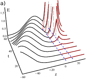
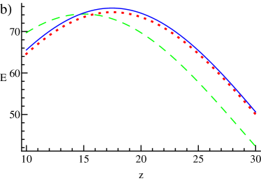
Figure 4: (Color online) Propagation through the atomic cloud of the incoming Gaussian wave packet (93) in the first probe field $\mathcal{E}_{1}$ and the creation of the second probe field $\mathcal{E}_{2}$ for the scheme with two Raman gain doublets, calculated using Eqs. (106), (107), (108), (109), (92). All the quantities shown are dimensionless. (a) Evolution of the probe fields with time. Solid black line shows the first probe field, dotted red line shows the second probe field. Dashed blue lines indicate the location of the atomic cloud. (b) Comparison of the wave packet of the first probe beam (solid blue line) and the second probe beam (dotted red line) with the incident wave packet of the first beam propagating in the vacuum (dashed green line) at the same time moment $t=90$. In order to make the amplitudes of the wave packets similar, the amplitude of the Gaussian packet propagating in the vacuum is increased by the factor $0.5R$, with $R$ given by Eq. (90). The parameters used in calculation are $\Omega_{1,1}/\Omega_{1}=\Omega_{2,1}/\Omega_{1}=1/\sqrt{2}$, all other prameters are the same as in Fig. 3.

The Fig. 4 illustrates the evolution of the probe fields in the scheme with two Raman gain doublets when the first probe field representing the Gaussian wave packet (93) is incident on the atomic cloud. As one can see in Fig. 4a, the front tail of the wave packet, entering the atomic cloud gets amplified and develops a maximum at the other end of the atomic cloud. In addition, the second probe field is created and also gets amplified, reaching the maximum at the other end of the atomic cloud. The Fig. 4b compares the wave packets of the probe beams after exiting the atomic cloud with the incoming wave packet of the first probe beam propagating in the vacuum. In order to make the amplitudes of the wave packets similar, the amplitude of the wave packet propagating in the vacuum is increased by the factor $0.5R$ given by Eq. (90). The factor $0.5$ is needed because the energy in the scheme with two Raman gain doublets is transferred to two probe beams, instead of one beam in the scheme with single Raman gain doublet. After exiting the atomic cloud, the maximum of the wave packet of the first probe beam is seen to be located at larger value of the coordinate $z$ than the maximum of the wave packet propagating in the vacuum, indicating the superluminal group velocity $v_{g}>1$. The maximum of the second probe beam after the atomic cloud is almost at the same location as the maximum of the first probe beam.

IV Concluding remarks

We have demonstrated a possibility of producing superluminal light composed of two probe waves characterized by different frequencies and propagating in a medium with two Raman gain doublets. Although individual probe fields exhibit Raman gain, a strong connection is established between two probe fields due to the resonance between real and virtual states in the coupling scheme. This leads to the formation of a specific combination (superposition) of the probe field envelopes propagating with a definite group velocity determined by the pump power and the detunings. Such a regime corresponds to the pulse propagation with a superluminal velocity and mathematically is described by a particular solution of the wave equation. It is shown that a peak of the superluminal wavepacket is advanced with respect to the corresponding pulse propagating in the vacuum. Additionally, it is demonstrated that if only one probe field is incident on the medium, both frequencies are produced at the end of the medium as a result of the coupling between the individual probe fields. Two-frequency superluminal light extends possibilities to control light pulses and their interactions in optical media.

The scheme for creating a two-component superluminal light, shown in Fig. 2b, can be experimentally implemented using an atomic cesium (Cs) vapor cell at the room temperature, as in the experiment by Wang et all. Wang et al. (2000) on the single-component superluminal light. All cesium atoms are to be prepared in the ground-state hyper-fine magnetic sublevel $6\mathrm{S}_{1/2}$, $|F=4,m=-4\rangle$ serving as the level $g$ in our scheme. The magnetic sublevel $6\mathrm{S}_{1/2}$, $|F=4,m=-2\rangle$ corresponds to the level $s$. On the other hand, the states $6\mathrm{P}_{3/2}$, $|F=4,m=-3\rangle$ and $6\mathrm{P}_{1/2}$, $|F=4,m=-3\rangle$ can be chosen to be the excited levels $e_{1}$ and $e_{2}$, respectively. The strong Raman pump beams should be right-hand polarized ($\sigma^{+}$) and two weak Raman probe beams should be left-hand polarized ($\sigma^{-}$) to couple properly the atomic levels. To create the two-component supeluminal light, one can also make use of other atoms, such as the rubidium ${}^{87}\mathrm{Rb}$ with the following hyper-fine magnetic sublevels involved: $5\mathrm{S}_{1/2}$, $|F=2,m=-2\rangle$ as the ground level $g$, $5\mathrm{S}_{1/2}$, $|F=2,m=0\rangle$ as the level $s$, $5\mathrm{P}_{1/2}$, $|F=2,m=-1\rangle$ and $5\mathrm{P}_{3/2}$, $|F=2,m=-1\rangle$ as the excited levels $e_{1}$ and $e_{2}$.

References

• Rayleigh (1899) L. Rayleigh, Philos. Mag. XLVIII, 151 (1899).
• Brillouin (1960) L. Brillouin, Wave Propagation and Group Velocity (Academic Press, New York, 1960).
• Born and Wolf (1997) M. Born and E. Wolf, Principles of Optics, 7th ed. (Cambridge University Press, Cambridge, 1997).
• Ware et al. (2001) M. Ware, S. Glasgow,  and J. Peatross, Opt. Expr. 9, 519 (2001).
• Stenner et al. (2003) M. D. Stenner, D. J. Gauthier,  and M. A. Neifeld, Nature 425, 695 (2003).
• Milonni (2005) P. W. Milonni, Fast Light, Slow Light, Left-Handed Light (Institute of Physics, Bristol, UK, 2005).
• Arimondo (1996) E. Arimondo, “Progress in optics,”  (Elsevier, Amsterdam, 1996) p. 257.
• Harris (1997) S. E. Harris, Phys. Today 50, 36 (1997).
• Scully and Zubairy (1997) M. O. Scully and M. S. Zubairy, Quantum Optics (Cambridge University Press, Cambridge, 1997).
• Lukin (2003) M. D. Lukin, Rev. Mod. Phys. 75, 457 (2003).
• Fleischhauer et al. (2005) M. Fleischhauer, A. Imamoglu,  and J. P. Marangos, Rev. Mod. Phys. 77, 633 (2005).
• Hau et al. (1999) L. V. Hau, S. E. Harris, Z. Dutton,  and C. H. Behroozi, Nature (London) 397, 594 (1999).
• Jiang et al. (2007) K. J. Jiang, L. Deng,  and M. G. Payne, Phys. Rev. A 76, 033819 (2007).
• Chu and Wong (1982) S. Chu and S. Wong, Phys. Rev. Lett. 48, 738 (1982).
• Steinberg et al. (1993) A. M. Steinberg, P. G. Kwiat,  and R. Y. Chiao, Phys. Rev. Lett. 71, 708 (1993).
• Chiao and Steinberg (1997) R. Y. Chiao and A. M. Steinberg, in Progress in Optics, edited by E. Wolf (Elsevier, Amsterdam, 1997) p. 345.
• Chiao (1993) R. Y. Chiao, Phys. Rev. A 48, R34 (1993).
• Steinberg and Chiao (1994) A. M. Steinberg and R. Y. Chiao, Phys. Rev. A 49, 2071 (1994).
• Dogariu et al. (2001) A. Dogariu, A. Kuzmich,  and L. J. Wang, Phys. Rev. A 63, 053806 (2001).
• Gehring et al. (2006) G. M. Gehring, A. Schweinsberg, C. Barsi, N. Kostinski,  and R. W. Boyd, Science 312, 895 (2006).
• Glasser et al. (2012) R. T. Glasser, U. Vogl,  and P. D. Lett, Phys. Rev. Lett. 108, 173902 (2012).
• Zhang et al. (2006) J. Zhang, G. Hernandez,  and Y. Zhu, Opt. Lett. 31, 2598 (2006).
• Bianucci et al. (2008) P. Bianucci, C. R. Fietz, J. W. Robertson, G. Shvets,  and C.-K. Shih, Phys. Rev. A 77, 053816 (2008).
• Pati et al. (2009) G. Pati, M. Salit, K. Salit,  and M. Shahriar, Opt. Express 17, 8775 (2009).
• Patnaik et al. (2011) A. K. Patnaik, S. Roy,  and J. R. Gord, Opt. Lett. 36, 3272 (2011).
• Bacha et al. (2013) B. A. Bacha, F. Ghafoor,  and I. Ahmad, “Superluminal light propagation in a bi-chromatically raman-driven and doppler-broadened n-type 4-level atomic system,”  (2013), arXiv:1311.6921 [physics.optics] .
• Unanyan et al. (2010) R. G. Unanyan, J. Otterbach, M. Fleischhauer, J. Ruseckas, V. Kudriašov,  and G. Juzeliūnas, Phys. Rev. Lett. 105, 173603 (2010).
• Ruseckas et al. (2011) J. Ruseckas, V. Kudriašov, G. Juzeliūnas, R. G. Unanyan, J. Otterbach,  and M. Fleischhauer, Phys. Rev. A 83, 063811 (2011).
• Allen and Eberly (1975) L. Allen and J. H. Eberly, Optical Resonance and Two-Level Atoms (Wiley, New York, 1975).
• Wang et al. (2000) L. J. Wang, A. Kuzmich,  and A. Dogariu, Nature (London) 406, 277 (2000).
• Kuzmich et al. (2001) A. Kuzmich, A. Dogariu, L. J. Wang, P. W. Milonni,  and R. Y. Chiao, Phys. Rev. Lett. 86, 3925 (2001).
• Chu and Telnov (2004) S.-I. Chu and D. A. Telnov, Phys. Rep. 390, 1 (2004).