The quantum Bell-Ziv-Zakai bounds and Heisenberg limits for waveform estimation

Abstract

We propose quantum versions of the Bell-Ziv-Zakai lower bounds on the error in multiparameter estimation. As an application we consider measurement of a time-varying optical phase signal with stationary Gaussian prior statistics and a power law spectrum $\sim 1/|\omega|^{p}$, with $p>1$. With no other assumptions, we show that the mean-square error has a lower bound scaling as $1/{\cal N}^{2(p-1)/(p+1)}$, where ${\cal N}$ is the time-averaged mean photon flux. Moreover, we show that this accuracy is achievable by sampling and interpolation, for any $p>1$. This bound is thus a rigorous generalization of the Heisenberg limit, for measurement of a single unknown optical phase, to a stochastically varying optical phase.

I Introduction

The probabilistic nature of quantum mechanics imposes fundamental limits to hypothesis testing and parameter estimation Helstrom (1976); Giovannetti et al. (2004, 2011); Holevo (2012). Such limits are relevant to many metrological applications, such as optical interferometry, optomechanical sensing, gravitational-wave detection Braginsky and Khalili (1992); Tsang et al. (2011); Tsang and Nair (2012); Tsang (2013), optical imaging Treps et al. (2003); Tsang (2009); Taylor et al. (2013), magnetometry, gyroscopy, and atomic clocks Bollinger et al. (1996). The ultimate quantum limits to parameter estimation have been studied extensively in recent years, as they imply that a minimum amount of resource, such as the average photon number for optical phase estimation, is needed to achieve a desired precision, regardless of the measurement method.

For the measurement of a single optical phase parameter, the ultimate quantum limit to the mean-square error scales as $1/\bar{n}^{2}$, where $\bar{n}$ is the average photon number of the field which undergoes that phase shift. This scaling is often called the Heisenberg limit. After years of speculation and debate Yurke et al. (1986); Sanders and Milburn (1995); Ou (1996); Bollinger et al. (1996); Zwierz et al. (2010, 2011); Rivas and Luis (2012); Luis and Rodil (2013); Luis (2013); Anisimov et al. (2010); Zhang et al. (2013), the Heisenberg limit for single-parameter linear phase estimation has only recently been proven Tsang (2012); Giovannetti et al. (2012); Berry et al. (2012); Hall et al. (2012); Nair (2012); Giovannetti and Maccone (2012); Hall and Wiseman (2012). Although decoherence, such as optical loss and dephasing, can impose stricter limitations Knysh et al. (2011); Escher et al. (2011, 2011, 2012); Latune et al. (2012); Demkowicz-Dobrzański et al. (2012); Tsang (2013); Knysh et al. (2014), the Heisenberg limit is a more fundamental bound and will be increasingly relevant as quantum technologies continue to improve and decoherence effects are further reduced.

Many real-world tasks, such as optical imaging Kolobov (1999); Humphreys et al. (2013), quantum tomography and system identification Paris and Řeháček (2004); Young et al. (2009), and waveform estimation (e.g. estimating a signal that varies continuously in time) Tsang et al. (2011); Tsang (2013); Berry et al. (2013); Wheatley et al. (2010); Yonezawa et al. (2012); Iwasawa et al. (2013), require the estimation of multiple parameters. Multiparameter quantum Cramér-Rao bounds have been known since the 1970s Yuen and Lax (1973); Helstrom and Kennedy (1974); Paris (2009); Tsang et al. (2011), but efforts to derive multiparameter Heisenberg limits from these bounds have not been successful. This is not surprising, since even in the case of single-parameter phase estimation, it is not possible, without additional assumptions on the state, to derive the Heisenberg limit from the quantum Cramér-Rao bound. (The latter gives a lower bound on the mean-square error of $1/(\Delta n)^{2}$, which does not imply the Heisenberg limit of $1/\bar{n}^{2}$, as can be seen from the state $\frac{\sqrt{3}}{2}\sum_{n=0}^{\infty}2^{-n}|2^{n}\rangle$ which has $\bar{n}=3/2$ but divergent $\Delta n$.)

In Ref. Berry et al. (2013), some of us recently proposed a Heisenberg-style limit for the estimation of an optical phase waveform with stationary Gaussian prior statistics and a power-law spectrum. However, that limit, being derived from a quantum Cramér-Rao bound, requires additional assumptions: it applies only to the specific class of optical beams described by Gaussian fields, with statistics that are both stationary and time-symmetric. A very different approach was that of Ref. Zhang and Fan (2014), which derives a multiparameter Heisenberg limit for independent parameters by applying the single-parameter Heisenberg limit to each parameter. In practice, multiple parameters often have nontrivial prior correlations, particularly in the case of continuous waveform estimation, where the correlations are crucial to pose the problem Van Trees (2001). Thus the existence of general Heisenberg limits for such cases has remained an open question.

In this paper, we derive new quantum bounds on multiparameter estimation by developing quantum versions of the Bell-Ziv-Zakai bounds . The Bell-Ziv-Zakai bounds were proposed in 1997 by Bell et al. Bell et al. (1997), building upon the Ziv-Zakai bound Ziv and Zakai (1969), and futher generalized by Basu and Bresler Basu and Bresler (2000). We then apply our bounds to the notable task of quantum optical phase waveform estimation. Here, the waveform to be estimated is a time-varying phase shift signal, $X(t)$, applied to an optical beam. For a waveform $X(t)$ with stationary Gaussian prior statistics and a power-law spectrum ($\propto 1/|\omega|^{p},p>1$), we prove a lower bound on the mean-square error with a $1/{\cal N}^{2(p-1)/(p+1)}$ scaling, where ${\cal N}$ is the mean photon flux. This proof confirms that the scaling previously proposed in Ref. Berry et al. (2013) is valid for arbitrary quantum states. Moreover, we show that this scaling is achievable for all $p>1$. Previously, achievability has been shown only numerically, and only for $p=2$ Berry and Wiseman (2013). By contrast the results in the current paper are completely rigorous Heisenberg bounds, being both applicable to arbitrary field states, and achievable, for all $p>1$.

This paper is separated into two main parts. The first part, Sec. II to Sec. V, assumes unbounded parameters and focuses on the mean-square error as the distortion measure (i.e. the figure of merit for the accuracy of the estimation). The second part, Sec. VI and Sec. VII, focuses on periodic distortion functions, which are more appropriate for periodic parameters such as phase or orientation angles for gyroscopy. They are also insensitive to phase-wrap errors and enable us to rigorously prove that our bounds are achievable.

II Quantum Bell-Ziv-Zakai bounds

II.1 Classical estimation

First we summarize known results for the classical estimation problem, then present quantum versions of the bounds in Sec. II.2. Let $\boldsymbol{X}$ be a column vector of unknown real parameters, $P_{\boldsymbol{X}}(\boldsymbol{x})$ be the prior probability density, and $P_{\boldsymbol{Y}|\boldsymbol{X}}(\boldsymbol{y}|\boldsymbol{x})$ be the likelihood function with observation $\boldsymbol{Y}$. Both $\boldsymbol{X}$ and $\boldsymbol{Y}$ are random variables. Note that $\boldsymbol{Y}$ need not be the same dimension as $\boldsymbol{X}$. Further, let $\check{\boldsymbol{X}}(\boldsymbol{Y})$ be the estimator of $\boldsymbol{X}$ from $\boldsymbol{Y}$. (We use $\check{\boldsymbol{X}}$ rather than $\hat{\boldsymbol{X}}$, as is common in statistics, to avoid possible confusion with quantum operators.) We also define the error vector as

$$\boldsymbol{\epsilon}(\boldsymbol{X},\boldsymbol{Y}):=\check{\boldsymbol{X}}(\boldsymbol{Y})-\boldsymbol{X}.$$ (1)

To characterise the performance of the estimate, we consider a distortion function of the form $D(\boldsymbol{u}^{\top}\boldsymbol{\epsilon})$, where $\boldsymbol{u}$ is a given but arbitrary real column vector that defines the error components of interest, and $\top$ denotes the transpose. For example, the mean-square error for a particular component $X_{k}$ is the expected value of a distortion function $D(x)=x^{2}$ with $u_{j}=\delta_{jk}$, so

$$D(\boldsymbol{u}^{\top}\boldsymbol{\epsilon})=\left[\check{X}_{k}(\boldsymbol{Y})-X_{k}\right]^{2}.$$ (2)

Suppose that the distortion function is symmetric [that is, $D(\boldsymbol{u}^{\top}\boldsymbol{\epsilon})=D(|\boldsymbol{u}^{\top}\boldsymbol{\epsilon}|)$], nondecreasing on $[0,\infty)$, differentiable, and has $D(0)=0$. Then the expected distortion is, from Eq. (44) of Ref. Bell et al. (1997),

$$\mathbb{E}\left[D(|\boldsymbol{u}^{\top}\boldsymbol{\epsilon}|)\right] =\frac{1}{2}\int_{0}^{\infty}d\tau\,\dot{D}\left(\frac{\tau}{2}\right)\textrm{Pr}\left(|\boldsymbol{u}^{\top}\boldsymbol{\epsilon}|\geq\frac{\tau}{2}\right),$$ (3)

where $\dot{D}$ is the derivative of $D$, $\mathbb{E}$ denotes expectation over $\boldsymbol{X}$ and $\boldsymbol{Y}$, and Pr is the probability for the Boolean function of these random variables to be true. For a general mean-square error criterion, the expected distortion can be expressed in terms of the error covariance matrix $\boldsymbol{\Sigma}$ as

$$\mathbb{E}\left[D(|\boldsymbol{u}^{\top}\boldsymbol{\epsilon}|)\right] =\mathbb{E}\left[(\boldsymbol{u}^{\top}\boldsymbol{\epsilon})^{2}\right]=\boldsymbol{u}^{\top}\boldsymbol{\Sigma}\boldsymbol{u},$$

$$\boldsymbol{\Sigma} :=\mathbb{E}\left(\boldsymbol{\epsilon}\boldsymbol{\epsilon}^{\top}\right).$$ (4)

Since $\dot{D}$ is assumed to be nonnegative, a lower bound on the expected distortion can be obtained by lower-bounding the probability $\textrm{Pr}\left(|\boldsymbol{u}^{\top}\boldsymbol{\epsilon}|\geq\tau/2\right)$. Using Eqs. (31) and (35) of Bell et al. (1997) to bound $\textrm{Pr}\left(|\boldsymbol{u}^{\top}\boldsymbol{\epsilon}|\geq\tau/2\right)$ and noting Property 1 of Bell et al. (1997), yields the Bell-Ziv-Zakai bounds Van Trees and Bell (2007); Bell et al. (1997):

$$\mathbb{E}\left[D(|\boldsymbol{u}^{\top}\boldsymbol{\epsilon}|)\right]\geq\frac{1}{2}\int_{0}^{\infty}d\tau\,\dot{D}\left(\frac{\tau}{2}\right)\mathcal{V}\bigg{\{}\max_{\boldsymbol{v}:\boldsymbol{u}^{\top}\boldsymbol{v}=1}\int d\boldsymbol{x}$$

$$\quad\times\left[P_{\boldsymbol{X}}(\boldsymbol{x})+P_{\boldsymbol{X}}(\boldsymbol{x}+\boldsymbol{v}\tau)\right]P_{e}(\boldsymbol{x},\boldsymbol{x}+\boldsymbol{v}\tau)\bigg{\}},$$ (5)

$$\geq\int_{0}^{\infty}d\tau\,\dot{D}\left(\frac{\tau}{2}\right)\mathcal{V}\bigg{\{}\max_{\boldsymbol{v}:\boldsymbol{u}^{\top}\boldsymbol{v}=1}\int d\boldsymbol{x}$$

$$\quad\times\min\left[P_{\boldsymbol{X}}(\boldsymbol{x}),P_{\boldsymbol{X}}(\boldsymbol{x}+\boldsymbol{v}\tau)\right]P_{e}^{\rm el}(\boldsymbol{x},\boldsymbol{x}+\boldsymbol{v}\tau)\bigg{\}}.$$ (6)

Here $\mathcal{V}$ is the valley-filling function defined as

$$\mathcal{V}\{f(\tau)\}:=\max_{\eta:\eta\geq 0}f(\tau+\eta),$$ (7)

and $P_{e}(\boldsymbol{x},\boldsymbol{x}+\boldsymbol{v}\tau)$ is the minimum error probability for the Bayesian binary hypothesis testing problem with hypotheses defined as $\mathcal{H}_{0}$ and $\mathcal{H}_{1}$, observation probability densities given by $P(\boldsymbol{y}|\mathcal{H}_{0})=P_{\boldsymbol{Y}|\boldsymbol{X}}(\boldsymbol{y}|\boldsymbol{x})$ and $P(\boldsymbol{y}|\mathcal{H}_{1})=P_{\boldsymbol{Y}|\boldsymbol{X}}(\boldsymbol{y}|\boldsymbol{x}+\boldsymbol{v}\tau)$, and prior probabilities given by

$$\pi_{0} :=\operatorname{Pr}(\mathcal{H}_{0})=\frac{P_{\boldsymbol{X}}(\boldsymbol{x})}{P_{\boldsymbol{X}}(\boldsymbol{x})+P_{\boldsymbol{X}}(\boldsymbol{x}+\boldsymbol{v}\tau)},$$ (8)

$$\pi_{1} :=\operatorname{Pr}(\mathcal{H}_{1})=1-\operatorname{Pr}(\mathcal{H}_{0}).$$ (9)

To be explicit Kailath (1967); Toussaint (1972),

$$P_{e}(\boldsymbol{x},\boldsymbol{x}+\boldsymbol{v}\tau)$$

$$=\frac{1}{2}-\frac{1}{2}\int d\boldsymbol{y}\left|\pi_{0}P_{\boldsymbol{Y}|\boldsymbol{X}}(\boldsymbol{y}|\boldsymbol{x})-\pi_{1}P_{\boldsymbol{Y}|\boldsymbol{X}}(\boldsymbol{y}|\boldsymbol{x}+\boldsymbol{v}\tau)\right|.$$ (10)

$P_{e}^{\rm el}$ is defined in the same way as $P_{e}$ except that the prior probabilities are equal ($\pi_{0}=\pi_{1}=1/2$).

II.2 Quantum estimation

For the quantum parameter estimation problem, let $\rho_{\boldsymbol{x}}$ be the density operator that describes the state of a quantum probe as a function of the unknown parameter $\boldsymbol{x}$, and $E(\boldsymbol{y})$ be the positive operator-valued measure (POVM) that describes the measurement with outcome $\boldsymbol{y}$ Helstrom (1976). The likelihood function becomes

$$P_{\boldsymbol{Y}|\boldsymbol{X}}(\boldsymbol{y}|\boldsymbol{x}) =\operatorname{tr}[E(\boldsymbol{y})\rho_{\boldsymbol{x}}],$$ (11)

with $\operatorname{tr}$ denoting the operator trace. It is known Helstrom (1976); Giovannetti and Maccone (2012) that, for any POVM,

$$P_{e}(\boldsymbol{x},\boldsymbol{x}+\boldsymbol{v}\tau) \geq\frac{1}{2}-\frac{1}{2}\big{|}\big{|}\pi_{0}\rho_{\boldsymbol{x}}-\pi_{1}\rho_{\boldsymbol{x}+\boldsymbol{v}\tau}\big{|}\big{|}_{1}$$ (12)

$$\geq\frac{1}{2}\left[1-\sqrt{1-4\pi_{0}\pi_{1}F(\boldsymbol{x},\boldsymbol{x}+\boldsymbol{v}\tau)}\right],$$ (13)

where

$$||A||_{1} :=\operatorname{tr}\sqrt{A^{\dagger}A}$$ (14)

is the trace norm and

$$F(\boldsymbol{x},\boldsymbol{x}+\boldsymbol{v}\tau) :=\left(\operatorname{tr}\sqrt{\sqrt{\rho_{\boldsymbol{x}}}\rho_{\boldsymbol{x}+\boldsymbol{v}\tau}\sqrt{\rho_{\boldsymbol{x}}}}\right)^{2}$$ (15)

is the Uhlmann fidelity. Equations (12) and (13), together with the first Bell-Ziv-Zakai bound given by Eq. (5), then give quantum lower bounds on the estimation error:

$$\mathbb{E}\left[D(|\boldsymbol{u}^{\top}\boldsymbol{\epsilon}|)\right]\geq\frac{1}{4}\int_{0}^{\infty}d\tau\,\dot{D}\left(\frac{\tau}{2}\right)$$

$$\quad\times\mathcal{V}\bigg{\{}\max_{\boldsymbol{v}:\boldsymbol{u}^{\top}\boldsymbol{v}=1}\int d\boldsymbol{x}\left[P_{\boldsymbol{X}}(\boldsymbol{x})+P_{\boldsymbol{X}}(\boldsymbol{x}+\boldsymbol{v}\tau)\right]$$

$$\quad\times\left(1-\big{|}\big{|}\pi_{0}\rho_{\boldsymbol{x}}-\pi_{1}\rho_{\boldsymbol{x}+\boldsymbol{v}\tau}\big{|}\big{|}_{1}\right)\bigg{\}}$$ (16)

$$\geq\frac{1}{4}\int_{0}^{\infty}d\tau\,\dot{D}\left(\frac{\tau}{2}\right)$$

$$\quad\times\mathcal{V}\bigg{\{}\max_{\boldsymbol{v}:\boldsymbol{u}^{\top}\boldsymbol{v}=1}\int d\boldsymbol{x}\left[P_{\boldsymbol{X}}(\boldsymbol{x})+P_{\boldsymbol{X}}(\boldsymbol{x}+\boldsymbol{v}\tau)\right]$$

$$\quad\times\left[1-\sqrt{1-4\pi_{0}\pi_{1}F(\boldsymbol{x},\boldsymbol{x}+\boldsymbol{v}\tau)}\right]\bigg{\}}.$$ (17)

Similarly, Eq. (6) and quantum bounds on $P_{e}^{\rm el}$ via Eqs. (12) and (13) lead to the lower bounds

$$\mathbb{E}\left[D(|\boldsymbol{u}^{\top}\boldsymbol{\epsilon}|)\right]\geq\frac{1}{2}\int_{0}^{\infty}d\tau\,\dot{D}\left(\frac{\tau}{2}\right)$$

$$\quad\times\mathcal{V}\bigg{\{}\max_{\boldsymbol{v}:\boldsymbol{u}^{\top}\boldsymbol{v}=1}\int d\boldsymbol{x}\min\left[P_{\boldsymbol{X}}(\boldsymbol{x}),P_{\boldsymbol{X}}(\boldsymbol{x}+\boldsymbol{v}\tau)\right]$$

$$\quad\times\left(1-\frac{1}{2}\big{|}\big{|}\rho_{\boldsymbol{x}}-\rho_{\boldsymbol{x}+\boldsymbol{v}\tau}\big{|}\big{|}_{1}\right)\bigg{\}}$$ (18)

$$\geq\frac{1}{2}\int_{0}^{\infty}d\tau\,\dot{D}\left(\frac{\tau}{2}\right)$$

$$\quad\times\mathcal{V}\bigg{\{}\max_{\boldsymbol{v}:\boldsymbol{u}^{\top}\boldsymbol{v}=1}\int d\boldsymbol{x}\min\left[P_{\boldsymbol{X}}(\boldsymbol{x}),P_{\boldsymbol{X}}(\boldsymbol{x}+\boldsymbol{v}\tau)\right]$$

$$\quad\times\left[1-\sqrt{1-F(\boldsymbol{x},\boldsymbol{x}+\boldsymbol{v}\tau)}\right]\bigg{\}}.$$ (19)

We call Eqs. (16)–(19) the quantum Bell-Ziv-Zakai bounds.

To derive further analytic results, we focus on the fidelity bound given by Eq. (19). It can be further simplified if $F(\boldsymbol{x},\boldsymbol{x}+\boldsymbol{v}\tau)$ does not depend on $\boldsymbol{x}$ and the prior $P_{\boldsymbol{X}}(\boldsymbol{x})$ is a multivariate Gaussian distribution. The integral with respect to $\boldsymbol{x}$ then becomes, using Eqs. (A2) and (A10) of Ref. Bell et al. (1997),

$$\int d\boldsymbol{x}\min\left[P_{\boldsymbol{X}}(\boldsymbol{x}),P_{\boldsymbol{X}}(\boldsymbol{x}+\boldsymbol{v}\tau)\right]=\operatorname{erfc}\left(\frac{\tau}{\tau_{0}}\right),$$ (20)

where

$$\operatorname{erfc}z :=\frac{2}{\sqrt{\pi}}\int_{z}^{\infty}d\zeta\exp(-\zeta^{2}), \tau_{0} :=\sqrt{\frac{8}{\boldsymbol{v}^{\top}\boldsymbol{\Sigma}_{0}^{-1}\boldsymbol{v}}},$$ (21)

and $\boldsymbol{\Sigma}_{0}=\mathbb{E}(\boldsymbol{X}\boldsymbol{X}^{\top})-\mathbb{E}(\boldsymbol{X})\mathbb{E}(\boldsymbol{X}^{\top})$ is the prior covariance matrix. A convenient lower bound on the erfc function is

$$\operatorname{erfc}\left(\frac{\tau}{\tau_{0}}\right) \geq\Lambda\left(\frac{2}{\sqrt{\pi}}\frac{\tau}{\tau_{0}}\right),$$ (22)

where $\Lambda$ is the triangle function $\Lambda(z):=\max(1-|z|,0)$, as shown in Fig. 1.

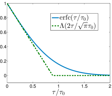
Figure 1: The erfc function and a lower bound using the triangle function $\Lambda$.

III Multimode quantum optical phase estimation

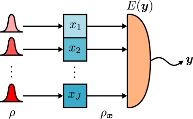
Figure 2: The quantum optical multiparameter phase estimation problem. The initial state $\rho$ may be entangled between the modes, and each mode passes through a phase shift $x_{j}$. The output may be measured via some general joint measurement $E(\boldsymbol{y})$.

We now consider the problem of phase estimation from the measurement of quantum optical modes, as illustrated in Fig. 2. The output quantum state is

$$\rho_{\boldsymbol{x}} =\exp\left(i\boldsymbol{x}^{\top}\hat{\boldsymbol{n}}\right)\rho\exp\left(-i\boldsymbol{x}^{\top}\hat{\boldsymbol{n}}\right),$$ (23)

where $\rho$ is the initial quantum state and $\hat{\boldsymbol{n}}$ is a column vector of photon number operators for the optical modes. We use a hat to distinguish the number operator from other uses of $n$ as an integer. We will not otherwise use a hat to indicate operators. Purifying $\rho_{\boldsymbol{x}}$ to $|\psi(\boldsymbol{x})\rangle$, and taking the purification of $\rho_{\boldsymbol{x}+\boldsymbol{v}\tau}$ to be $\exp\left(i\tau\boldsymbol{v}^{\top}\hat{\boldsymbol{n}}\right)|\psi(\boldsymbol{x})\rangle$, Uhlmann’s theorem Uhlmann (1976) yields a lower bound on $F$ given by Giovannetti et al. (2003)

$$F(\boldsymbol{x},\boldsymbol{x}+\boldsymbol{v}\tau)\geq\left|\left\langle\exp\left(i\tau\boldsymbol{v}^{\top}\hat{\boldsymbol{n}}\right)\right\rangle\right|^{2}$$

$$=\sum_{\boldsymbol{n},\boldsymbol{m}}C(\boldsymbol{n})C(\boldsymbol{m})\cos\left[\tau\boldsymbol{v}^{\top}(\boldsymbol{n}-\boldsymbol{m})\right],$$ (24)

where we have defined $\left\langle O\right\rangle:=\operatorname{tr}\left(O\rho\right)$, and

$$C(\boldsymbol{n}):=\langle\boldsymbol{n}|\rho|\boldsymbol{n}\rangle$$ (25)

is the photon-number distribution of the initial quantum state, with $|\boldsymbol{n}\rangle$ an eigenstate of $\hat{\boldsymbol{n}}$.

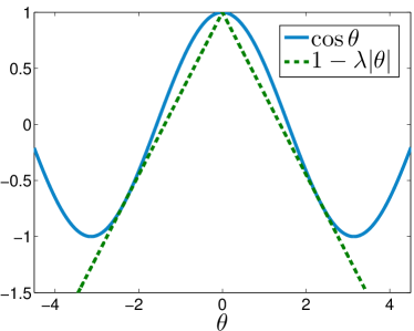
Figure 3: A lower bound on cosine.

To derive a bound on $F(\boldsymbol{x},\boldsymbol{x}+\boldsymbol{v}\tau)$ in terms of the average photon numbers, the following bound on cosine is useful:

$$\cos\theta \geq 1-\lambda|\theta|,$$ (26)

where $\lambda\approx 0.7246$ is a solution of $\lambda(\pi-\arcsin\lambda)=1+\sqrt{1-\lambda^{2}}$, as shown in Fig. 3. This leads to

$$F \geq\sum_{\boldsymbol{n},\boldsymbol{m}}C(\boldsymbol{n})C(\boldsymbol{m})\left[1-\lambda\tau|\boldsymbol{v}^{\top}\left(\boldsymbol{n}-\boldsymbol{m}\right)|\right]$$

$$\geq\sum_{\boldsymbol{n},\boldsymbol{m}}C(\boldsymbol{n})C(\boldsymbol{m})\left[1-\lambda\tau\left(|\boldsymbol{v}^{\top}\boldsymbol{n}|+|\boldsymbol{v}^{\top}\boldsymbol{m}|\right)\right]$$

$$\geq\sum_{\boldsymbol{n},\boldsymbol{m}}C(\boldsymbol{n})C(\boldsymbol{m})\left[1-\lambda\tau\left(|\boldsymbol{v}|^{\top}\boldsymbol{n}+|\boldsymbol{v}|^{\top}\boldsymbol{m}\right)\right]$$

$$=1-2\lambda\tau|\boldsymbol{v}|^{\top}\left\langle\hat{\boldsymbol{n}}\right\rangle,$$ (27)

where $|\boldsymbol{v}|$ means taking the absolute value of each element of $\boldsymbol{v}$. Since $0\leq F\leq 1$, a tighter bound is

$$F \geq\Lambda\left(\frac{\tau}{\tau_{F}}\right), \tau_{F} :=\frac{1}{2\lambda|\boldsymbol{v}|^{\top}\langle\hat{\boldsymbol{n}}\rangle}.$$ (28)

A slightly tighter bound may be obtained using the method in Refs. Giovannetti et al. (2003); Giovannetti and Maccone (2012), but the scaling would remain the same.

Focusing on the mean-square error, putting Eqs. (4), (19), (20), (22), and (28) together, and using $\mathcal{V}\{f(\tau)\}\geq f(\tau)$,

$$\boldsymbol{u}^{\top}\boldsymbol{\Sigma}\boldsymbol{u} \geq\frac{1}{2}\max_{\boldsymbol{v}:\boldsymbol{u}^{\top}\boldsymbol{v}=1}\int_{0}^{\infty}d\tau\,\tau\Lambda\left(\frac{2}{\sqrt{\pi}}\frac{\tau}{\tau_{0}}\right)\Lambda\left(\sqrt{\frac{\tau}{\tau_{F}}}\right)$$

$$=\max_{\boldsymbol{v}:\boldsymbol{u}^{\top}\boldsymbol{v}=1}Z(\boldsymbol{v}),$$ (29)

$$Z(\boldsymbol{v}) :=\left\{\begin{array}[]{ll}\tau_{F}^{2}\left(\frac{1}{20}-\frac{\tau_{F}}{21\sqrt{\pi}\tau_{0}}\right),&\tau_{F}\leq\frac{\sqrt{\pi}\tau_{0}}{2},\\ \frac{\pi\tau_{0}^{2}}{4}\left(\frac{1}{12}-\frac{2}{35}\sqrt{\frac{\sqrt{\pi}\tau_{0}}{2\tau_{F}}}\right),&\tau_{F}>\frac{\sqrt{\pi}\tau_{0}}{2}.\end{array}\right.$$ (32)

The maximization of $Z(\boldsymbol{v})$, subject to the constraint $\boldsymbol{u}^{\top}\boldsymbol{v}=1$, gives the tightest bound, but it is difficult to perform analytically. In the next section, we shall focus on waveform estimation and discover that an appropriate choice of $\boldsymbol{v}$, though suboptimal, can still lead to a reasonably tight bound.

IV Waveform phase estimation

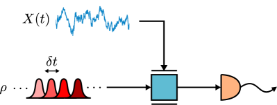
Figure 4: The waveform phase estimation problem.

We now consider phase modulation that varies in time, as illustrated in Fig. 4. Define discrete time as

$$t_{j} =t_{0}+j\delta t,$$ (33)

$j$ being an integer. Each parameter $X_{j}$ corresponds to a phase at time $t_{j}$:

$$X_{j} =X(t_{j}),$$ (34)

and each photon-number operator $\hat{n}_{j}$ is related to the photon-flux operator $I(t_{j})$ by

$$\hat{n}_{j} =I(t_{j})\delta t.$$ (35)

Other quantities are redefined as follows:

$$u_{j} ={u(t_{j})/\delta t}, v_{j} =v(t_{j}),$$ (36)

$$\Sigma_{0jk} =\Sigma_{0}(t_{j},t_{k}), \Sigma_{jk} =\Sigma(t_{j},t_{k}).$$ (37)

In the continuous-time limit $\delta t\to 0$, the mean-square error becomes

$$\boldsymbol{u}^{\top}\boldsymbol{\Sigma}\boldsymbol{u} \to\int_{-\infty}^{\infty}dt\int_{-\infty}^{\infty}dt^{\prime}\,u(t)\Sigma(t,t^{\prime})u(t^{\prime}),$$ (38)

and the constraint in Eq. (29) becomes

$$\boldsymbol{u}^{\top}\boldsymbol{v}=1 \to\int_{-\infty}^{\infty}dt\,u(t)v(t)=1.$$ (39)

To evaluate the bound $Z(\boldsymbol{v})$ given by Eq. (32) in this limit, we need to compute $\tau_{0}$ given by Eq. (21) and $\tau_{F}$ given by Eq. (28). They depend on the following:

$$\boldsymbol{v}^{\top}\boldsymbol{\Sigma}_{0}^{-1}\boldsymbol{v} \to\int_{-\infty}^{\infty}dt\int_{-\infty}^{\infty}dt^{\prime}\,v(t)\Sigma_{0}^{-1}(t,t^{\prime})v(t^{\prime}),$$ (40)

$$|\boldsymbol{v}|^{\top}\langle\hat{\boldsymbol{n}}\rangle \to\int_{-\infty}^{\infty}dt\,|v(t)|\langle I(t)\rangle,$$ (41)

where the continuous-time inverse $\Sigma_{0}^{-1}(t,t^{\prime})$ is defined by

$$\int_{-\infty}^{\infty}dt^{\prime}\,\Sigma_{0}(t,t^{\prime})\Sigma_{0}^{-1}(t^{\prime},t^{\prime\prime}) =\delta(t-t^{\prime\prime}).$$ (42)

Assume now that the prior statistics of $X(t)$ are stationary. This means that we can define a prior power spectral density $\tilde{\Sigma}_{0}(\omega)$ such that

$$\Sigma_{0}(t,t^{\prime}) =\int_{-\infty}^{\infty}\frac{d\omega}{2\pi}\tilde{\Sigma}_{0}(\omega)\exp[i\omega(t-t^{\prime})],$$ (43)

and the inverse of $\Sigma_{0}$ is given by

$$\Sigma_{0}^{-1}(t,t^{\prime}) =\int_{-\infty}^{\infty}\frac{d\omega}{2\pi}\frac{1}{\tilde{\Sigma}_{0}(\omega)}\exp[i\omega(t-t^{\prime})].$$ (44)

We then obtain

$$\boldsymbol{v}^{\top}\boldsymbol{\Sigma}_{0}^{-1}\boldsymbol{v} \to\int_{-\infty}^{\infty}\frac{d\omega}{2\pi}\frac{|\tilde{v}(\omega)|^{2}}{\tilde{\Sigma}_{0}(\omega)},$$ (45)

$$\tilde{v}(\omega) :=\int_{-\infty}^{\infty}dt\,v(t)\exp(-i\omega t).$$ (46)

We are particularly interested in the estimation error at a particular time $t_{0}$, in which case $u(t)=\delta(t-t_{0})$ and from Eq. (39), $v(t_{0})=1$. We will see below that the choice $\tilde{v}(\omega)=e^{i\omega t_{0}}2\pi T\Lambda(T\omega)$, so

$$v(t) =\operatorname{sinc}^{2}\left(\frac{t-t_{0}}{2T}\right),$$ (47)

where

$$\operatorname{sinc}x :=\left\{\begin{array}[]{ll}(\sin x)/x,&x\neq 0,\\ 1,&x=0,\end{array}\right.$$ (50)

is a convenient one for deriving a lower bound, for a suitable choice of characteristic time $T$. It gives

$$|\boldsymbol{v}|^{\top}\left\langle\hat{\boldsymbol{n}}\right\rangle \to\int_{-\infty}^{\infty}dt\,|v(t)|\left\langle I(t)\right\rangle=2\pi T\mathcal{N}(t_{0}),$$ (51)

where we have defined a weighted average of the flux around $t_{0}$ by

$$\mathcal{N}(t_{0}):=\frac{\int_{-\infty}^{\infty}dt\,|v(t)|\left\langle I(t)\right\rangle}{\int_{-\infty}^{\infty}dt\,|v(t)|}.$$ (52)

We wish to consider $\tilde{\Sigma}_{0}(\omega)$ to be a spectrum with power-law scaling as $\kappa^{p-1}/|\omega|^{p}$ for $\omega$ large. This scaling is problematic for small $\omega$, because it diverges at $\omega=0$. To avoid this divergence, we assume Van Trees (2001)

$$\tilde{\Sigma}_{0}(\omega) =\frac{\kappa^{p-1}}{|\omega|^{p}+\gamma^{p}},$$ (53)

for some constant $\gamma$. For example, $p=2$ gives the Ornstein-Uhlenbeck process used in Refs. Wheatley et al. (2010); Yonezawa et al. (2012). The integral in Eq. (45) can then be computed analytically, resulting in

$$\boldsymbol{v}^{\top}\boldsymbol{\Sigma}_{0}^{-1}\boldsymbol{v} \to\frac{8\pi}{p_{3}\kappa^{p-1}T^{p-1}}+\frac{4\pi\gamma^{p}T}{3\kappa^{p-1}}\approx\frac{8\pi}{p_{3}\kappa^{p-1}T^{p-1}},$$

$$p_{3} :=(p+1)(p+2)(p+3),$$ (54)

where the approximation assumes

$$\gamma T\ll\left(\frac{6}{p_{3}}\right)^{1/p},$$ (55)

which will be justified later. Under this approximation, we will find a bound on the mean-square error that is independent of $\gamma$. Alternative choices for removing the singularity at $\omega=0$ yield similar results, (see Appendix A). That is, Eq. (54) depends on the scaling of the spectrum for large $\omega$, not on the behavior for small $\omega$.

The largest $Z(\boldsymbol{v})$ in Eq. (32) is obtained by setting

$$\tau_{F} =\frac{\sqrt{\pi}}{2}\tau_{0}.$$ (56)

Using Eqs. (54) and (51), and recalling the definitions of $\tau_{0}$ and $\tau_{F}$ from (21) and (28), respectively, we get

$$T =\left[\frac{1}{4\pi^{2}\lambda^{2}p_{3}\kappa^{p-1}\mathcal{N}^{2}(t_{0})}\right]^{1/(p+1)}.$$ (57)

Equation (55) can then be justified in the asymptotic high $\mathcal{N}$ limit, because $T$ becomes arbitrarily small. The quantum bound in Eq. (29) becomes

$$\Sigma(t_{0},t_{0}) \geq\frac{11}{420}\left(\frac{p_{3}}{4}\right)^{2/(p+1)}\left[\frac{\kappa}{4\pi\lambda\mathcal{N}(t_{0})}\right]^{2(p-1)/(p+1)}.$$ (58)

Rather than considering the error at a single time, we wish to bound the error averaged over time. This means bounding

$$\bar{\Sigma}:=\lim_{T_{\max}\to\infty}\frac{1}{2T_{\max}}\int_{-T_{\max}}^{T_{\max}}dt_{0}\,\Sigma(t_{0},t_{0}),$$ (59)

in terms of the time-averaged flux,

$$\mathcal{N}:=\lim_{T_{\max}\to\infty}\frac{1}{2T_{\max}}\int_{-T_{\max}}^{T_{\max}}dt_{0}\left\langle I(t_{0})\right\rangle.$$ (60)

It is easy to see that the average of $\mathcal{N}(t_{0})$ is equal to $\mathcal{N}$. Next, because $1/x^{2(p-1)/(p+1)}$ is a convex function (for $p>1$), the time average of $1/[\mathcal{N}(t_{0})]^{2(p-1)/(p+1)}$ is lower-bounded by $1/\mathcal{N}^{2(p-1)/(p+1)}$ using Jensen’s inequality. As a result, we obtain the final result

$$\bar{\Sigma} \geq c_{Z}\left(\frac{\kappa}{\mathcal{N}}\right)^{2(p-1)/(p+1)},$$ (61)

where $c_{Z}$ is the dimensionless constant

$$c_{Z} =\frac{11}{420}\left(\frac{p_{3}}{4}\right)^{2/(p+1)}\left(\frac{1}{4\pi\lambda}\right)^{2(p-1)/(p+1)}.$$ (62)

That is, we have a lower bound on the time-averaged mean-square error in terms of the time-averaged flux. The $(\kappa/\mathcal{N})^{2(p-1)/(p+1)}$ scaling was previously proposed in Ref. Berry et al. (2013) as the Heisenberg limit for a stochastically varying phase with a power-law spectrum. However, the proof in that work applies only to a specific class of Gaussian quantum states. Here, we have proved the scaling for arbitrary quantum states by introducing the powerful new technique of the quantum Bell-Ziv-Zakai bound.

V Achieving the optimal scaling

A lower bound is not a Heisenberg limit, and is indeed of limited value at all, if it is not close to a realizable error. Here we demonstrate that the scaling in Eq. (61) is indeed achievable in principle. Consider an estimation strategy where the probe field is concentrated into pulses separated by time $T$, as shown in Fig. 5. Each pulse is assumed to be so short that the phase $X(t)$ does not vary during the pulse duration. The value that we select for $T$ here will be slightly different than in the previous section, but the scaling is the same. With average flux $\mathcal{N}$, each pulse can have an average photon number of ${\cal N}T$.

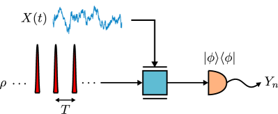
Figure 5: A pulsed phase measurement scheme to achieve the optimal scaling.

We first assume that the phase modulation is weak; viz.,

$$\mathbb{E}\left[X^{2}(t)\right] \ll 1.$$ (63)

Using canonical phase measurements and minimum-uncertainty states within each pulse, the observation $Y_{n}\in(-\pi,\pi]$ at each sampling can be linearized as

$$Y_{n} \approx X(nT)+\xi_{n},$$ (64)

where the moments of the noise random variable $\xi_{n}$ are

$$\mathbb{E}\left(\xi_{n}|X\right)\approx 0,\quad\mathbb{E}\left(\xi_{n}\xi_{m}|X\right)\approx\delta_{nm}\frac{(4/27)|z_{A}|^{3}}{(\mathcal{N}T)^{2}},$$ (65)

with $z_{A}$ being the first negative root of the Airy function Bandilla et al. (1991). The above moments are exact in the asymptotic limit of large ${\cal N}T$.

The condition given by Eq. (63) can be relaxed for large phase fluctuations by making the canonical phase measurements adaptive Wiseman (1995), as shown in Appendix B. A rigorous accounting of the error due to phase ambiguity will be presented in Sec. VII in the case of a periodic distortion function. For the remainder of this section we will assume Eqs. (63)–(65) for simplicity.

After all measurements are made, the final estimates can be constructed via the Whittaker-Shannon interpolation formula:

$$\check{X}(t) :=\sum_{n=-\infty}^{\infty}Y_{n}\operatorname{sinc}\left(\frac{\pi t}{T}-\pi n\right)$$

$$=X_{T}(t)+\xi(t),$$ (66)

$$X_{T}(t) :=\sum_{n=-\infty}^{\infty}X(nT)\operatorname{sinc}\left(\frac{\pi t}{T}-\pi n\right),$$ (67)

$$\xi(t) :=\sum_{n=-\infty}^{\infty}\xi_{n}\operatorname{sinc}\left(\frac{\pi t}{T}-\pi n\right).$$ (68)

We use this suboptimal interpolation formula rather than optimal estimation because the error is easier to evaluate. The mean-square error becomes

$$\mathbb{E}\left[\check{X}(t)-X(t)\right]^{2} =\mathbb{E}\left[\xi(t)+X_{T}(t)-X(t)\right]^{2}$$

$$=\mathbb{E}\left[\xi^{2}(t)\right]+\mathbb{E}\left[X_{T}(t)-X(t)\right]^{2},$$ (69)

which consists of an aliasing error and a measurement error. Here we have used the relation

$$\mathbb{E}\left\{\xi(t)\left[X_{T}(t)-X(t)\right]\right\} =0.$$ (70)

Averaging over time (see Appendix C), the aliasing error is

$$\frac{1}{T}\int_{0}^{T}dt\,\mathbb{E}\left[X_{T}(t)-X(t)\right]^{2} =\frac{2}{\pi}\int_{\pi/T}^{\infty}d\omega\,\tilde{\Sigma}_{0}(\omega)$$

$$\approx\frac{2(\kappa T)^{p-1}}{\pi^{p}(p-1)},$$ (71)

which assumes

$$\gamma T\ll\pi,$$ (72)

to be justified later, and the measurement error is

$$\frac{1}{T}\int_{0}^{T}dt\,\mathbb{E}\left[\xi^{2}(t)\right]\approx\frac{(4/27)|z_{A}|^{3}}{({\cal N}T)^{2}}$$ (73)

via Eq. (65). The overall error is hence

$$\bar{\Sigma}\approx\frac{2\left(\kappa T\right)^{p-1}}{\pi^{p}(p-1)}+\frac{(4/27)|z_{A}|^{3}}{({\cal N}T)^{2}}.$$ (74)

Note that the first term increases with $T$, whereas the second term decreases with $T$. This is as we expect, because increasing $T$ means that the phase is sampled less frequently and can vary more in between samples, but also means that more power is available to estimate each sample, which reduces the error.

The optimal value of $T$ is

$$T=\left(\frac{(4/27)|z_{A}|^{3}\pi^{p}}{{\cal N}^{2}\kappa^{p-1}}\right)^{1/(p+1)},$$ (75)

which justifies the assumption in Eq. (72) in the asymptotic high $\mathcal{N}$ limit and yields an average variance of

$$\bar{\Sigma} \approx c_{A}(\kappa/{\cal N})^{2(p-1)/(p+1)},$$ (76)

where $c_{A}>c_{Z}$ is the dimensionless constant

$$c_{A} =\frac{p+1}{p-1}\left(4|z_{A}|^{3}/27\right)^{(p-1)/(p+1)}\pi^{-2p/(p+1)}.$$ (77)

Thus the achievable variance has the same scaling with respect to $\kappa/\cal N$ as that in the lower bound in Eq. (61), but with a larger multiplicative coefficient. This demonstrates that the scaling of the lower bound is tight, and represents a rigorous Heisenberg limit.

VI Periodic distortion functions

Above we have considered phase estimation as an example of the application of the quantum Bell-Ziv-Zakai bounds. Phase measurements are intrinsically modulo $2\pi$, because they are unable to distinguish between phases that differ by multiples of $2\pi$. For this reason, phase will typically be taken to be in some standard region, such as $(-\pi,\pi]$. Then a phase of $-\pi+\delta_{1}$, for some small $\delta_{1}>0$, can easily be estimated as $\pi-\delta_{2}$, for some $\delta_{2}>0$. It seems unrealistic to quantify the error as $\approx 2\pi$, because the phase difference is small modulo $2\pi$. For this reason it is better to use periodic distortion functions for measurements of this type.

In the notation of Ref. Basu and Bresler (2000), which we now adopt, the distortion function is a vector $\boldsymbol{D}$ with components for each of the parameters $x_{j}$ to be measured. For the distortion function to be periodic, it should satisfy

$$D_{j}(\epsilon_{j}+2\pi m_{j})=D_{j}(\epsilon_{j}),$$ (78)

for any vector of integers $\boldsymbol{m}$. The distortion function should satisfy most of the conditions used before. It should be symmetric, have $D_{j}(0)=0$, and be differentiable and nondecreasing on $[0,\pi)$. A further condition is that

$$\dot{D}_{j}(\epsilon_{j})\leq\dot{D}_{j}(\pi-\epsilon_{j}),$$ (79)

for $\pi/2+2\pi m_{j}\leq\epsilon_{j}\leq\pi+2\pi m_{j}$. This condition is a technical condition needed for the results of Ref. Basu and Bresler (2000). An example of a periodic distortion function satisfying these conditions is the periodic modification of the mean-square error,

$$D_{j}(\epsilon_{j})=([\epsilon_{j}]_{2\pi})^{2},$$ (80)

where the notation

$$[\epsilon]_{2\pi}:=\epsilon+2\pi\operatorname{floor}\left(\frac{1}{2}-\frac{\epsilon}{2\pi}\right)$$ (81)

denotes the value of $\epsilon$ modulo the interval $(-\pi,\pi]$, as shown in Fig. 6.

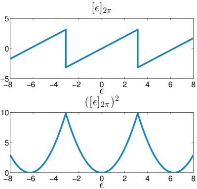
Figure 6: Top: the modulo function $[\epsilon]_{2\pi}$. Bottom: square of the modulo function.

Using these conditions, it can be shown that (see Eq. (15) of Basu and Bresler (2000))

$$\mathbb{E}\left[D_{j}(|\epsilon_{j}|)\right]=\frac{1}{2}\int_{0}^{2\pi}d\tau\,\dot{D}_{j}\left(\frac{\tau}{2}\right)\textrm{Pr}\left(|[\epsilon_{j}]_{2\pi}|\geq\frac{\tau}{2}\right).$$ (82)

Note the similarity between this expression for the periodic case and Eq. (3) for the non-periodic case. This expression then gives (see Eq. (19) of Basu and Bresler (2000))

$$\mathbb{E}\left[D_{j}(|\epsilon_{j}|)\right]\geq\frac{1}{2}\int_{0}^{\pi}d\tau\,\dot{D}_{j}\left(\frac{\tau}{2}\right)\max_{\boldsymbol{v}:v_{j}=1}\int_{-\pi}^{\pi}d\boldsymbol{x}\,[P_{\boldsymbol{X}}(\boldsymbol{x})$$

$$\quad+P_{\boldsymbol{X}}([\boldsymbol{x}+\boldsymbol{v}\tau]_{2\pi})]P_{e}(\boldsymbol{x},[\boldsymbol{x}+\boldsymbol{v}\tau]_{2\pi}),$$ (83)

where the bounds on the integral indicate the bounds for each component of $\boldsymbol{x}$.

It is easily seen that Property 1 of Bell et al. (1997) holds in the periodic case as well, which gives

$$\mathbb{E}\left[D_{j}(|\epsilon_{j}|)\right]\geq\frac{1}{2}\int_{0}^{\pi}d\tau\,\dot{D}_{j}\left(\frac{\tau}{2}\right)\max_{\boldsymbol{v}:v_{j}=1}\int_{-\pi}^{\pi}d\boldsymbol{x}\,\min(P_{\boldsymbol{X}}(\boldsymbol{x}),$$

$$\quad P_{\boldsymbol{X}}([\boldsymbol{x}+\boldsymbol{v}\tau]_{2\pi}))P_{e}^{\rm el}(\boldsymbol{x},[\boldsymbol{x}+\boldsymbol{v}\tau]_{2\pi})$$ (84)

Next, using Eq. (13), for the case of quantum measurements we obtain

$$\mathbb{E}\left[D_{j}(|\epsilon_{j}|)\right]\geq{} \frac{1}{2}\int_{0}^{\pi}d\tau\,\dot{D}_{j}\left(\frac{\tau}{2}\right)\max_{\boldsymbol{v}:v_{j}=1}\int_{-\pi}^{\pi}d\boldsymbol{x}$$

$$\times\min[P_{\boldsymbol{X}}(\boldsymbol{x}),P_{\boldsymbol{X}}([\boldsymbol{x}+\boldsymbol{v}\tau]_{2\pi})]$$

$$\times\left[1-\sqrt{1-F(\boldsymbol{x},\boldsymbol{x}+\boldsymbol{v}\tau)}\right].$$ (85)

Note that $[\bullet]_{2\pi}$ is not needed in the fidelity, because the state is also periodic modulo $2\pi$.

To provide a result for Gaussian variation of $\boldsymbol{x}$ we then encounter a problem. Gaussian distributions always extend from $-\infty$ to $+\infty$ (even though they exponentially decay), whereas the variation of $x_{j}$ is limited to the interval $(-\pi,\pi]$. Instead the method we use is to take a Gaussian probability distribution $P_{G}$, and wrap it around $2\pi$. This would physically correspond to a case where a phase shift is caused by variation in an unbounded quantity (such as the position of a mirror on which the beam is incident Iwasawa et al. (2013)), that has Gaussian statistics. The probability would then be given by

$$P_{\boldsymbol{X}}(\boldsymbol{x})=\sum_{\boldsymbol{n}}P_{G}(\boldsymbol{x}+2\pi\boldsymbol{n}),$$ (86)

where the sum is over all vectors of integers, $\boldsymbol{n}$. Next, the integral over $\boldsymbol{x}$ in Eq. (VI) can be lower bounded as

$$\int_{-\pi}^{\pi}d\boldsymbol{x}\min\left[P_{\boldsymbol{X}}(\boldsymbol{x}),P_{\boldsymbol{X}}([\boldsymbol{x}+\boldsymbol{v}\tau]_{2\pi})\right]$$

$$=\int_{-\pi}^{\pi}d\boldsymbol{x}\min\left[\sum_{\boldsymbol{n}}P_{G}(\boldsymbol{x}+2\pi\boldsymbol{n}),\right.$$

$$\left.\hskip 100.00015pt\sum_{\boldsymbol{m}}P_{G}(\boldsymbol{x}+2\pi\boldsymbol{m}+\boldsymbol{v}\tau)\right]$$

$$\geq\int_{-\pi}^{\pi}d\boldsymbol{x}\sum_{\boldsymbol{n}}\min\left[P_{G}(\boldsymbol{x}+2\pi\boldsymbol{n}),P_{G}(\boldsymbol{x}+2\pi\boldsymbol{n}+\boldsymbol{v}\tau)\right]$$

$$=\int_{-\infty}^{\infty}d\boldsymbol{x}\min\left[P_{G}(\boldsymbol{x}),P_{G}(\boldsymbol{x}+\boldsymbol{v}\tau)\right].$$ (87)

We therefore obtain a result closely analogous to Eq. (19):

$$\mathbb{E}\left[D_{j}(|\epsilon_{j}|)\right] \geq\frac{1}{2}\int_{0}^{\pi}d\tau\,\dot{D}_{j}\left(\frac{\tau}{2}\right)$$

$$\quad\times\max_{\boldsymbol{v}:v_{j}=1}\int d\boldsymbol{x}\,\min[P_{G}(\boldsymbol{x}),P_{G}(\boldsymbol{x}+\boldsymbol{v}\tau)]$$

$$\quad\times\left[1-\sqrt{1-F(\boldsymbol{x},\boldsymbol{x}+\boldsymbol{v}\tau)}\right],$$ (88)

where the second integral is over all $\boldsymbol{x}$. On the right-hand side, the main differences between this expression and that in Eq. (19) are that the integral is up to $\tau=\pi$, rather than $\tau\to\infty$, and the valley-filling function $\mathcal{V}$ is not applied here.

Again considering mean-square error for quantum optical phase, Eq. (29) is modified to

$$\mathbb{E}\left[D_{j}(|\epsilon_{j}|)\right] \geq\frac{1}{2}\max_{\boldsymbol{v}:v_{j}=1}\int_{0}^{\pi}d\tau\,\tau\Lambda\left(\frac{2}{\sqrt{\pi}}\frac{\tau}{\tau_{0}}\right)\Lambda\left(\sqrt{\frac{\tau}{\tau_{F}}}\right)$$

$$=\max_{\boldsymbol{v}:v_{j}=1}Z_{\pi}(\boldsymbol{v}),$$ (89)

where

$$Z_{\pi}(\boldsymbol{v}):=$$

$$\left\{\begin{array}[]{ll}\tau_{F}^{2}\left(\frac{1}{20}-\frac{\tau_{F}}{21\sqrt{\pi}\tau_{0}}\right),&\pi\geq\tau_{F}\leq\frac{\sqrt{\pi}\tau_{0}}{2},\\ \frac{\pi\tau_{0}^{2}}{4}\left(\frac{1}{12}-\frac{2}{35}\sqrt{\frac{\sqrt{\pi}\tau_{0}}{2\tau_{F}}}\right),&\tau_{F}>\frac{\sqrt{\pi}\tau_{0}}{2}\leq\pi,\\ \pi^{2}\left(\frac{1}{4}-\frac{\sqrt{\pi}}{3\tau_{0}}-\frac{\sqrt{\pi}}{5\sqrt{\tau_{F}}}+\frac{2\pi}{7\tau_{0}\sqrt{\tau_{F}}}\right),&\tau_{F}>\pi<\frac{\sqrt{\pi}\tau_{0}}{2}.\end{array}\right.$$ (93)

The key fact to notice about $Z_{\pi}$ is that it corresponds to $Z$ when either of $\tau_{0}$ or $\tau_{F}$ is small. In the analysis in Sec. IV we took parameters such that both $\tau_{0}$ or $\tau_{F}$ are small for large ${\cal N}/\kappa$ (which is the limit we are considering). Therefore the difference between $F_{\pi}$ and $F$ has no effect on the bound for the measurements.

The only other difference is that the left-hand side in Eq. (89) is the mean-square error, whereas the left-hand side in Eq. (29) contains the full covariance matrix. That is, Eq. (89) corresponds to taking $u_{\ell}=\delta_{\ell,j}$, to give the mean-square error for $x_{j}$. However, this is exactly what is used in Sec. IV. Hence the analysis in Sec. IV continues to hold, and Eq. (61) is also a lower bound when the mean-square error modulo $2\pi$ is used.

VII Achieving the optimal scaling: effect of phase ambiguity

The analysis of the technique for achieving the optimal scaling given in Sec. V does not fully address the fact that the phase can only be measured modulo $2\pi$. When tracking a phase, it is possible to resolve this ambiguity from the fact that the variation of the phase is continuous. Provided the phase does not change too much between successive estimates, and each estimate is reasonably accurate, changes by $2\pi$ can be kept track of. That is, one can add suitable multiples of $2\pi$ to $Y_{n}$ to give $\check{X}_{n}$, such that $|\check{X}_{n}-\check{X}_{n-1}|\leq\pi$. If the initial range of the phase is known, then the error should not exceed $\pi$.

This approach is problematic when the phase can vary arbitrarily far from zero, such as for a Wiener process. There is a non-zero possibility, however small, of choosing the wrong interval at any step, and from that point on there will continue to be an error of size $2\pi$ due to this initial error. This is called a phase-wrap error. When averaging measurements over an arbitrarily long period of time, the phase error can grow to be arbitrarily large. For the phase variation we consider, the Fourier spectrum $\tilde{\Sigma}_{0}(\omega)$ is bounded for $\omega=0$, so the prior distribution has a bounded variance for any given time. This means that the error due to phase-wraps is not unbounded, but it is still problematic.

Here we consider the periodic distortion function, given by the mean-square error modulo $2\pi$. In this case phase-wrap errors for individual points on their own do not matter, because they do not increase a periodic distortion function. The problem appears when we consider estimation of the phase between the sample points, where the phase is interpolated. The estimated interpolation error for the Whittaker-Shannon interpolation formula is only accurate if there are no phase-wrap errors.

To simplify the problem, we take $X(t)$ to vary over the entire real line. Since the error is quantified modulo $2\pi$, the estimation problem is identical to that where $X(t)$ is limited to the region $(-\pi,\pi]$. There is the additional advantage that the probability distribution is now exactly Gaussian, rather than given by Eq. (86).

To address the effect of phase-wrap errors on the interpolation, we specify that we consider the mean-square deviation between the interpolated estimate and the actual phase at a given time $t$. We regard the phase estimate $\check{X}_{n_{t}}$ for the sample time nearest $t$ to be in the interval $(-\pi,\pi]$. This means that the difference between $\check{X}_{n_{t}}$ and $X(n_{t}T)$ will (approximately) be $2\pi K$ for some integer $K$, the number of phase wrappings there are between $\check{X}_{n}$ and $X(nT)$. In itself, this difference is unimportant if deviations are only measured modulo $2\pi$. What is important is that this difference is maintained for the other estimates. To achieve this, for all other phase estimates $\check{X}_{n}$, we add or subtract multiples of $2\pi$ as needed to make the differences between neighboring estimates no more than $\pi$; in particular, $\check{X}_{n}-\check{X}_{n-1}\in(-\pi,\pi]$. Provided certain conditions are met (discussed below), the difference between $\check{X}_{n}$ and $X(nT)$ will be close to $2\pi K$ for all $n$; that is, the same multiple of $2\pi$. When there are phase-wrap errors, so the difference is close to $2\pi K_{n}$ where $K_{n}$ is dependent on $n$, this will introduce error to the interpolation, but this error can be bounded.

Now we make this discussion more rigorous. First, the noise random variable $\xi_{n}$ is redefined as

$$\xi_{n}:=[Y_{n}-X(nT)]_{2\pi}.$$ (94)

With this definition, the moments given in Eq. (65) are correct. We can give $\check{X}_{n}$ as

$$\check{X}_{n}=X(nT)+\xi_{n}+2\pi K_{n},$$ (95)

Recall that $Y_{n}$ is the measurement result in the interval $(-\pi,\pi]$, which is then adjusted to $\check{X}_{n}$ by adding or subtracting multiples of $2\pi$.

The interpolated values $\check{X}(t)$ can be expressed as

$$\check{X}(t)=X_{T}(t)+\xi(t)+2\pi K(t),$$ (96)

where $X_{T}(t)$ and $\xi(t)$ are defined as in Eqs. (67) and (68), and

$$K(t):=\sum_{n=-\infty}^{\infty}K_{n}\operatorname{sinc}\left(\frac{\pi t}{T}-\pi n\right).$$ (97)

This shows why we want the difference between the estimates and values to remain the same multiple of $2\pi$. If they do, then $K(t)$ simply becomes the constant $K$. On the other hand, if $K_{n}$ varies with $n$, then $K(t)$ will not be an integer, and the extra term $2\pi K(t)$ in Eq. (96) will give an increased error modulo $2\pi$.

The analysis of the error in Eq. (V) needs to be performed modulo $2\pi$. First, define

$$\Delta(t):=[\xi(t)+X_{T}(t)-X(t)]_{2\pi}.$$ (98)

In terms of this quantity we obtain

$$\mathbb{E}\left[[\check{X}(t)-X(t)]_{2\pi}^{2}\right]=\mathbb{E}\left[\left[2\pi K(t)+\Delta(t)\right]_{2\pi}^{2}\right]$$

$$\leq\mathbb{E}\left[\left\{[2\pi K(t)]_{2\pi}+\Delta(t)\right\}^{2}\right]$$

$$=\mathbb{E}\left[[2\pi K(t)]_{2\pi}^{2})\right]+\mathbb{E}\left[\Delta^{2}(t)\right]+2\mathbb{E}\left[\Delta(t)[2\pi K(t)]_{2\pi}\right]$$

$$\leq\left\{\sqrt{\mathbb{E}\left[[2\pi K(t)]_{2\pi}^{2}\right]}+\sqrt{\mathbb{E}\left[\Delta^{2}(t)\right]}\right\}^{2}.$$ (99)

The time-averaged value of $\mathbb{E}\left[\Delta^{2}(t)\right]$ is exactly what was obtained as in Sec. V, with the result given in Eq. (74). Note also that we can upper bound the time-averaged value of $\mathbb{E}\left[[\check{X}(t)-X(t)]_{2\pi}^{2}\right]$ using the time averaged values of $\mathbb{E}\left[\Delta^{2}(t)\right]$ and $\mathbb{E}\left[[2\pi K(t)]_{2\pi}^{2}\right]$. That is because $\mathbb{E}\left[[\check{X}(t)-x(t)]_{2\pi}^{2}\right]$ is a concave function of these quantities. The remaining task is therefore to find the time-averaged value of $\mathbb{E}\left[[2\pi K(t)]_{2\pi}^{2}\right]$.

To achieve this, we need to bound the probabilities of phase-wrap errors. If $t$ is a sample time so $t=n_{t}T$, then $K(t)=K_{n}$, and $[2\pi K(t)]_{2\pi}$ is equal to zero. Therefore, in the remainder of this discussion, we will assume that $t$ is not a sample time. Let $L_{n}$ be the multiple of $2\pi$ that we have added to the measurement result $Y_{n}$ to give $\check{X}_{n}$; that is

$$\check{X}_{n}=Y_{n}+2\pi L_{n}.$$ (100)

We wish to consider the error in interpolating at the given time $t$. Without loss of generality, this time can be taken to be in the interval $(0,T/2]$. This is because there is translation symmetry and time-reversal symmetry. One can simply translate the time by a multiple of $T$, and change the sample numbering such that $n=0$ or $n=1$ corresponds to the closest sample time. That would yield $t\in(0,T)$. Then, if $t\in(T/2,T)$, one can simply reverse all times about $T/2$, so $t\in(0,T/2]$.

We can select $n_{t}={\rm round}(t/T)$ with the “round half down” convention, so if $t$ is equidistant between two sample times, we take the smaller sample time. In that case, for $t\in(0,T/2]$, $n_{t}=0$. We are then starting with $\check{X}_{0}$ taken to be in the interval $(-\pi,\pi]$, so $\check{X}_{0}=Y_{0}$ and $L_{0}=0$. Then all other values of $L_{n}$ are selected such that $|\check{X}_{n+1}-\check{X}_{n}|\leq\pi$. The goal of this is to ensure that the values of $K_{n}$ are equal (or at least close) to $K_{0}$. Using Eqs. (95) and (100), we obtain

$$2\pi|K_{n+1}-K_{n}|$$

$$=|\check{X}_{n+1}-\check{X}_{n}+\xi_{n}-\xi_{n+1}+X(nT)-X((n+1)T)|$$

$$\leq|\check{X}_{n+1}-\check{X}_{n}|+|\xi_{n}-\xi_{n+1}|+|X(nT)-X((n+1)T)|$$

$$\leq\pi+|\xi_{n}-\xi_{n+1}|+|X(nT)-X((n+1)T)|.$$ (101)

In the last line we have used the fact that the values of $L_{n}$ have been chosen such that $|\check{X}_{n+1}-\check{X}_{n}|\leq\pi$. Now, if it is the case that $|\xi_{n}-\xi_{n+1}|+|X(nT)-X((n+1)T)|$ is less than $\pi$, then $2\pi|K_{n+1}-K_{n}|<2\pi$. Because $K_{n}$ takes integer values, this inequality implies that $K_{n+1}=K_{n}$.

In the following, we will wish to ensure that $|\xi_{n}-\xi_{n+1}|<\pi/2$, and $|X(nT)-X((n+1)T)|<\pi/2$. Note that $|\xi_{n}|\leq\pi$, so we must always obtain $|\xi_{n}-\xi_{n+1}|\leq 2\pi$. Below we will show that the probability of $|X(nT)-X((n+1)T)|\geq\pi/2$ is negligible. Given that $|X(nT)-X((n+1)T)|<\pi/2$ and $|\xi_{n}-\xi_{n+1}|\leq 2\pi$, we must have $2\pi|K_{n+1}-K_{n}|<4\pi$. This ensures that $K_{n}$ cannot change by more than $1$; that is, we do not have more than $1$ phase-wrap error at a time.

To consider the effect of a phase-wrap error, let $Z_{n}:=K_{n}-K_{n-1}$, which can take values $Z_{n}\in\{0,-1,+1\}$ with non-negligible probability (since the probability of multiple phase-wrap errors is insignificant). Then we obtain, for positive $n$,

$$K_{n}=K_{0}+\sum_{m=1}^{n}Z_{m}.$$ (102)

Similarly, for negative $n$,

$$K_{n}=K_{0}-\sum_{m=n+1}^{0}Z_{m}.$$ (103)

Therefore we can write $K(t)$ as

$$K(t) =K_{0}+\sum_{n=1}^{\infty}\sum_{m=1}^{n}Z_{m}\operatorname{sinc}\left(\frac{\pi t}{T}-\pi n\right)$$

$$\quad+\sum_{n=-\infty}^{-1}\sum_{m=n+1}^{0}Z_{m}\operatorname{sinc}\left(\frac{\pi t}{T}-\pi n\right)$$

$$=K_{0}+\sum_{m=1}^{\infty}Z_{m}\sum_{n=m}^{\infty}\operatorname{sinc}\left(\frac{\pi t}{T}-\pi n\right)$$

$$\quad+\sum_{m=-\infty}^{0}Z_{m}\sum_{n=-\infty}^{m-1}\operatorname{sinc}\left(\frac{\pi t}{T}-\pi n\right)$$

$$=K_{0}+\frac{1}{2\pi}\sum_{m=-\infty}^{\infty}Z_{m}a_{m},$$ (104)

where (see Appendix D)

$$a_{m}:=(-1)^{m}\sin\left(\frac{\pi t}{T}\right)$$

$$\times\begin{cases}\psi\left(\frac{m}{2}-\frac{t}{2T}\right)-\psi\left(\frac{1}{2}+\frac{m}{2}-\frac{t}{2T}\right),&m>0\\ \psi\left(\frac{1}{2}-\frac{m}{2}+\frac{t}{2T}\right)-\psi\left(1-\frac{m}{2}+\frac{t}{2T}\right),&m\leq 0,\end{cases}$$ (105)

where $\psi$ is the digamma function $\psi(x)=\Gamma^{\prime}(x)/\Gamma(x)$.

Due to symmetry, $\mathbb{E}\left[Z_{m}\right]=0$. Also, note that $\mathbb{E}\left[Z_{n}Z_{m}\right]\approx 0$ for $|n-m|>1$. This is because the errors in the phase estimates are independent, so the probability of $|\xi_{n}-\xi_{n+1}|$ exceeding $\pi/2$ is independent of the probability of $|\xi_{m}-\xi_{m+1}|$ exceeding $\pi/2$. This means that the only way that $Z_{n}$ can be correlated with $Z_{m}$ is through correlations in the variation of $X$. That is, the probability of $|X(nT)-X((n+1)T)|$ exceeding $\pi/2$ is correlated with that for $|X(mT)-X((m+1)T)|$. However, because the probability for this is negligible, the overall correlations are negligible. For a rigorous proof that $\mathbb{E}\left[Z_{n}Z_{m}\right]$ can be neglected, see Appendix F.

As a result, we can bound $\mathbb{E}\left[[2\pi K(t)]_{2\pi}^{2}\right]$ as follows:

$$\mathbb{E}\left[[2\pi K(t)]_{2\pi}^{2}\right]$$

$$=\mathbb{E}\left[[2\pi(K(t)-K_{0})]_{2\pi}^{2}\right]$$

$$\leq\mathbb{E}\left[[2\pi(K(t)-K_{0})]^{2}\right]$$

$$=\mathbb{E}\left[\left(\sum_{m=-\infty}^{\infty}Z_{m}a_{m}\right)^{2}\right]$$

$$\approx\sum_{m=-\infty}^{\infty}\mathbb{E}\left[Z_{m}^{2}\right]a_{m}^{2}+2\sum_{m=-\infty}^{\infty}\mathbb{E}\left[Z_{m}Z_{m+1}\right]a_{m}a_{m+1}$$

$$\mathrel{\raise 2.58334pt\hbox{$<$}\kern-7.7778pt\lower 2.79857pt\hbox{$\sim$}}p_{\rm err}\left[\sum_{m=-\infty}^{\infty}a_{m}^{2}+2\sum_{m=-\infty}^{\infty}|a_{m}a_{m+1}|\right],$$ (106)

where $\mathrel{\raise 2.58334pt\hbox{$<$}\kern-7.7778pt\lower 2.79857pt\hbox{$\sim$}}$ indicates that terms exponentially small in ${\cal N}/\kappa$ have been omitted, and $p_{\rm err}$ is the probability of a phase wrap error at each step. Because $Z_{m}$ is limited to $\{0,-1,+1\}$ with high probability, $\mathbb{E}\left[Z_{m}^{2}\right]\approx p_{\rm err}$ (see Appendix F). In addition, $|\mathbb{E}\left[Z_{m}Z_{m+1}\right]|$ cannot exceed $\mathbb{E}\left[Z_{m}^{2}\right]$, which gives the inequality in the last line.

Numerical calculation of the quantity in square brackets on the last line gives the maximum value for $t/T=1/2$ as $0.68169\approx 1-1/\pi$. Therefore we have

$$\mathbb{E}\left[[2\pi K(t)]_{2\pi}^{2}\right]\mathrel{\raise 2.58334pt\hbox{$<$}\kern-7.7778pt\lower 2.79857pt\hbox{$\sim$}}p_{\rm err}(1-1/\pi).$$ (107)

The next task is to bound $p_{\rm err}$. We first consider the difference between $X(nT)$ and $X((n-1)T)$. It turns out that $\mathbb{E}\left[[X(t)-X(t^{\prime})]^{2}\right]$ can be bounded as a polynomial in $\kappa/{\cal N}$ (see Appendix E). As we are considering the scaling with small $\kappa/{\cal N}$, and the statistics of the variation are Gaussian, the probability of the difference between $X(nT)$ and $X((n-1)T)$ being larger than $\pi/2$ is exponentially small. Because we only consider results polynomial in $\kappa/{\cal N}$, this exponentially small probability can be ignored without altering the asymptotic scaling.

Next we consider the probability of $|\xi_{n}-\xi_{n-1}|$ exceeding $\pi/2$. The variance in these estimates scales as $(4/27)|z_{A}|^{3}/({\cal N}T)^{2}$. Because the error in these estimates is independent, the variance in their difference is $\sim(8/27)|z_{A}|^{3}/({\cal N}T)^{2}$. Using Markov’s inequality, the probability of $|\xi_{n}-\xi_{n-1}|$ being larger than $\pi/2$ cannot be larger than

$$\frac{4}{\pi^{2}}\frac{(8/27)|z_{A}|^{3}}{({\cal N}T)^{2}}.$$ (108)

As this is the dominant term in the probability of a phase error, we have

$$p_{\rm err}\mathrel{\raise 2.58334pt\hbox{$<$}\kern-7.7778pt\lower 2.79857pt\hbox{$\sim$}}\frac{8}{\pi^{2}}\frac{(4/27)|z_{A}|^{3}}{({\cal N}T)^{2}}.$$ (109)

Using this together with Eq. (107) gives

$$\mathbb{E}\left[[2\pi K(t)]_{2\pi}^{2}\right]\mathrel{\raise 2.58334pt\hbox{$<$}\kern-7.7778pt\lower 2.79857pt\hbox{$\sim$}}\frac{8(1-1/\pi)}{\pi^{2}}\frac{(4/27)|z_{A}|^{3}}{({\cal N}T)^{2}}.$$ (110)

This value is for the worst case value of $t$ (i.e., midway between two sample points), so averaging over $t$ can only give smaller values.

Rather than rederiving an optimal value of $T$, we can simply use Eq. (75). The scaling for the average variance given in Eq. (76) corresponds to the time average of $\mathbb{E}\left[\Delta^{2}(t)\right]$ with $T$ given as in Eq. (75). Denoting this quantity by $\bar{\Sigma}_{0}$, and the time averaged value of $\mathbb{E}\left[[2\pi K(t)]_{2\pi}^{2}\right]$ by $\bar{\Sigma}_{\rm wrap}$, using Eq. (VII) then gives

$$\bar{\Sigma}\mathrel{\raise 2.58334pt\hbox{$<$}\kern-7.7778pt\lower 2.79857pt\hbox{$\sim$}}\left(\sqrt{\bar{\Sigma}_{\rm wrap}}+\sqrt{\bar{\Sigma}_{0}}\right)^{2}$$

$$\mathrel{\raise 2.58334pt\hbox{$<$}\kern-7.7778pt\lower 2.79857pt\hbox{$\sim$}}\left(\sqrt{\frac{p+1}{p-1}}+\sqrt{\frac{8(1-1/\pi)}{\pi^{2}}}\right)^{2}\frac{[(4/27)|z_{A}|^{3}]^{(p-1)/(p+1)}}{\pi^{2p/(p+1)}}$$

$$\quad\times(\kappa/{\cal N})^{2(p-1)/(p+1)}.$$ (111)

Thus we find that, when we fully take account of phase-wrap errors, we still obtain

$$\bar{\Sigma}=O\left((\kappa/{\cal N})^{2(p-1)/(p+1)}\right).$$ (112)

VIII Conclusions

While fundamental quantum limits to accuracy of measurement of single quantities are well-known, deriving fundamental limits becomes very challenging when there is prior information and correlations between the quantities to be measured. A particularly important example of this is in phase estimation, where the phase at any time is correlated with the phase at earlier and later times. This task is needed, for example, in gravitational wave astronomy.

Here we have proven quantum forms of the Bell-Ziv-Zakai bounds for multiparameter estimation. One of the bounds enables us to bound the accuracy possible when measuring a phase with stationary Gaussian prior statistics and a power-law spectrum. We have thereby been able to prove that the scaling bound found in Ref. Berry et al. (2013), for quantum states having time-symmetric stationary Gaussian statistics for the field quadratures, in fact holds for all possible quantum states.

Moreover, we have shown here analytically that the lower bound we have derived is always achievable, up to a constant factor. Specifically, it is possible to achieve it by sampling with regularly timed sequence of pulses, each of which is measured by a canonical phase measurement, and with interpolation of the phase between those times. This bound can therefore be regarded as analogous to the Heisenberg limit for measurement of a single constant phase. We have also provided bounds for periodic distortion functions. An example of this is measurement of phase modulo $2\pi$, so the mean-square error is evaluated modulo $2\pi$. We find that the bounds we derive for the nonperiodic case hold almost unchanged.

For the future, it is still an open question as to whether our phase estimation bound could be achieved more simply, for example using continuous (rather than pulsed) Gaussian field states with suitable correlations, and using homodyne detection (perhaps adaptive Wiseman (1995)) rather than assuming canonical phase measurements. We also note that while Gaussian correlations were assumed for the applied phase shift ${\bf X}$ (e.g., in Eq. (20)), our method readily generalizes to yield estimation bounds for non-Gaussian correlations. More generally, there are many other multiparameter estimation tasks, in which there are prior constraints on the correlations, for which our quantum Bell-Ziv-Zakai bounds could reveal the ultimate achievable limits.

Appendix A Asymptotic scaling for spectra with power-law tail

More generally, the prior power spectral density $\tilde{\Sigma}_{0}(\omega)$ may scale as $\kappa^{p-1}/|\omega|^{p}$ for $|\omega|\to\infty$. Making this concept rigorous, we assume that there exist constants $w_{0}$ and $G$ such that

$$\tilde{\Sigma}_{0}(\omega) \geq\left\{\begin{array}[]{ll}G/\kappa,&|\omega|<\kappa w_{0},\\ \kappa^{p-1}/|\omega|^{p},&|\omega|\geq\kappa w_{0}.\end{array}\right.$$ (115)

Then we obtain

$$\boldsymbol{v}^{\top}\boldsymbol{\Sigma}_{0}^{-1}\boldsymbol{v} \to 2\pi T^{2}\int_{-1/T}^{1/T}d\omega\,\frac{(1-|\omega|T)^{2}}{\tilde{\Sigma}_{0}(\omega)}$$

$$\leq 4\pi T^{2}\kappa\int_{0}^{\kappa w_{0}}d\omega\frac{(1-\omega T)^{2}}{G}$$

$$\quad+4\pi T^{2}\int_{0}^{1/T}d\omega\frac{\omega^{p}(1-\omega T)^{2}}{\kappa^{p-1}}$$

$$\leq\frac{4\pi T^{2}\kappa^{2}w_{0}}{G}+\frac{8\pi}{p_{3}\kappa^{p-1}T^{p-1}}.$$ (116)

The first term is negligible provided $\kappa T$ is small. With the expression we take for $T$, $\kappa T\propto[\kappa/\mathcal{N}(t_{0})]^{2/(p+1)}$. Because we consider scaling with large $\mathcal{N}(t_{0})/\kappa$, the first term is negligible and we again obtain the result in the main text.

Appendix B Canonical phase-locked loop

The accuracy of our linear model in Sec. V relies on the assumption of weak phase modulation. For large phase fluctuations, we can borrow from the phase-locked loop concept Wheatley et al. (2010); Yonezawa et al. (2012); Iwasawa et al. (2013); Wiseman (1995); Armen et al. (2002); Berry and Wiseman (2002, 2006); Tsang et al. (2008, 2009); Van Trees (2003) and modulate each pulse by an adaptive phase $-\tilde{X}(nT)$ before the canonical phase measurement, where $\tilde{X}(nT)$ is a causal estimate of $X(nT)$ extrapolated from previous observations $\{Y_{n-1},Y_{n-2},\dots\}$. Provided that $\tilde{X}(nT)$ tracks $X(nT)$ closely; viz.,

$$\mathbb{E}\left[[X(nT)-\tilde{X}(nT)]^{2}\right] \ll 1,$$ (117)

the net phase modulation $X(nT)-\tilde{X}(nT)$ will be small, and $Y_{n}\in(-\pi,\pi]$ can be linearized as

$$Y_{n} \approx X(nT)-\tilde{X}(nT)+\xi_{n}.$$ (118)

The requirement of small causal error according to Eq. (117) is now less stringent than Eq. (63). To evaluate the causal error analytically, we approximate the discrete observations $Y_{n}$ as a continuous-time signal given by

$$Y(t) \approx X(t)-\tilde{X}(t)+\xi(t),$$ (119)

$$\mathbb{E}\left[\xi(t)\xi(t^{\prime})|X\right] =R\delta(t-t^{\prime}),$$ (120)

$$R :=\frac{(4/27)|z_{A}|^{3}}{{\cal N}^{2}T}.$$ (121)

The continuous approximation is accurate in the high $\mathcal{N}$ limit because the measurement period $T$ in Eq. (75) can be made arbitrarily small in the limit. The minimum causal error at steady state is then given by the Yovits-Jackson formula Van Trees (2001):

$$\mathbb{E}\left[[X(t)-\tilde{X}(t)]^{2}\right] \approx R\int_{-\infty}^{\infty}\frac{d\omega}{2\pi}\ln\left[1+\frac{\tilde{\Sigma}_{0}(\omega)}{R}\right].$$ (122)

Since the error decreases with decreasing $R$ and increasing $\cal N$, the phase tracking can be made arbitrarily accurate in the high $\cal N$ limit. These considerations are similar to the principles of a homodyne phase-locked loop Van Trees (2003); Berry and Wiseman (2002, 2006); Tsang et al. (2008, 2009), except that here we assume canonical phase measurements to avoid photon-number fluctuations.

In the long-time limit, phase-wrap errors, no matter how rare, can still occur, making the estimate diverge from the true waveform by multiples of $2\pi$. Just like the classical phase modulation system, it can be expected that this divergence will be eliminated by adding a DC notch filter to the output Van Trees (2003).

Appendix C Time averages

Here we show how to take the time averages (V) and (73) given in the main text. Each average is taken because the error will depend on how far $t$ is from the nearest sampling point. Because the distribution is otherwise time invariant, we need only average over the interval $[0,T]$.

Here we take $S(t):=\Sigma_{0}(t,0)$ and $f:=1/T$. Note that, due to stationary statistics, $\Sigma_{0}(t_{1},t_{2})$ depends only on $t_{1}-t_{2}$. Evaluating Eq. (V) gives

$$\frac{1}{T}\int_{0}^{T}dt\,\mathbb{E}\left[X_{T}(t)-X(t)\right]^{2}=\frac{1}{T}\int_{0}^{T}dt\,\left[\sum_{n=-\infty}^{\infty}\sum_{m=-\infty}^{\infty}\mathbb{E}\left[X(nT)X(mT)\right]\operatorname{sinc}(\pi(ft-n))\operatorname{sinc}(\pi(ft-m))\right.$$

$$\left.\quad+\mathbb{E}\left[X(t)X(t)\right]-2\sum_{n=-\infty}^{\infty}\mathbb{E}\left[X(nT)X(t)\right]\operatorname{sinc}(\pi(ft-n))\right]$$

$$=\frac{1}{T}\int_{0}^{T}dt\,\left[\sum_{m=-\infty}^{\infty}\sum_{n=-\infty}^{\infty}S(nT)\operatorname{sinc}(\pi(ft-n-m))\operatorname{sinc}(\pi(ft-m))+S(0)-2\sum_{n=-\infty}^{\infty}S(t-nT)\,\operatorname{sinc}(\pi(ft-n))\right]$$

$$=S(0)+\frac{1}{T}\int_{-\infty}^{\infty}dt\,\left[\sum_{n=-\infty}^{\infty}S(nT)\operatorname{sinc}(\pi(ft-n))\operatorname{sinc}(\pi ft)-2S(t)\,\operatorname{sinc}(\pi ft)\vphantom{\sum_{n=-\infty}^{\infty}}\right]$$

$$=S(0)+\sum_{n=-\infty}^{\infty}S(nT)\,\operatorname{sinc}(\pi n)-\frac{2}{T}\int_{-\infty}^{\infty}dt\,S(t)\,\operatorname{sinc}(\pi ft)$$

$$=2S(0)-\frac{2}{T}\int_{-\infty}^{\infty}dt\,S(t)\,\operatorname{sinc}(\pi ft)=2S(0)-\frac{1}{\pi}\int_{-\pi f}^{\pi f}d\omega\,\int_{-\infty}^{\infty}dt\,S(t)\,e^{-i\omega t}$$

$$=\frac{1}{\pi}\int_{-\infty}^{\infty}d\omega\,\tilde{\Sigma}_{0}(\omega)-\frac{1}{\pi}\int_{-\pi f}^{\pi f}d\omega\,\tilde{\Sigma}_{0}(\omega)=\frac{2}{\pi}\int_{\pi f}^{\infty}d\omega\,\tilde{\Sigma}_{0}(\omega).$$ (123)

Evaluating the integral for $\tilde{\Sigma}_{0}(\omega)=\kappa^{p-1}/(|\omega|^{p}+\gamma^{p})$ gives

$$\frac{2}{\pi}\int_{\pi f}^{\infty}d\omega\,\tilde{\Sigma}_{0}(\omega) =\frac{2}{\pi}\int_{\pi f}^{\infty}d\omega\,\frac{\kappa^{p-1}}{\omega^{p}+\gamma^{p}}$$

$$\approx\frac{2\left(\kappa T\right)^{p-1}}{\pi^{p}(p-1)},$$ (124)

assuming $\pi f=\pi/T\gg\gamma$.

Next, evaluating the average in Eq. (73) gives

$$\frac{1}{T}\int_{0}^{T}dt\,\mathbb{E}\left[\xi^{2}(t)\right]$$

$$=\frac{1}{T}\int_{0}^{T}dt\sum_{n=-\infty}^{\infty}\mathbb{E}\left[\xi_{n}^{2}\right]\operatorname{sinc}^{2}(\pi(ft-n))$$

$$\sim\frac{1}{T}\int_{0}^{T}dt\sum_{n=-\infty}^{\infty}\frac{(4/27)|z_{A}|^{2}}{({\cal N}T)^{2}}\operatorname{sinc}^{2}(\pi(ft-n))$$

$$=\frac{(4/27)|z_{A}|^{2}}{({\cal N}T)^{2}}\frac{1}{T}\int_{-\infty}^{\infty}dt\operatorname{sinc}^{2}(\pi ft)$$

$$=\frac{(4/27)|z_{A}|^{2}}{({\cal N}T)^{2}}.$$ (125)

Appendix D Proof of formula for $a_{m}$

To prove the last line of Eq. (VII) for $m>0$, consider the semi-infinite sum

$$s_{m}(x):=\sum_{n=m}^{\infty}f(x-n\pi)=s_{0}(x-m\pi),$$ (126)

for some function $f(x)$. Noting that $s_{0}(x)=f(x)+s_{0}(x-\pi)$, it follows that $s_{0}(x)=g(x)+p(x)$ where $g(x)$ is any solution of the recurrence relation $g(x)-g(x-\pi)=f(x)$ and $p(x)$ is some periodic function with period $\pi$. Now, using the known recurrence relation $\psi(z+1)=\psi(z)+1/z$, it follows that $g(x):=\sin(x)\left[\psi(-x/2\pi)-\psi(1/2-x/2\pi)\right]$ satisfies $g(x)-g(x-\pi)=2\pi\operatorname{sinc}x$. Hence,

$$\sum_{n=m}^{\infty}\operatorname{sinc}(x-n\pi)=(2\pi)^{-1}g(x-m\pi)+p(x)$$ (127)

for some periodic function $p(x)$ with period $\pi$. Both the sum and $g(x-m\pi)$ vanish in the limit $m\rightarrow\infty$, so $p(x)=0$. Taking $x=\pi t/T$ and using $\sin(\pi t/T-m\pi)=(-1)^{m}\sin(\pi t/T)$ proves the formula for $m>0$. The proof for $m\leq 0$ is similar.

Appendix E Bounding change in $X$

Here we show how to bound $\mathbb{E}\left[[X(t)-X(t^{\prime})]^{2}\right]$. In general, using only the property that $\tilde{\Sigma}_{0}(\omega)$ is an even function,

$$\mathbb{E}\left[[X(t)-X(t^{\prime})]^{2}\right]=2[\Sigma_{0}(t,t)-\Sigma_{0}(t,t^{\prime})]$$

$$=\int_{-\infty}^{\infty}\frac{d\omega}{\pi}\tilde{\Sigma}_{0}(\omega)\{1-\exp[i\omega(t-t^{\prime})]\}$$

$$=\int_{-\infty}^{\infty}\frac{d\omega}{\pi}\tilde{\Sigma}_{0}(\omega)\{1-\cos[\omega(t-t^{\prime})]\}.$$ (128)

To bound the variance, rather than using the spectrum in the form (53), we use upper bounds. In the case for $1<p<3$, it is convenient to use the upper bound $\tilde{\Sigma}_{0}(\omega)<\kappa^{p-1}/|\omega|^{p}$, which gives for $p\neq 2$

$$\mathbb{E}\left[[X(t)-X(t^{\prime})]^{2}\right]$$

$$<(\kappa|t-t^{\prime}|)^{p-1}\frac{-2\Gamma(1-p)\sin({\pi p}/2)}{\pi}.$$ (129)

In the case $p=2$ the result is $(\kappa|t-t^{\prime}|)^{p-1}$, which is equivalent to taking the limit $p\to 2$ in Eq. (E).

For $p\geq 3$ we upper bound the spectrum as

$$\tilde{\Sigma}_{0}(\omega) \leq\left\{\begin{array}[]{ll}\kappa^{p-1}/\gamma^{p},&|\omega|<\gamma,\\ \kappa^{p-1}/|\omega|^{p},&|\omega|\geq\gamma.\end{array}\right.$$ (132)

In the case $p=3$, we then get

$$\mathbb{E}\left[[X(t)-X(t^{\prime})]^{2}\right]$$

$$\leq\frac{(\kappa|t-t^{\prime}|)^{2}}{\pi}\log\left(\frac{1}{\gamma|t-t^{\prime}|}\right)+O[(\kappa|t-t^{\prime}|)^{2}].$$ (133)

For $p>3$,

$$\mathbb{E}\left[[X(t)-X(t^{\prime})]^{2}\right]\leq(\kappa|t-t^{\prime}|)^{2}\frac{p(\gamma/\kappa)^{3-p}}{3\pi(p-3)}$$

$$\quad+(\kappa|t-t^{\prime}|)^{p-1}\frac{2\Gamma[2-p]\sin(\pi p/2)}{\pi(p-1)}+O[(\kappa|t-t^{\prime}|)^{3}].$$ (134)

For $|t-t^{\prime}|=T$, in each case we find that the variance varies as a polynomial in $\kappa/{\cal N}$, and is therefore small for large ${\cal N}/\kappa$.

Appendix F Justification of approximations in Eq. (VII)

Using the definition of $K_{n}$, we find that

$$Z_{n} =K_{n}-K_{n-1}=\frac{1}{2\pi}[\check{X}_{n}-\check{X}_{n-1}$$

$$\quad-X(nT)+X((n-1)T)-\xi_{n}+\xi_{n-1}].$$ (135)

Now $Z_{n}$ is an integer, and

$$\frac{1}{2\pi}|\check{X}_{n}-\check{X}_{n-1}|\leq 1/2.$$ (136)

This means that $[-X(nT)+X((n-1)T)-\xi_{n}+\xi_{n-1}]/(2\pi)$ takes values within $1/2$ of $Z_{n}$, which in turn implies that

$$Z_{n}=$$

$${\rm round}\left(\frac{1}{2\pi}[-X(nT)+X((n-1)T)-\xi_{n}+\xi_{n-1}]\right).$$ (137)

Here the rounding is taken to use the round half up convention. Now define

$$C_{n} :=[-X(nT)+X((n-1)T)]/(2\pi),$$ (138)

$$D_{n} :=[-\xi_{n}+\xi_{n-1}]/(2\pi),$$ (139)

so

$$Z_{n}={\rm round}\left(C_{n}+D_{n}\right).$$ (140)

The important thing to note is that, for $|n-m|>1$, $D_{n}$ is independent of $D_{m}$ because these only depend on the error in independent measurements. Moreover, $D_{n}$ and $D_{m}$ are independent of $C_{n}$ and $C_{m}$. However, $C_{n}$ and $C_{m}$ can be correlated due to correlations in the phase variation.

Using this notation and expanding $\mathbb{E}\left[Z_{n}Z_{m}\right]$ in terms of the probability distribution gives

$$\mathbb{E}\left[Z_{n}Z_{m}\right] =\sum_{z_{n}}\sum_{z_{m}}\Pr(Z_{n}=z_{n},Z_{m}=z_{m})z_{n}z_{m}$$

$$=2\sum_{z_{n}>0}\sum_{z_{m}>0}\Pr(Z_{n}=z_{n},Z_{m}=z_{m})z_{n}z_{m}+2\sum_{z_{n}>0}\sum_{z_{m}<0}\Pr(Z_{n}=z_{n},Z_{m}=z_{m})z_{n}z_{m}$$

$$=2\sum_{z_{n}>0}\sum_{z_{m}>0}\Pr(Z_{n}\geq z_{n},Z_{m}\geq z_{m})-2\sum_{z_{n}>0}\sum_{z_{m}<0}\Pr(Z_{n}\geq z_{n},Z_{m}\leq z_{m})$$

$$=2\sum_{z_{n}>0}\sum_{z_{m}>0}\left[\Pr\left(C_{n}+D_{n}\geq z_{n}-1/2,C_{m}+D_{m}\geq z_{m}-1/2\right)\right.$$

$$\quad\left.-\Pr\left(C_{n}+D_{n}\geq z_{n}-1/2,C_{m}+D_{m}\leq-z_{m}+1/2\right)\right].$$ (141)

We use this expression to bound $\mathbb{E}\left[Z_{n}^{2}\right]$, justifying the approximation used in the last line of Eq. (VII). This also bounds $\mathbb{E}\left[Z_{n}Z_{m}\right]$, because $\mathbb{E}\left[Z_{n}^{2}\right]\geq|\mathbb{E}\left[Z_{n}Z_{m}\right]|$. For $n=m$ then $C_{n}=C_{m}$, and $D_{n}=D_{m}$, and we need only consider $\Pr(C_{m}+D_{m}\geq z_{m}-1/2)$. For $n=m$, $\Pr(C_{n}+D_{n}\geq z_{n}-1/2,C_{m}+D_{m}\leq-z_{m}+1/2)=0$ since the two conditions are incompatible. If $z_{m}\geq 2$, then the probability $\Pr(D_{m}\geq z_{m}-3/4)$ is zero, so

$$\Pr(C_{m}+D_{m}\geq z_{m}-1/2)\leq\Pr(C_{m}\geq z_{m}-7/4).$$ (142)

This is exponentially small in ${\cal N}/\kappa$ and $z_{m}$. Because this term decays exponentially with $z_{m}$, the sum over $z_{m}$ is exponentially small in ${\cal N}$. As a result, we have that

$$\mathbb{E}\left[Z_{m}^{2}\right]\mathrel{\raise 2.58334pt\hbox{$<$}\kern-7.7778pt\lower 2.79857pt\hbox{$\sim$}}2\Pr(C_{m}+D_{m}\geq 1/2)=p_{\rm err},$$ (143)

where $p_{\rm err}$ is the probability of a phase-wrap error. Similarly we have $\mathbb{E}\left[Z_{m}Z_{m+1}\right]\mathrel{\raise 2.58334pt\hbox{$<$}\kern-7.7778pt\lower 2.79857pt\hbox{$\sim$}}p_{\rm err}$. This justifies the approximation in the last line of Eq. (VII). Note that

$$\Pr(C_{m}+D_{m}\geq 1/2)\leq\Pr(C_{m}\geq 1/4)+\Pr(D_{m}\geq 1/4).$$ (144)

The probability $\Pr(C_{m}\geq 1/4)$ is exponentially small in ${\cal N}$, and can be ignored in comparison to $\Pr(D_{m}\geq 1/4)$. This is why $p_{\rm err}$ is approximately equal to the probability of $|\xi_{n}-\xi_{n-1}|$ exceeding $\pi/2$.

Next we wish to show that the sum omitted in the second-last line of Eq. (VII) has size exponentially small in ${\cal N}$. It is relatively straightforward to show that the individual terms in that sum are exponentially small. The difficulty is in showing that the sum is also exponentially small, since it is over an infinite number of terms. For $|n-m|>1$, we wish to evaluate the difference of probabilities

$$\Pr(C_{n}+D_{n}\geq z_{n}-1/2,C_{m}+D_{m}\geq z_{m}-1/2)-\Pr(C_{n}+D_{n}\geq z_{n}-1/2,C_{m}+D_{m}\leq-z_{m}+1/2)$$

$$=\int dd_{n}\int dd_{m}\left[\Pr(C_{n}\geq z_{n}-1/2-d_{n},C_{m}\geq z_{m}-1/2-d_{m})\right.$$

$$\quad\left.-\Pr(C_{n}\geq z_{n}-1/2-d_{n},C_{m}\leq-z_{m}+1/2+d_{m})\right]\Pr(D_{n}=d_{n})\Pr(D_{m}=d_{m}).$$ (145)

In the last line we have used the symmetry of the probability distribution $\Pr(D_{m}=d_{m})$ about zero. We are interested in the case where the variance in $C_{n}$ (equal to the variance of $C_{m}$) is small. It is small in comparison to $z_{n}-1/2$, and therefore we can perform an expansion in $1/(z_{n}-1/2)$, and similarly for $z_{m}$. We are also interested in the case where the covariance between $C_{n}$ and $C_{m}$ is small, so we also perform an expansion in the covariance about zero.

Let us denote $\sigma^{2}:=\mathbb{E}\left[C_{n}^{2}\right]$ and $V_{n-m}:=\mathbb{E}\left[C_{n}C_{m}\right]$. Then we obtain the expression

$$\Pr(C_{n}\geq z_{n}-1/2-d_{n},C_{m}\geq z_{m}-1/2-d_{m})-\Pr(C_{n}\geq z_{n}-1/2-d_{n},C_{m}\leq-z_{m}+1/2-d_{m})$$

$$\approx\frac{V_{n-m}(z_{n}-1/2-d_{n})(z_{m}-1/2-d_{m})}{\pi\sigma^{2}(z_{n}-1/2)(z_{m}-1/2)}\exp\left[-\frac{(z_{n}-1/2-d_{n})^{2}+(z_{m}-1/2-d_{m})^{2}}{2\sigma^{2}}\right].$$ (146)

Expanding in a series for $d_{n}$ and $d_{m}$ about zero, as these will also be small as compared to $z_{n}$ and $z_{m}$, we get

$$\Pr(C_{n}\geq z_{n}-1/2-d_{n},C_{m}\geq z_{m}-1/2-d_{m})-\Pr(C_{n}\geq z_{n}-1/2-d_{n},C_{m}\leq-z_{m}+1/2-d_{m})$$

$$\approx\frac{V_{n-m}}{\pi\sigma^{2}}\exp\left[-\frac{(z_{n}-1/2)^{2}+(z_{m}-1/2)^{2}}{2\sigma^{2}}\right]\left\{1+\frac{[\sigma^{2}-(z_{m}-1/2)^{2}]d_{m}}{(z_{m}-1/2)\sigma^{2}}+\frac{[(z_{m}-1/2)^{2}-3\sigma^{2}]d_{m}^{2}}{2\sigma^{4}}\right.$$

$$\quad\left.+\frac{[\sigma^{2}-(z_{n}-1/2)^{2}]d_{n}}{(z_{n}-1/2)\sigma^{2}}+\frac{[(z_{n}-1/2)^{2}-\sigma^{2}][(z_{m}-1/2)^{2}-\sigma^{2}]d_{n}d_{m}}{(z_{n}-1/2)(z_{m}-1/2)\sigma^{4}}+\frac{[(z_{n}-1/2)^{2}-3\sigma^{2}]d_{n}^{2}}{2\sigma^{4}}\right\},$$ (147)

where we have omitted terms higher than second-order in $d_{n}$ and $d_{m}$ Also omitting terms of first-order since they will average to zero, as well as $d_{n}d_{m}$ since that will average to zero, this simplifies to

$$\Pr(C_{n}\geq z_{n}-1/2-d_{n},C_{m}\geq z_{m}-1/2-d_{m})-\Pr(C_{n}\geq z_{n}-1/2-d_{n},C_{m}\leq-z_{m}+1/2-d_{m})$$

$$\approx\frac{V_{n-m}}{\pi\sigma^{2}}\exp\left[-\frac{(z_{n}-1/2)^{2}+(z_{m}-1/2)^{2}}{2\sigma^{2}}\right]\left\{1+\frac{[(z_{m}-1/2)^{2}-3\sigma^{2}]d_{m}^{2}}{2\sigma^{4}}+\frac{[(z_{n}-1/2)^{2}-3\sigma^{2}]d_{n}^{2}}{2\sigma^{4}}\right\}.$$ (148)

This expression decays exponentially with $z_{n}$ and $z_{m}$, so we can omit terms with $z_{n}>1$ or $z_{m}>1$, and obtain

$$\mathbb{E}\left[Z_{n}Z_{m}\right]\approx\frac{V_{n-m}}{\pi\sigma^{2}}\exp\left[-\frac{1}{4\sigma^{2}}\right]\left\{1+\frac{[1/4-3\sigma^{2}]\mathbb{E}\left[D_{n}^{2}\right]}{\sigma^{4}}\right\}.$$ (149)

The crucial feature of this expression is that it varies linearly in $V$, and decays exponentially with ${\cal N}$ (because $\sigma^{2}$ decreases polynomially in ${\cal N}$. Evaluating $V$, we obtain

$$V_{n-m} =\mathbb{E}\left[C_{n}C_{m}\right]=\mathbb{E}\left[\{X((n-1)T)-X(nT)\}\{X((m-1)T)-X(mT)\}\right]$$

$$=2\Sigma_{0}((n-m)T)-\Sigma_{0}((n-m+1)T)-\Sigma_{0}((n-m-1)T)$$

$$=\frac{1}{\pi}\int d\omega\,\tilde{\Sigma}_{0}(\omega)\cos[\omega(n-m)T]\left[1-\cos\omega T\right].$$ (150)

Taking $m=0$ for simplicity, and integrating by parts, we obtain

$$V_{n} =-\frac{1}{\pi}\int_{0}^{\infty}d\omega\,\tilde{\Sigma}^{\prime}_{0}(\omega)\left\{\frac{1}{nT}\sin(\omega nT)-\frac{1}{2(n-1)T}\sin[\omega(n-1)T]-\frac{1}{2(n+1)T}\sin[\omega(n-1)T]\right\},$$ (151)

where we have used the fact that $\tilde{\Sigma}_{0}(\omega)$ is bounded at $\omega=0$ and approaches zero for $\omega\to\infty$. Using the fact that $\tilde{\Sigma}^{\prime}_{0}(\omega)\leq 0$,

$$|V_{n}|$$

$$\leq-\frac{1}{\pi}\int_{0}^{\infty}d\omega\,\tilde{\Sigma}^{\prime}_{0}(\omega)\left\{\frac{1}{nT}+\frac{1}{2(n-1)T}+\frac{1}{2(n+1)T}\right\}$$

$$=\frac{1}{\pi}\tilde{\Sigma}_{0}(0)\left\{\frac{1}{nT}+\frac{1}{2(n-1)T}+\frac{1}{2(n+1)T}\right\}$$ (152)

As $\tilde{\Sigma}_{0}(0)$ is bounded (equal to $\kappa^{p-1}/\gamma^{p}$), $V_{n-m}$ scales as $1/|n-m|$. Hence, $\mathbb{E}\left[Z_{n}Z_{m}\right]$ scales as a factor exponentially small in ${\cal N}$ times $1/|n-m|$.

Next we consider the scaling for $a_{m}$. Using the first two terms of the asymptotic series for the digamma function,

$$\psi(x)=\ln(x)-\frac{1}{2x}+O(x^{-2}),$$ (153)

we have

$$\psi(x+1/2)-\psi(x)$$

$$=\ln(x+1/2)-\ln(x)-\frac{1}{2x+1}+\frac{1}{2x}+O(x^{-2})$$

$$=\frac{1}{2x}+O(x^{-2}).$$ (154)

As a result, $a_{m}$ has the scaling

$$a_{m}=-(-1)^{m}\sin\left(\frac{\pi t}{T}\right)\frac{1}{|m|}+O(m^{-2}).$$ (155)

Now we have sufficient results to bound the component of the sum

$$S=\sum_{n,m:|n-m|>1}\mathbb{E}\left[Z_{n}Z_{m}\right]a_{m}a_{n}$$ (156)

that was omitted in Eq. (VII). Using the above results the sum can be bounded as

$$S\mathrel{\raise 2.58334pt\hbox{$<$}\kern-7.7778pt\lower 2.79857pt\hbox{$\sim$}}f({\cal N})\sum_{n,m:|n-m|>1,n\neq 0,m\neq 0}\frac{1}{|n-m|\times|n|\times|m|},$$ (157)

where $f$ is an exponentially decreasing function. Here we have only included the leading-order terms in the asymptotic expansion, because the higher-order terms will result in higher powers in the denominator, which give smaller results. Splitting the sum into $m<n$ and $m>n$, the bound can be rewritten as

$$S\mathrel{\raise 2.58334pt\hbox{$<$}\kern-7.7778pt\lower 2.79857pt\hbox{$\sim$}}4f({\cal N})\sum_{m>n>1}\frac{1}{|n-m|nm}=4f({\cal N})\sum_{n,r>0}\frac{1}{n(n+r)r}.$$ (158)

Using the inequality $x^{2}+y^{2}\geq 2xy$ for $x=\sqrt{n}$ and $y=\sqrt{r}$ gives $n+r\geq 2\sqrt{nr}$. Hence, substituting $n+r$ with $2\sqrt{nr}$ gives

$$S \mathrel{\raise 2.58334pt\hbox{$<$}\kern-7.7778pt\lower 2.79857pt\hbox{$\sim$}}4f({\cal N})\sum_{n,r>0}\frac{1}{n(2\sqrt{nr})r}$$

$$=2f({\cal N})\sum_{n,r>0}\frac{1}{n^{3/2}r^{3/2}}$$

$$=2f({\cal N})[\zeta(3/2)]^{2}$$

$$\leq 14f({\cal N}),$$ (159)

where $\zeta(z)$ is the Riemann zeta function. This means that the sum is exponentially small in ${\cal N}$, which is why it can be omitted in Eq. (VII).

References

- Helstrom (1976) C. W. Helstrom, Quantum Detection and Estimation Theory (Academic Press, New York, 1976).
- Giovannetti et al. (2004) V. Giovannetti, S. Lloyd, and L. Maccone, “Quantum-enhanced measurements: Beating the standard quantum limit,” Science 306, 1330–1336 (2004).
- Giovannetti et al. (2011) V. Giovannetti, S. Lloyd, and L. Maccone, “Advances in quantum metrology,” Nature Photon. 5, 222–229 (2011).
- Holevo (2012) A. S. Holevo, Quantum Systems, Channels, Information (de Gruyter, Berlin, 2012).
- Braginsky and Khalili (1992) V. B. Braginsky and F. Ya. Khalili, Quantum Measurement (Cambridge University Press, Cambridge, 1992).
- Tsang et al. (2011) M. Tsang, H. M. Wiseman, and C. M. Caves, “Fundamental quantum limit to waveform estimation,” Phys. Rev. Lett. 106, 090401 (2011).
- Tsang and Nair (2012) M. Tsang and R. Nair, “Fundamental quantum limits to waveform detection,” Phys. Rev. A 86, 042115 (2012).
- Tsang (2013) M. Tsang, “Quantum metrology with open dynamical systems,” New Journal of Physics 15, 073005 (2013).
- Treps et al. (2003) N. Treps, N. Grosse, W. P. Bowen, C. Fabre, H.-A. Bachor, and P. K. Lam, “A quantum laser pointer,” Science 301, 940–943 (2003).
- Tsang (2009) M. Tsang, “Quantum imaging beyond the diffraction limit by optical centroid measurements,” Phys. Rev. Lett. 102, 253601 (2009).
- Taylor et al. (2013) M. A. Taylor, J. Janousek, V. Daria, J. Knittel, B. Hage, H.-A. Bachor, and W. P. Bowen, “Biological measurement beyond the quantum limit,” Nature Photon. 7, 229–233 (2013).
- Bollinger et al. (1996) J. J. Bollinger, Wayne M. Itano, D. J. Wineland, and D. J. Heinzen, “Optimal frequency measurements with maximally correlated states,” Phys. Rev. A 54, R4649–R4652 (1996).
- Yurke et al. (1986) B. Yurke, S. L. McCall, and J. R. Klauder, “SU(2) and SU(1,1) interferometers,” Phys. Rev. A 33, 4033–4054 (1986).
- Sanders and Milburn (1995) B. C. Sanders and G. J. Milburn, “Optimal quantum measurements for phase estimation,” Phys. Rev. Lett. 75, 2944–2947 (1995).
- Ou (1996) Z. Y. Ou, “Complementarity and fundamental limit in precision phase measurement,” Phys. Rev. Lett. 77, 2352–2355 (1996).
- Zwierz et al. (2010) M. Zwierz, C. A. Pérez-Delgado, and P. Kok, “General optimality of the Heisenberg limit for quantum metrology,” Phys. Rev. Lett. 105, 180402 (2010).
- Zwierz et al. (2011) M. Zwierz, C. A. Pérez-Delgado, and P. Kok, “Erratum: General optimality of the Heisenberg limit for quantum metrology [Phys. Rev. Lett. 105, 180402 (2010)],” Phys. Rev. Lett. 107, 059904 (2011).
- Rivas and Luis (2012) Á. Rivas and A. Luis, “Sub-Heisenberg estimation of non-random phase shifts,” New Journal of Physics 14, 093052 (2012).
- Luis and Rodil (2013) A. Luis and A. Rodil, “Alternative measures of uncertainty in quantum metrology: Contradictions and limits,” Phys. Rev. A 87, 034101 (2013).
- Luis (2013) A. Luis, “Signal detection without finite-energy limits to quantum resolution,” Annals of Physics 331, 1–8 (2013).
- Anisimov et al. (2010) P. M. Anisimov, G. M. Raterman, A. Chiruvelli, W. N. Plick, S. D. Huver, H. Lee, and J. P. Dowling, “Quantum metrology with two-mode squeezed vacuum: Parity detection beats the Heisenberg limit,” Phys. Rev. Lett. 104, 103602 (2010).
- Zhang et al. (2013) Y. R. Zhang, G. R. Jin, J. P. Cao, W. M. Liu, and H. Fan, “Unbounded quantum fisher information in two-path interferometry with finite photon number,” Journal of Physics A: Mathematical and Theoretical 46, 035302 (2013).
- Tsang (2012) M. Tsang, “Ziv-Zakai error bounds for quantum parameter estimation,” Phys. Rev. Lett. 108, 230401 (2012).
- Giovannetti et al. (2012) V. Giovannetti, S. Lloyd, and L. Maccone, “Quantum measurement bounds beyond the uncertainty relations,” Phys. Rev. Lett. 108, 260405 (2012).
- Berry et al. (2012) D. W. Berry, M. J. W. Hall, M. Zwierz, and H. M. Wiseman, “Optimal heisenberg-style bounds for the average performance of arbitrary phase estimates,” Phys. Rev. A 86, 053813 (2012).
- Hall et al. (2012) M. J. W. Hall, D. W. Berry, M. Zwierz, and H. M. Wiseman, “Universality of the heisenberg limit for estimates of random phase shifts,” Phys. Rev. A 85, 041802 (2012).
- Nair (2012) R. Nair, “Fundamental limits on the accuracy of optical phase estimation from rate-distortion theory,” ArXiv e-prints (2012), arXiv:1204.3761 [quant-ph] .
- Giovannetti and Maccone (2012) V. Giovannetti and L. Maccone, “Sub-Heisenberg estimation strategies are ineffective,” Phys. Rev. Lett. 108, 210404 (2012).
- Hall and Wiseman (2012) M. J. W. Hall and H. M. Wiseman, “Does nonlinear metrology offer improved resolution? Answers from quantum information theory,” Phys. Rev. X 2, 041006 (2012).
- Knysh et al. (2011) S. Knysh, V. N. Smelyanskiy, and G. A. Durkin, “Scaling laws for precision in quantum interferometry and the bifurcation landscape of the optimal state,” Phys. Rev. A 83, 021804 (2011).
- Escher et al. (2011) B. M. Escher, R. L. de Matos Filho, and L. Davidovich, “General framework for estimating the ultimate precision limit in noisy quantum-enhanced metrology,” Nature Physics 7, 406–411 (2011).
- Escher et al. (2011) B. M. Escher, R. L. de Matos Filho, and L. Davidovich, “Quantum Metrology for Noisy Systems,” Brazilian Journal of Physics 41, 229–247 (2011).
- Escher et al. (2012) B. M. Escher, L. Davidovich, N. Zagury, and R. L. de Matos Filho, “Quantum metrological limits via a variational approach,” Phys. Rev. Lett. 109, 190404 (2012).
- Latune et al. (2012) C. L. Latune, B. M. Escher, R. L. de Matos Filho, and L. Davidovich, “Quantum limit for measurement of a weak classical force coupled to a noisy quantum-mechanical oscillator,” ArXiv e-prints (2012), arXiv:1210.3316 [quant-ph] .
- Demkowicz-Dobrzański et al. (2012) R. Demkowicz-Dobrzański, J. Kołodyński, and M. Guţă, “The elusive Heisenberg limit in quantum-enhanced metrology,” Nature Communications 3, 1063 (2012), arXiv:1201.3940 [quant-ph] .
- Knysh et al. (2014) S. I. Knysh, E. H. Chen, and G. A. Durkin, “True limits to precision via unique quantum probe,” ArXiv e-prints (2014), arXiv:1402.0495 [quant-ph] .
- Kolobov (1999) M. I. Kolobov, “The spatial behavior of nonclassical light,” Rev. Mod. Phys. 71, 1539–1589 (1999).
- Humphreys et al. (2013) P. C. Humphreys, M. Barbieri, A. Datta, and I. A. Walmsley, “Quantum enhanced multiple phase estimation,” Phys. Rev. Lett. 111, 070403 (2013).
- Paris and Řeháček (2004) M. G. A. Paris and J. Řeháček, eds., Quantum State Estimation (Springer-Verlag, Berlin, 2004).
- Young et al. (2009) K. C. Young, M. Sarovar, R. Kosut, and K. B. Whaley, “Optimal quantum multiparameter estimation and application to dipole- and exchange-coupled qubits,” Phys. Rev. A 79, 062301 (2009).
- Berry et al. (2013) D. W. Berry, M. J. W. Hall, and H. M. Wiseman, “Stochastic heisenberg limit: Optimal estimation of a fluctuating phase,” Phys. Rev. Lett. 111, 113601 (2013).
- Wheatley et al. (2010) T. A. Wheatley, D. W. Berry, H. Yonezawa, D. Nakane, H. Arao, D. T. Pope, T. C. Ralph, H. M. Wiseman, A. Furusawa, and E. H. Huntington, “Adaptive optical phase estimation using time-symmetric quantum smoothing,” Phys. Rev. Lett. 104, 093601 (2010).
- Yonezawa et al. (2012) H. Yonezawa, D. Nakane, T. A. Wheatley, K. Iwasawa, S. Takeda, H. Arao, K. Ohki, K. Tsumura, D. W. Berry, T. C. Ralph, H. M. Wiseman, E. H. Huntington, and A. Furusawa, “Quantum-enhanced optical-phase tracking,” Science 337, 1514–1517 (2012).
- Iwasawa et al. (2013) K. Iwasawa, K. Makino, H. Yonezawa, M. Tsang, A. Davidovic, E. Huntington, and A. Furusawa, “Quantum-limited mirror-motion estimation,” Phys. Rev. Lett. 111, 163602 (2013).
- Yuen and Lax (1973) H. P. Yuen and M. Lax, “Multiple-parameter quantum estimation and measurement of nonselfadjoint observables,” IEEE Transactions on Information Theory 19, 740–750 (1973).
- Helstrom and Kennedy (1974) C. W. Helstrom and R. S. Kennedy, “Noncommuting observables in quantum detection and estimation theory,” IEEE Transactions on Information Theory 20, 16–24 (1974).
- Paris (2009) M. G. A. Paris, “Quantum estimation for quantum technology,” International Journal of Quantum Information 7, 125–137 (2009).
- Zhang and Fan (2014) Y.-R. Zhang and H. Fan, “Quantum Metrological Bounds for Vector Parameter in Presence of Noise,” ArXiv e-prints (2014), arXiv:1402.6197 [quant-ph] .
- Van Trees (2001) H. L. Van Trees, Detection, Estimation, and Modulation Theory, Part I. (John Wiley & Sons, New York, 2001).
- Note (1) The terminology “Bell-Ziv-Zakai bounds” was adopted in Van Trees and Bell (2007).
- Bell et al. (1997) K. L. Bell, Y. Steinberg, Y. Ephraim, and H. L. Van Trees, “Extended Ziv-Zakai lower bound for vector parameter estimation,” IEEE Transactions on Information Theory 43, 624–637 (1997).
- Ziv and Zakai (1969) J. Ziv and M. Zakai, “Some lower bounds on signal parameter estimation,” IEEE Transactions on Information Theory 15, 386–391 (1969).
- Basu and Bresler (2000) S. Basu and Y. Bresler, “A global lower bound on parameter estimation error with periodic distortion functions,” IEEE Transactions on Information Theory 46, 1145–1150 (2000).
- Berry and Wiseman (2013) D. W. Berry and H. M. Wiseman, “Erratum: Adaptive phase measurements for narrowband squeezed beams [Phys. Rev. A 73, 063824 (2006)],” Phys. Rev. A 87, 019901(E) (2013).
- Van Trees and Bell (2007) H. L. Van Trees and K. L. Bell, eds., Bayesian Bounds for Parameter Estimation and Nonlinear Filtering/Tracking (Wiley-IEEE, Piscataway, 2007).
- Kailath (1967) T. Kailath, “The divergence and Bhattacharyya distance measures in signal selection,” IEEE Transactions on Communication Technology 15, 52–60 (1967).
- Toussaint (1972) G. T. Toussaint, “Comments on “the divergence and Bhattacharyya distance measures in signal detection”,” IEEE Trans. Commun. Tech. 20, 485 (1972).
- Uhlmann (1976) A. Uhlmann, “The ‘transition probability’ in the state space of a -algebra.” Rep. Math. Phys. 9, 273 (1976).
- Giovannetti et al. (2003) V. Giovannetti, S. Lloyd, and L. Maccone, “Quantum limits to dynamical evolution,” Phys. Rev. A 67, 052109 (2003).
- Bandilla et al. (1991) A. Bandilla, H. Paul, and H.-H. Ritze, “Realistic quantum states of light with minimum phase uncertainty,” Quantum Optics: Journal of the European Optical Society Part B 3, 267 (1991).
- Wiseman (1995) H. M. Wiseman, “Adaptive phase measurements of optical modes: Going beyond the marginal distribution,” Phys. Rev. Lett. 75, 4587–4590 (1995).
- Armen et al. (2002) M. A. Armen, J. K. Au, J. K. Stockton, A. C. Doherty, and H. Mabuchi, “Adaptive homodyne measurement of optical phase,” Phys. Rev. Lett. 89, 133602 (2002).
- Berry and Wiseman (2002) D. W. Berry and H. M. Wiseman, “Adaptive quantum measurements of a continuously varying phase,” Phys. Rev. A 65, 043803 (2002).
- Berry and Wiseman (2006) D. W. Berry and H. M. Wiseman, “Adaptive phase measurements for narrowband squeezed beams,” Phys. Rev. A 73, 063824 (2006).
- Tsang et al. (2008) M. Tsang, J. H. Shapiro, and S. Lloyd, “Quantum theory of optical temporal phase and instantaneous frequency,” Phys. Rev. A 78, 053820 (2008).
- Tsang et al. (2009) M. Tsang, J. H. Shapiro, and S. Lloyd, “Quantum theory of optical temporal phase and instantaneous frequency. II. Continuous-time limit and state-variable approach to phase-locked loop design,” Phys. Rev. A 79, 053843 (2009).
- Van Trees (2003) H. L. Van Trees, Detection, Estimation, and Modulation Theory, Part II: Nonlinear Modulation Theory (John Wiley & Sons, New York, 2003).