Determination of Characteristics of Eclipsing Binaries with Spots: Phenomenological vs Physical Models

Abstract

We discuss methods for modeling eclipsing binary stars using the ”physical”, ”simplified” and ”phenomenological” models.. There are few realizations of the ”physical” Wilson-Devinney (1971) code and its improvements, e.g. Binary Maker, Phoebe. A parameter search using the Monte-Carlo method was realized by Zola et al. (2010), which is efficient in expense of too many evaluations of the test function. We compare existing algorithms of minimization of multi-parametric functions and propose to use a ”combined” algorithm, depending on if the Hessian matrix is positively determined. To study methods, a simply fast-computed function resembling the ”complete” test function for the physical model. Also we adopt a simplified model of an eclipsing binary at a circular orbit assuming spherical components with an uniform brightness distribution. This model resembles more advanced models in a sense of correlated parameter estimates due to a similar topology of the test function. Such a model may be applied to detached Algol-type systems, where the tidal distortion of components is negligible.

1 Introduction

Determination of the model parameters of various astrophysical objects, comparison with observations and, if needed, further improvement of the model, is one of the main directions of science, particularly, of the study of variable stars. And so we try to find the best method for the determination of the parameters of eclipsing binary stars. For this purpose, we have used observations of one eclipsing binary system, which was analyzed by (Zol:2010). This star is AM Leonis, which was observed using 3 filters (B, V, R). For the analysis, we used the computer code written by Professor Stanisław Zoła (Zol:1997). In the program, the Monte-Carlo method is implemented. As a result, the parameters were determined and the corresponding light curves are presented in the paper (And:2013a)

With an increasing number of evaluations, the points are being concentrated to smaller and smaller regions. And, finally, the âcloudâ should converge to a single point. Practically this process is very slow. This is why we try to find more effective algorithms. At the âpotential – potentialâ diagram (And:2013a), we see that the best solution corresponds to an âover-contactâ system, which makes an addition link of equal potentials $\Omega_{1}=\Omega_{2}$ and corresponding decrease of the number of unknown parameters.

Such a method needs a lot of computation time. We had made fitting using a hundred thousands sets of model parameters. The best 1500 (user defined) points are stored in the file and one may plot the âparameter â parameter diagramsâ. Of course, the number of parameters is large, so one may choose many pairs of parameters. However, some parameters are suggested to be fixed, and thus a smaller number of parameters is to be determined.

Looking for the âparameter–parameterâ diagrams, we see that there are strong correlations between the parameters. E.g. the temperature in our computations is fixed for one star. If not, the temperature difference is only slightly dependent on temperature, thus both temperatures may not be determined accurately from modeling. So the best solution may not be unique; it may fill some sub-space in the space of parameters.

This is a common problem: the parameter estimates are dependent. Our tests were made on another function, which is similar in behavior to a test function used for modeling of eclipsing binaries.

To determine the statistically best sets of the parameters, there are some methods for optimization of the test function which is dependent on these parameters (Cher:1993; Kall:2009). As for the majority of binary stars the observations are not sufficient to determine all parameters, for smoothing the light curves may be used âphenomenological fitsâ. Often were used trigonometric polynomials (=ârestricted Fourier seriesâ), following a pioneer work of (Pick:1881) and other authors, see (Par:1936) for a detailed historical review. (And:2010; And:2012) proposed a method of phenomenological modeling of eclipsing variables (most effective for algols, but also applicable for EB and EW â type stars).

2 ”Simplified” Model

The simplest model is based on the following main assumptions: the stars are spherically symmetric (this is physically reliable for detached stars with components being deeply inside their Roche lobes); the surface brightness distribution is uniform. This challenges the limb darkening law, but is often used for teaching students because of simplicity of the mathematical expressions, e.g. (And:1991). Similar simplified model of an eclipsing binary star is also presented by Dan Bruton (http://www.physics.sfasu.edu/astro/ebstar/ebstar.html). The scheme is shown in Fig.1. The parameters are $L_{1},$ $L_{2}$ (proportional to luminosities), radii $R_{1}$, $R_{2}$, distance R between the projections of centers to the celestial sphere.

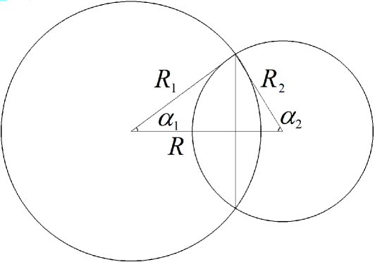
Figure 1: Scheme of eclipsing binary system with spherical components

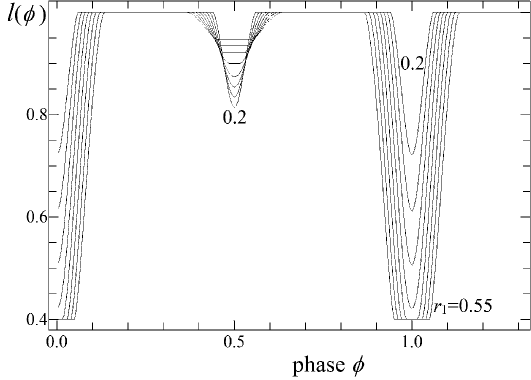
Figure 2: A set of theoretical light curves for the ”simplified” model generated for $R_{1}$ in a range from 0.2 to 0.55 with a step of 0.05 for fixed values of other parameters listed in the text

The square of the eclipsed segment is $S=S_{1}+S_{2}$

$$S_{1}=R_{1}^{2}(\alpha_{1}-\sin\alpha_{1}\cos\alpha_{1}),$$ (1)

$$S_{1}=R_{2}^{2}(\alpha_{2}-\sin\alpha_{2}\cos\alpha_{2}),$$ (2)

where the angles $a_{1},$ $a_{2}$ may be determined from the cosine theorem:

$$\cos\alpha_{1}=\frac{R^{2}+R_{1}^{2}-R_{2}^{2}}{2R_{1}R}=\frac{R^{2}+\eta}{2R_{1}R},$$ (3)

$$\cos\alpha_{2}=\frac{R^{2}+R_{2}^{2}-R_{1}^{2}}{2R_{1}R}=\frac{R^{2}-\eta}{2R_{2}R},$$ (4)

where obviously $\eta=R_{1}^{2}-R_{2}^{2}$ and $|R_{1}-R_{2}|\leq R\leq|R_{1}+R_{2}|$. The total flux is $L=L_{1}+L_{2}$, if $R\geq R_{1}+R_{2}$ (i. e. both stars are visible, $S=0$). For $R\leq R_{1}+R_{2}$, $S=\pi R_{2}^{2}$ (assuming that $R_{2}\leq R_{1}$). Generally, $L=L_{1}+L_{2}\^{a}S/\pi R_{j}^{2}$, where $j$ is the number of star which is behind another, i. e. $j=1,$ if $\cos 2\pi\phi\leq 0,$ and $j=2$, if $\cos 2\pi\phi\geq 0.$ Here $\phi$ is phase ($\phi=0$) corresponds to a full eclipse, independently on which star has larger brightness). For scaling purposes, a dimensionless variable $l(\phi)=L(\phi)/(L_{1}+L_{2})$ is usually introduced. For tests, we used a light curve generated for the following parameters: $R_{1}=0.3,$ $R_{2}=0.2,$ $L_{1}=0.4,$ $L_{2}=0.6$ and $i=80^{\circ}.$ The phases were computed with a step of 0.02. This light curve as well as other generated for a set of values of $R_{1}$ is shown in Fig.2. As a test function we have used:

$$F=\sum_{i=1}^{n}\frac{(x_{i}-\alpha x_{c}(\phi_{i}))^{2}}{\sigma_{i}^{2}},$$ (5)

where $x_{i}$(or $l_{i}$) are values of the signal at phases $\phi_{i}$ with a corresponding accuracy estimate $\sigma_{i},$ and $x_{c}$ are theoretical values computed for a given trial set of $m$ parameters. For normally distributed errors and absence of systematic differences between the observations and theoretical values, the parameter $F$ is a random variable with $X_{n-m}^{2}$ a statistical distribution (Ander:2003; Cher:1993). For the analysis carried out in this work, we used a simplified model with $\sigma_{i}=1$. This assumption does not challenge the basic properties of the test function. The scaling parameter is sometimes determined as $x(0.75)/x_{c}(0.75)$, i. e. at a phase where both components are visible, and the flux (intensity) has its theoretical maximum (in the âno spotsâ model). To improve statistical accuracy, it may be recommended to use a scaling parameter computed for all real observations:

$$\alpha=\frac{\sum_{i=1}^{n}\frac{x_{i}}{\sigma_{i}^{2}}}{\sum_{i=1}^{n}\frac{x_{c}(\phi_{i})}{\sigma_{i}^{2}}},$$ (6)

This corresponds to a least squares estimate of a scaling parameter. I. e the model value of the out–of–eclipse intensity $L=L_{1}+L_{2}$ may be theoretically an any positive number, and these parameters may be ”independent”. By introducing $l_{1}=L_{1}/L$ and $l_{2}=L_{2}/L,$ we get an obvious relation $l_{2}=1-l_{1},$ i. e. one parameter. For $L,$ sometimes are used values at the observed light curve at the phase 0.75 (i. e when both stars are to be visible so maximal light). We prefer instead to use all the data with scaling as in Eq.(6). Even in our simplified model, the number of parameters is still large (4). At Fig.4, the lines of equal levels of $F$ are shown. One may see that the zones of small values are elongated and inclined showing a high correlation between estimates of 2 parameters. In fact this correlation is present for other pairs of parameters. This means that there may be relatively large regions in the multiâparameter space which produce theoretical light curves of nearly equal coincidence with observations.

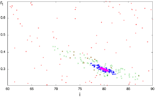
Figure 3: Best 100 points after $10^{2},$ $10^{3},$ $10^{4},$ $10^{5}$ trial computations, respectively.

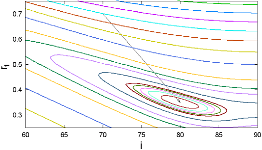
Figure 4: Lines of equal values of the test function $F$ for fixed values of other parameters. The arrow shows position of the âtrueâ parameters used to generate the signal.

In the software by (Zol:2010), the Monte-Carlo method is used, and at each trial computation of the light curve, the random parameters are used in a corresponding range: $C_{k}=C_{k,min}+(C_{k,min}-C_{k,min}){\rm rand},$ where rand is an uniformly distributed random value. Then one may plot âparameter â parameterâ diagrams for âbestâ points after a number of $N$ trial computations. The âbestâ means sorting of sets of the parameters according to the values of the test function $F$. Initially, the points are distributed uniformly. With an increasing $N$, âbetterâ (with smaller $F$) point concentrate to a minimum. There may be some local minima, if the number of parameters will be larger (e.g. spot(s) present in the atmosphere(s) of component(s)). We had made computations for an artificial function of $m(=1,2,3)$ variables (And:2013a). The minimal value $\delta$ (as a true value was set to zero), which was obtained using $N$ trial computations in the Monte-Carlo method is statistically proportional to

$$\delta\propto N^{-2/m},$$ (7)

i.e. the number of computations $N\propto\delta^{-m/2}$ drastically increases with both an increasing accuracy and number of parameters. For our simplified model, the numerical experiments statistically support this relation. Also, the distance between the âsuccessful computationsâ (when the test function becomes smaller than all previous ones) $\Delta N\propto N$. Obviously, it is not realistic to make computations of the test function for billions times to get a set of statistically optimal parameters. In the âbrute forceâ method, the test functions are computed using a grid in the $m$ â dimensional space, so the interval of each parameter is divided by $n_{i}$ points. The number of computations is $N=n_{1}n_{2}\^{a}\'{S}...n_{m}$ should be still large. Either the Monte Carlo method, or the âbrute forceâ one allow to determine positions of the possible local extrema in an addition to the global one. However, if the preliminary position is determined, one should use faster methods to reach the minimum. Classically, there may be used the method of the âsteepest descentâ (also called the ”gradient descent”), where the new set of parameters may be determined as

$$C_{k+1,i}=C_{k,i}-\lambda h_{k,i},$$ (8)

where $C_{k,i}$ is the estimated value of the coefficient $C_{i}$ at $k$-th iteration, $h_{k,i}$ â proposed vector of direction for the coefficient $C_{i}$, and $\lambda$ is a parameter. Typically one may use one of the methods for one–dimensional minimization (Pres:2007; Kor:1968), determine a next set of the parameters $C_{k,i}$, recompute a new vector $h_{k,i}$ and again minimize $\lambda.$ In the method of the steepest descent, one may use a $h_{k,i}=\partial F/\partial C_{i}$ gradient as a simplest approximation to this vector. Another approach (Newton-Raphson) is to redefine a function $F(\lambda)=F(C_{i},i=1...m)$, compute the root of equation $\partial F/\partial\lambda=0,$ and then to use a parabolic approximation to this function. Thus

$$\lambda=(\partial F/\partial\lambda)/(\partial^{2}F/\partial\lambda^{2}).$$ (9)

There may be some modifications of the method based on a decrease of $\lambda$, which may be recommended, if the shape of the function significantly differs from a parabola. In the method of âconjugated gradientsâ, the function is approximated by a second-order polynomial. Finally it is usually recommended to use the (Marq:1963) algorithm. We tested this algorithm with a combination of the âsteepest descentâ (when the determinant of the Hessian matrix is negative) and âconjugated gradientsâ