Order-invariant prior specification in Bayesian factor analysis

Abstract.

In (exploratory) factor analysis, the loading matrix is identified only up to orthogonal rotation. For identifiability, one thus often takes the loading matrix to be lower triangular with positive diagonal entries. In Bayesian inference, a standard practice is then to specify a prior under which the loadings are independent, the off-diagonal loadings are normally distributed, and the diagonal loadings follow a truncated normal distribution. This prior specification, however, depends in an important way on how the variables and associated rows of the loading matrix are ordered. We show how a minor modification of the approach allows one to compute with the identifiable lower triangular loading matrix but maintain invariance properties under reordering of the variables.

1. Introduction

Let $y$ be an $m$-vector of observed random variables, which for simplicity we take to be centered. Let $f\sim N_{k}(0,I_{k})$ be a standard normal $k$-vector of latent factors, with $k\leq m$. The factor analysis model postulates that

(1.1) $${y}={\beta}{f}+{\varepsilon},$$

where $\beta=(\beta_{ij})\in\mathbb{R}^{m\times k}$ is an unknown loading matrix, and $\varepsilon\sim N_{m}(0,\Omega)$ is an $m$-vector of normally distributed error terms that are independent of $f$. The error terms are assumed to be mutually independent with $\Omega=\text{diag}(\omega^{2}_{1},\dots,\omega^{2}_{m})$ comprising $m$ unknown positive variances that are also known as uniquenesses. This model with an unrestricted $m\times k$ loading matrix $\beta$ is sometimes referred to as exploratory factor analysis—in contrast to confirmatory factor analysis, which refers to situations in which some collection of entries of $\beta$ is modeled as zero.

Integrating out the latent factors $f$ in (1.1), the observed random vector $y$ is seen to follow a centered multivariate normal distribution with covariance matrix

(1.2) $$\Sigma=\Omega+\beta\beta^{\prime}.$$

As discussed in detail in Anderson and Rubin (1956), $\Sigma$ determines the unrestricted loading matrix $\beta$ only up to orthogonal rotation. Indeed, $\beta\beta^{\prime}=\beta QQ^{\prime}\beta^{\prime}$ for any $k\times k$ orthogonal matrix $Q$. More details on factor analysis can be found, for instance, in Bartholomew et al. (2011), Drton et al. (2007), and Mulaik (2010).

In this paper, we are concerned with Bayesian inference in (exploratory) factor analysis. In Bayesian computation, it is convenient to impose an identifiability constraint on the loading matrix $\beta$. A common choice is to restrict $\beta$ to be lower triangular with nonnegative diagonal entries, that is, $\beta_{ij}=0$ for $1\leq i<j\leq k$ and $\beta_{ii}\geq 0$ for $1\leq i\leq k$ (Geweke and Zhou, 1996, Aguilar and West, 2000, Lopes and West, 2004). Under these constraints, a full rank matrix $\beta$ is uniquely determined by $\beta\beta^{\prime}$. In the papers just referenced and also the software implementation provided by Martin et al. (2011), a default prior on the lower triangular loading matrix has all its non-zero entries independent with

(1.3) $$\beta_{ij} \sim\begin{cases}\mathit{TN}(0,C_{0})&\text{ if }i=j,\\ N(0,C_{0})&\text{ if }i>j.\end{cases}$$

Here, $\mathit{TN}(0,C_{0})$ denotes a truncated normal distribution on $(0,\infty)$, i.e., the conditional distribution of $X$ given $X>0$ for $X\sim N(0,C_{0})$. The variance $C_{0}>0$ is a hyperparameter. The prior distribution for the uniquenesses has $\omega_{1}^{2},\dots,\omega_{m}^{2}$ independent of $\beta$ and also mutually independent with Inverse Gamma distribution,

(1.4) $$\omega_{i}^{2} \sim\mathit{IG}(\nu/2,\nu s^{2}/2)$$

for hyperparameters $\nu,s>0$. Equivalently, $\nu s^{2}/\omega_{i}^{2}$ is chi-square distributed with $\nu$ degrees of freedom; compare Eqn. (26) in Geweke and Zhou (1996).

As discussed in Lopes and West (2004, Sect. 6), the prior specification in (1.3) is such that the induced prior on $\beta\beta^{\prime}$ and the covariance matrix $\Sigma$ in (1.2) depends on the way the variables and the associated rows of the loading matrix $\beta$ are ordered. Indeed, a priori,

(1.5) $$(\beta\beta^{\prime})_{ii}/C_{0}=\sum_{j=1}^{k}\beta_{ij}^{2}/C_{0}=\sum_{j=1}^{\min\{i,k\}}\beta_{ij}^{2}/C_{0}$$

follows a chi-square distribution with degrees of freedom $\min\{i,k\}$. Consequently, the implied prior and also the posterior distribution for the covariance matrix $\Sigma$ is not invariant under permutations of the variables.

In this paper we propose a modification of the prior distribution for $\beta$ that maintains the convenience of computing with an identifiable lower triangular loading matrix all the while making the prior distributions of $\beta\beta^{\prime}$ and $\Sigma$ invariant under reordering of the variables. Our proposal, described in Section 2, merely changes the prior distributions of the diagonal entries $\beta_{ii}$ in (1.3), which will be taken from a slightly more general family than the truncated normal. The details of a Gibbs sampler to draw from the resulting posterior are given in Section 3. We conclude with numerical examples and a discussion in Sections 4 and 5, respectively.

2. Order-invariant prior distribution

Without any identifiability constraints, the loading matrix $\beta$ takes its values in all of $\mathbb{R}^{m\times k}$. A natural default prior would then be to take all entries $\beta_{ij}$, $i=1,\dots,m$ and $j=1,\dots,k$, to be independent $N(0,C_{0})$ random variables; we write $\beta\sim N_{m\times k}(0,C_{0}I_{m}\otimes I_{k})$. The spherical normal distribution $N_{m\times k}(0,C_{0}I_{m}\otimes I_{k})$ is clearly invariant under permutation of the rows of the matrix. Hence, the induced prior distribution of $\beta\beta^{\prime}$ and of the covariance matrix $\Sigma$ from (1.2) is invariant under simultaneous permutation of rows and columns.

Working with the prior just described comes at the cost of losing the identifiability of $\beta$. However, this can be overcome as follows. Assuming that $m\geq k$, any $m\times k$ matrix $\beta$ with linearly independent columns can be uniquely decomposed as $\beta=LQ$, where $L$ is an $m\times k$ lower triangular matrix with positive diagonal, and $Q$ is a $k\times k$ orthogonal matrix. We may then use the implied distribution of the lower triangular matrix $L$ as a prior on the loading matrix. The following theorem about the joint distribution of $L$ and $Q$ is adapted from Theorem $2.1.13$ in Muirhead (1982).

Theorem 2.1.

Let $\beta=LQ$ be the LQ decomposition of the $m\times k$ random matrix $\beta\sim N_{m\times k}(0,C_{0}I_{m}\otimes I_{k})$, where $m\geq k$. Then the lower triangular matrix $L$ and the orthogonal matrix $Q$ are independent, the distribution of $Q$ is the normalized Haar measure, and the distribution of $L=(L_{ij})$ has joint density proportional to

(2.1) $$\prod_{i=1}^{m}\prod_{j=1}^{\min\{i,k\}}\exp\left\{-\frac{1}{2C_{0}}L_{ij}^{2}\right\}\times\prod_{i=1}^{k}L_{ii}^{k-i}\mathbf{1}_{\{L_{ii}>0\}}$$

with respect to the Lebesgue measure on the space of $m\times k$ lower triangular matrices.

The joint distribution for the entries of $L=(L_{ij})$ given by (2.1) has the entries $L_{ij}$, $i\geq j$, independent with $L_{ij}\sim N(0,C_{0})$ if $i>j$ and $L_{ii}$ following the distribution with density proportional to

(2.2) $$x^{k-i}\exp\left\{-\frac{1}{2C_{0}}x^{2}\right\},\quad x>0.$$

Note that $L_{kk}\sim\mathit{TN}(0,C_{0})$. The joint distribution for a lower triangular matrix in (2.1) thus differs from that given by (1.3) only in the coordinates $L_{ii}$ for $1\leq i\leq k-1$, which are no longer truncated normal.

Assume as in (1.4) that $\Omega$ and $\beta$ are independent a priori. Then since $Q$ is independent of $L$, and

$$\Sigma=\Omega+\beta\beta^{\prime}=\Omega+LQQ^{\prime}L^{\prime}=\Omega+LL^{\prime}$$

does not depend on $Q$, the tuple $(y,\Omega,L,\Sigma)$ is independent of $Q$. Hence, $(\Omega,L,\Sigma)$ is also independent of $Q$ a posteriori (i.e., conditional on $y$). Our proposal is now simply to keep with the standard identifiability constraint that has the loading matrix $\beta$ lower triangular with nonnegative diagonal entries but to use the distribution given by (2.1) instead of (1.3) for this lower triangular loading matrix. Concerning the remaining parts of the prior specification, we continue to assume independence of $\beta$ and $\Omega$, and we stick with the choice from (1.4) for the prior on the uniquenesses. This proposed prior has then the property that the distributions of $\beta\beta^{\prime}$ and the covariance matrix $\Sigma$ are invariant under reordering of the variables (i.e., matrix rows and columns), both a priori and a posteriori.

3. Gibbs sampler

Consider now an actual inferential setting in which we observe a sample $y_{1},\dots,y_{n}$ that comprises $n$ independent random vectors drawn from a distribution in the $k$-factor model. Let $Y$ be the $n\times m$ matrix with the vectors $y_{1},\dots,y_{n}$ as rows. Let $F$ be an associated $n\times k$ matrix whose rows $f_{1},\dots,f_{n}$ are independent vectors of latent factors. The factor analysis model dictates that

(3.1) $${Y}={F}{\beta}^{\prime}+E,$$

where $E=(\varepsilon_{1},\dots,\varepsilon_{n})^{\prime}$ is an $n\times m$ matrix of stochastic errors. The pairs $(f_{t},\varepsilon_{t})$ for $1\leq t\leq n$ are independent, and in each pair $f_{t}\sim N_{k}(0,I_{k})$ and $\varepsilon_{t}\sim N_{m}(0,\Omega)$ are independent as well. The unknown parameters are comprised in the matrices $\Omega=\text{diag}(\omega^{2}_{1},\dots,\omega^{2}_{m})$ and $\beta=(\beta_{ij})\in\mathbb{R}^{m\times k}$, where the latter is restricted to be lower triangular with nonnegative diagonal.

We now adopt the prior distribution on $\beta$ and $\Omega$ given by (2.1) and (1.4), and derive the full conditionals needed for a Gibbs sampler that generates draws from the posterior distribution of $(\beta,\Omega)$. As in Lopes and West (2004), we write

$$\beta_{i}=\begin{cases}(\beta_{i1},\dots,\beta_{ii})^{\prime}&\text{ if }i\leq k,\\ (\beta_{i1},\dots,\beta_{ik})^{\prime}&\text{ if }i>k,\end{cases}$$

and explicitly involve the latent factors in $F$. Let $F_{i}$ be the $n\times i$ matrix made up of the first $i$ columns of $F$, and write $Y_{i}$ for the $i$-th column of $Y$ (in contrast to $y_{t}$, which is the $t$-th row of $Y$). The full conditionals for $F$, $\Omega$ and $\beta$ are determined as follows. First, the rows $f_{t}$ of $F$ are conditionally independent given $(\beta,\Omega,Y)$ with

(3.2) $$(f_{t}\,|\,\beta,\Omega,Y)\;\sim\;N_{k}\left((I_{k}+\beta^{\prime}\Omega^{-1}\beta)^{-1}\beta^{\prime}\Omega^{-1}y_{t},({I}_{k}+{\beta}^{\prime}{\Omega}^{-1}{\beta})^{-1}\right)$$

for $t=1,\dots,n$. Second, the uniquenesses $\omega_{1}^{2},\dots,\omega_{m}^{2}$ are conditionally independent given $(\beta,F,Y)$ with

(3.3) $$(\omega^{2}_{i}\,|\,\beta,F,Y)\;\sim\;\mathit{IG}\left(\tfrac{1}{2}(\nu+T),\tfrac{1}{2}(\nu s^{2}+d_{i})\right),$$

where

$$d_{i}=({Y}_{i}-{F}_{i}{\beta}_{i}^{\prime})^{\prime}({Y}_{i}-{F}_{i}{\beta}_{i}^{\prime}).$$

Third, the rows of $\beta$ are conditionally independent given $(\Omega,F,Y)$. For $i=1,\dots,k$, the conditional density of the vector $\beta_{i}$ is proportional to

(3.4) $$\beta_{ii}^{k-i}\frac{1}{\det(C_{i})}\exp\left\{-\frac{1}{2}({\beta}_{i}-{m}_{i})^{\prime}{C}_{i}^{-1}({\beta}_{i}-{m}_{i})\right\}\mathbf{1}_{\{\beta_{ii}>0\}},$$

where

$${C}_{i}=\left(\frac{1}{C_{0}}{I}_{i}+\frac{1}{\omega_{i}^{2}}{F}_{i}^{\prime}{F}_{i}\right)^{-1}\quad\text{and}\quad{m}_{i}=\frac{1}{\omega_{i}^{2}}{C}_{i}{F}_{i}^{\prime}{Y}_{i}.$$

For $i=k+1,\dots,m$, the conditional distribution is

(3.5) $$({\beta}_{i}\,|\,\Omega,F,Y)\;\;\sim\;N_{k}({m}_{i},{C}_{i})$$

with

$${C}_{i}=\left(\frac{1}{C_{0}}{I}_{k}+\frac{1}{\omega_{i}^{2}}{F}^{\prime}{F}\right)^{-1}\quad\text{and}\quad{m}_{i}=\frac{1}{\omega_{i}^{2}}{C}_{i}{F}^{\prime}{Y}_{i}.$$

The only full conditional that differs from those given in Lopes and West (2004) is the one for $\beta_{i}$ with $i\leq k$ from (3.4). To draw from this distribution, we first sample from $(\beta_{ii}\,|\,\Omega,F,Y)$ and then from $(\beta_{i1},\dots,\beta_{ii-1}\,|\,\beta_{ii},\Omega,F,Y)$. The latter distribution is a multivariate normal distribution. The only new challenge is thus the sampling from $(\beta_{ii}\,|\,\Omega,F,Y)$, which has density proportional to

$$\beta_{ii}^{k-i}e^{-\frac{(\beta_{ii}-a)^{2}}{2b^{2}}}{\bf 1}_{\{\beta_{ii}>0\}}$$

for constants $a\in\mathbb{R}$ and $b>0$ determined by $(\Omega,F,Y)$. After scaling $\beta_{ii}$ by $b$, the problem reduces to generating draws from distributions with density in the class

(3.6) $$f(x\,|\,\alpha,\gamma)=\frac{1}{Z(\alpha,\gamma)}x^{\alpha-1}e^{-(x-\gamma)^{2}},\quad x>0,$$

where $\alpha>0$ and $\gamma\in\mathbb{R}$ are two parameters, and $Z(\alpha,\gamma)$ is the normalizing constant. In the present context, integer values of $\alpha$ are of interest. The densities in (3.6) are log-concave, and we use adaptive rejection sampling (Gilks and Wild, 1992) as implemented in the R package ars to generate from them.

4. Numerical experiments

We illustrate the use of the two different priors, obtained from (1.3) and (2.1), respectively, on a simulated dataset $Y$ that involves $m=15$ variables and is of size $n=30$. The data are drawn from the $k=3$ factor distribution given by the following loading matrix and uniquenesses:

$$\beta_{0}=\bordermatrix{&\scriptstyle 1&\scriptstyle 2&\scriptstyle 3\cr\scriptstyle 1&0.97&0&0\cr\scriptstyle 2&0.04&0.90&0\cr\scriptstyle 3&1.00&-1.12&0.57\cr\scriptstyle 4&2.03&0.42&0.57\cr\scriptstyle 5&0.31&0.47&0.09\cr\scriptstyle 6&0.43&-0.21&-0.35\cr\scriptstyle 7&0.75&0.31&0.68\cr\scriptstyle 8&0.45&-0.48&-1.50\cr\scriptstyle 9&-2.21&1.45&0.38\cr\scriptstyle 10&1.98&-0.30&0.96\cr\scriptstyle 11&-2.63&0.41&1.09\cr\scriptstyle 12&-0.72&1.39&0.97\cr\scriptstyle 13&-0.88&2.01&-0.39\cr\scriptstyle 14&-0.53&0.04&0.59\cr\scriptstyle 15&-0.95&1.39&0.37\cr},\qquad\text{diag}(\Omega_{0})=\bordermatrix{&\cr\scriptstyle 1&0.17\cr\scriptstyle 2&0.05\cr\scriptstyle 3&0.02\cr\scriptstyle 4&0.02\cr\scriptstyle 5&0.05\cr\scriptstyle 6&0.06\cr\scriptstyle 7&0.04\cr\scriptstyle 8&0.67\cr\scriptstyle 9&-0.04\cr\scriptstyle 10&0.21\cr\scriptstyle 11&0.10\cr\scriptstyle 12&0.09\cr\scriptstyle 13&0.21\cr\scriptstyle 14&0.51\cr\scriptstyle 15&0.03\cr}.$$

We create a second data matrix $Y^{\pi}$ by permuting the columns of $Y$ based on the permutation $\pi$ from Table 1, i.e. the $i$-th column of $Y$ becomes the $\pi(i)$-th column of $Y^{\pi}$. For Bayesian inference, we choose the hyperparameters as Lopes and West (2004), that is, $C_{0}=1$, $\nu=2.2$ and $s=\sqrt{0.1/2.2}$. Via Gibbs sampling, we draw from the posterior distributions for the covariance matrix $\Sigma=\Omega+\beta\beta^{\prime}$ for each data set, focusing on the factor analysis models $k=3$, and $k=6$ factors. The Gibbs samplers are initialized at the respective maximum likelihood estimates for $(\beta,\Omega)$. After a burnin of $10,000$ iterations, we ran each sampler for $300,000$ iterations.

Table 1. The permutation $\pi$ used to reorder simulated data.

$i$	1	2	3	4	5	6	7	8	9	10	11	12	13	14	15
$\pi(i)$	10	14	13	15	12	6	7	2	11	9	8	3	5	1	4

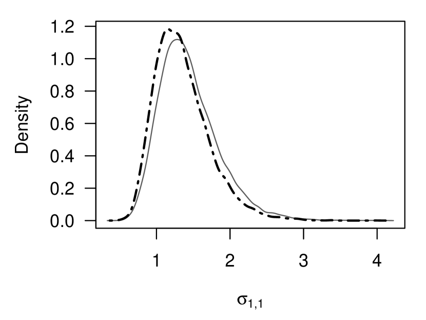
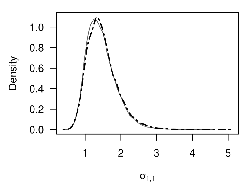
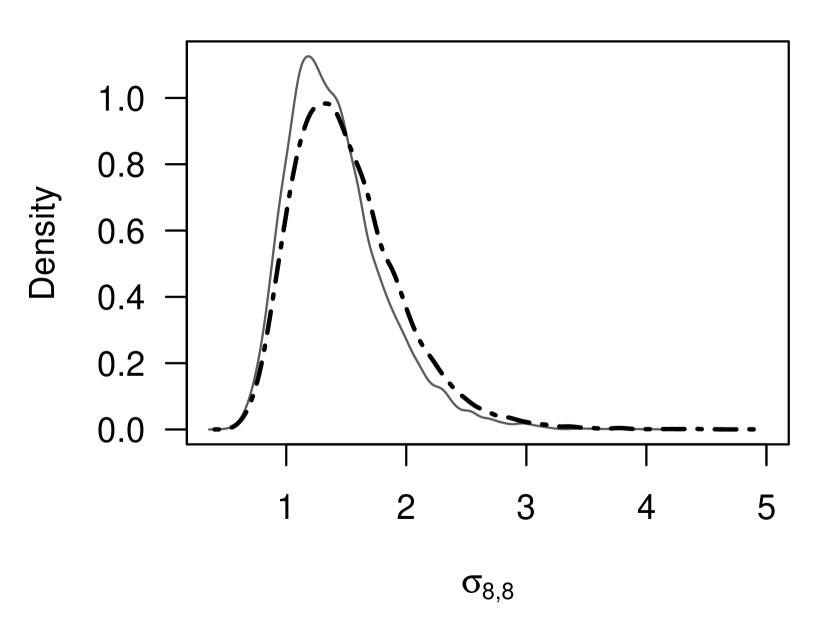
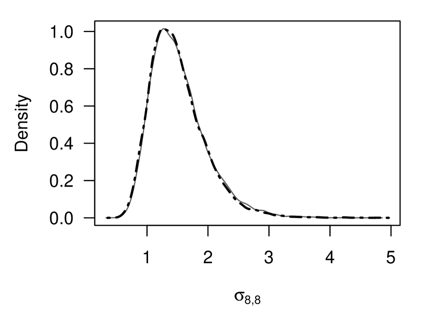
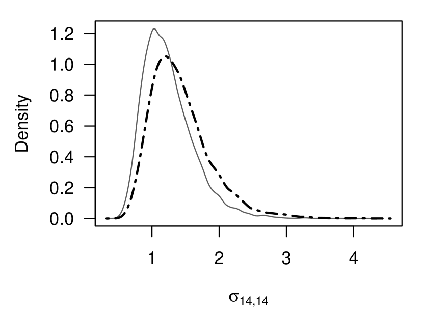
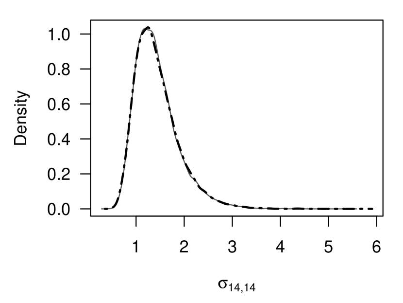
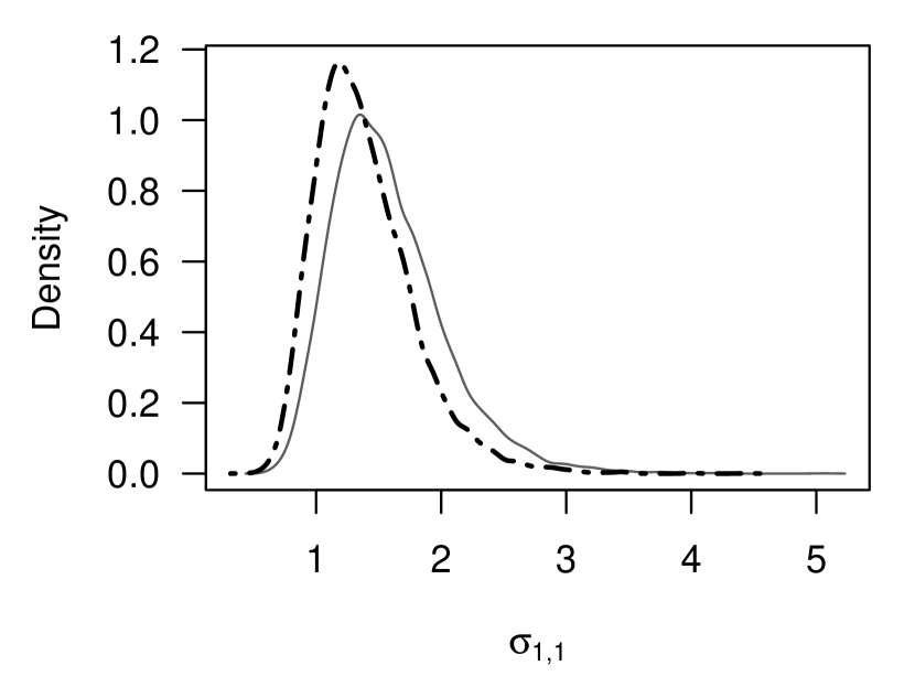
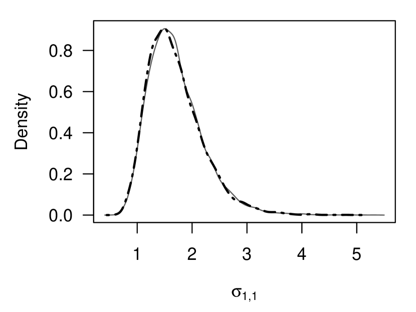
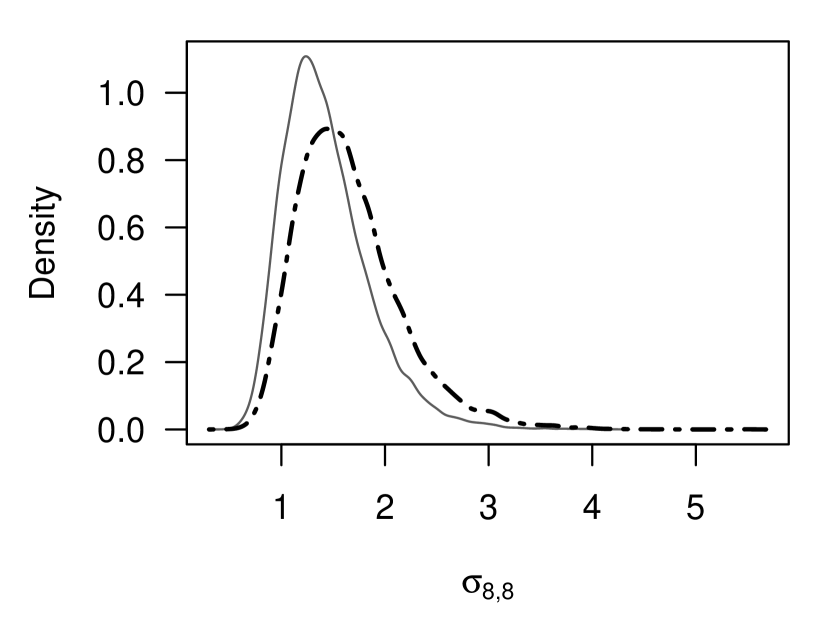
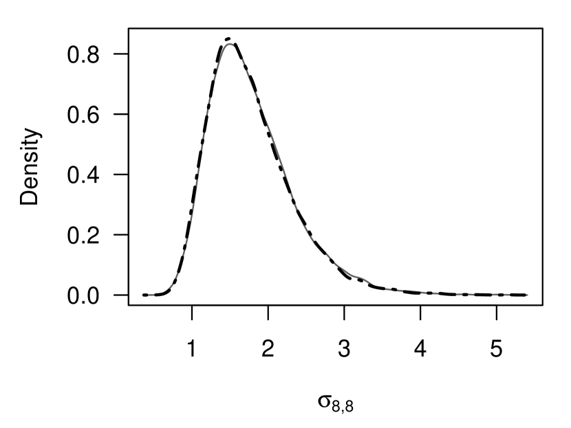
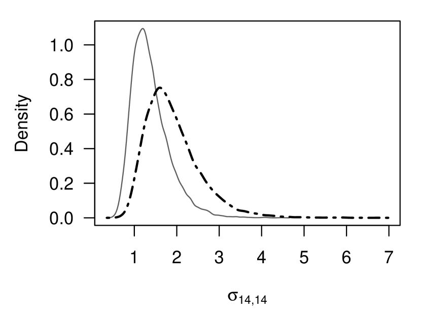
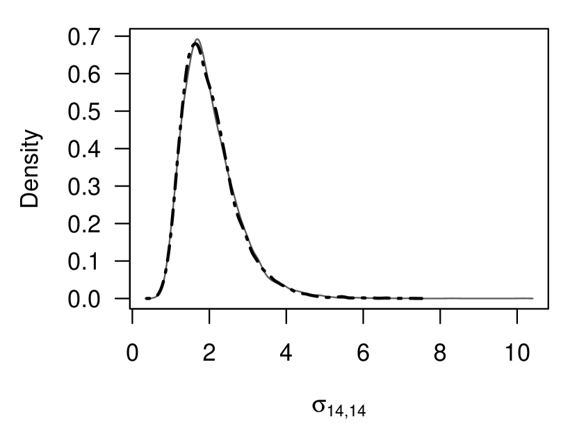
Figures 4.1 and 4.2 show kernel density estimates of the posterior densities of selected variances. More precisely, we compare the densities of $(\sigma_{ii}\,|\,Y)$ and $(\sigma_{\pi(i),\pi(i)}\,|\,Y^{\pi})$ for $i=1,8,14$. Under our proposed prior from (2.1), the two posterior densities are the same. Indeed, the plots in the right hand columns of Figures 4.1 and 4.2 show only minor discrepancies due to Monte Carlo error. The ‘standard prior’ from (1.3), however, results in visible differences that are more pronounced for $k=6$, which is not surprising as larger differences are possible among the degrees of freedom of the chi-square prior for $(\beta\beta^{\prime})_{ii}/C_{0}$; recall (1.5). Note that the observed shifts in the posterior distributions under the ‘standard prior’ are explained by the different chi-square degrees of freedom.

Figure 4.1. Posterior densities of $(\sigma_{ii}\,|\,Y)$, in black, and of $(\sigma_{\pi(i),\pi(i)}\,|\,Y^{\pi})$, in grey, in factor analysis with $k=3$ factors, for $i=1,8,14$. The left column concerns the prior from (1.3), and the right column is based on the prior proposed in (2.1).

Figure 4.2. Posterior densities of $(\sigma_{ii}\,|\,Y)$, in black, and of $(\sigma_{\pi(i),\pi(i)}\,|\,Y^{\pi})$, in grey, in factor analysis with $k=6$ factors, for $i=1,8,14$. The left column concerns the prior from (1.3), and the right column is based on the prior proposed in (2.1).

5. Conclusion

This paper proposes a prior distribution for the loading matrix in factor analysis. The proposal allows for computation with an identifiable lower triangular loading matrix $\beta$ all the while having the associated covariance matrix invariant under permutation of the variables at hand. The prior is intended as a possible default when there is no reason to impose dependence among loadings or to treat the loadings of different variables differently. Concerning possible departures from our default scenario, we remark that the software of Martin et al. (2011) also allows one to impose patterns of zeros in the loading matrix $\beta$. As mentioned earlier, the latter situation is sometimes termed confirmatory factor analysis. The identifiability issues we addressed need not arise in that case as orthogonal transformations will generally not preserve prescribed zeros in the loading matrix.

Sampling from the posterior distribution resulting from the prior we proposed is largely the same as for the ‘standard prior’ that has been used by several authors including Geweke and Zhou (1996) and Lopes and West (2004). The key difference is the need to sample from distributions in the class specified by (3.6). These distributions also appear in the realm of multivariate $t$-distributions (Finegold and Drton, 2011, 2014), although a square-root transformation is necessary to match the setup there. It thus seems worthwhile to develop an efficient sampler targeting precisely this family of distributions, which is a problem we are working on.

Finally, we emphasize that our proposal rests in an important way on the fact that we derived it from a spherical joint normal distribution for the loading matrix, namely, $\beta\sim N_{m\times k}(0,C_{0}I_{m}\otimes I_{k})$. Departures from this situation, even merely including a non-zero mean for this matrix normal distribution, seem to lead to a considerably more difficult scenario.

References

- Aguilar and West (2000) Aguilar, O. and West, M. (2000). “Bayesian dynamic factor models and variance matrix discounting for portfolio allocation.” Journal of Business & Economic Statistics, 18(3): 338–357.
- Anderson and Rubin (1956) Anderson, T. W. and Rubin, H. (1956). “Statistical inference in factor analysis.” In Proceedings of the Third Berkeley Symposium on Mathematical Statistics and Probability, 1954–1955, vol. V, 111–150. University of California Press, Berkeley and Los Angeles.
- Bartholomew et al. (2011) Bartholomew, D., Knott, M., and Moustaki, I. (2011). Latent variable models and factor analysis. Wiley Series in Probability and Statistics. John Wiley & Sons, Ltd., Chichester, third edition. A unified approach.
- Drton et al. (2007) Drton, M., Sturmfels, B., and Sullivant, S. (2007). “Algebraic factor analysis: tetrads, pentads and beyond.” Probab. Theory Related Fields, 138(3-4): 463–493.
- Finegold and Drton (2011) Finegold, M. and Drton, M. (2011). “Robust graphical modeling with classical and alternative -distributions.” Annals of Applied Statistics, 5(2A): 1057–1080.
- Finegold and Drton (2014) — (2014). “Robust Bayesian graphical modeling using Dirichlet -distributions.” Bayesian Analysis, 9(3): 521–550.
- Geweke and Zhou (1996) Geweke, J. and Zhou, G. (1996). “Measuring the pricing error of the arbitrage pricing theory.” The Review of Financial Studies, 9(2): 557–587.
- Gilks and Wild (1992) Gilks, W. R. and Wild, P. (1992). “Adaptive rejection sampling for Gibbs sampling.” Applied Statistics, 41(2): 337–348.
- Lopes and West (2004) Lopes, H. F. and West, M. (2004). “Bayesian model assessment in factor analysis.” Statist. Sinica, 14(1): 41–67.
- Martin et al. (2011) Martin, A. D., Quinn, K. M., and Park, J. H. (2011). “MCMCpack: Markov Chain Monte Carlo in R.” Journal of Statistical Software, 42(9): 22.
- Muirhead (1982) Muirhead, R. J. (1982). Aspects of multivariate statistical theory. John Wiley & Sons, Inc., New York. Wiley Series in Probability and Mathematical Statistics.
- Mulaik (2010) Mulaik, S. A. (2010). Foundations of factor analysis. Statistics in the Social and Behavioral Sciences Series. CRC Press, Boca Raton, FL, second edition.