Mean curvature flow with obstacles: a viscosity approach

Abstract

We introduce a level-set formulation for the mean curvature flow with obstacles and show existence and uniqueness of a viscosity solution. These results generalize a well known viscosity approach for the mean curvature flow without obstacle by Evans and Spruck and Chen, Giga and Goto in 1991. In addition, we show that this evolution is consistent with the variational scheme introduced by Almeida, Chambolle and Novaga (2012) and we study the long time behavior of our viscosity solutions.

Keywords:

Mean Curvature Flow, viscosity solutions, long time behavior

Classification:

53C44

1 Introduction

In this article, we introduce the level set formulation for a generalized motion by mean curvature with obstacles. More precisely, let $M(t)=\partial E(t)$ be a family of $n-1$ submanifold in $\mathbb{R}^{n}$, we say that it evolves by mean curvature if for any $x\in M(t)$, the velocity of $M(t)$ at $x$ is given by

$$v(x)=-H\nu(x)$$ (1)

where $H$ is the mean curvature of $M(t)$ at $x$ (nonnegative if $E(t)$ is a convex set with boundary) and $\nu$ is the normal vector to $M(t)$ pointing towards $E(t)^{c}$.

Motivated by recent works from Almeida, Chambolle and Novaga [1] and Spadaro [21] about a discrete scheme for the mean curvature flow with obstacles, we want to constrain (1) forcing

$$\Omega^{-}(t)\subset E(t)\subset\Omega^{+}(t)$$ (2)

where $\Omega^{\pm}$ are two open sets (which can depend on the time variable).

Mean curvature flow has been widely studied in the 30 past years for physical and biological purposes. For instance, one can mention [2, 3] for a new model in biology (tissue repair) using this evolution. Concerning the mathematical study, one can in particular cite [8] for a first paper on this motion, [12] for a geometric study of (1) and [14] and [10] for a level-set formulation and the use of viscosity solutions. In the sequel we follow the last approach.

It is well known (see for example [14]) that if $u:\mathbb{R}^{n}\to\mathbb{R}$ is a smooth function with a nonzero gradient at $x_{0}$, the mean curvature of the level set $\{u=u(x_{0})\}$ at $x_{0}$ is given by $\operatorname{div}\left(\frac{Du}{|Du|}\right)(x_{0}).$ As a result, making this set (and every other level-set of $u$) evolve by mean curvature leads to the following equation for $u$:

$$u_{t}=|Du|\operatorname{div}\left(\frac{Du}{|Du|}\right).$$ (3)

In the whole paper, we will think of $M(t)$ as the zero-level-set of $u(\cdot,t)$.
To add the constraint to (3), we define $u^{\pm}(x,t)$ such that

$$\Omega^{-}(t)\subset E(t)\subset\Omega^{+}(t)\Leftrightarrow\{u^{+}<0\}\subset\{u<0\}\subset\{u^{-}<0\}$$

and impose

$$\forall x,t,\quad u^{-}(x,t)\leqslant u(x,t)\leqslant u^{+}(x,t).$$ (4)

As in [14], [10], we study (3) with constraint (4) using viscosity solutions. We first present a suitable viscosity framework and prove a uniqueness and existence result for bounded uniformly continuous initial data and obstacles and Lipschitz forcing term in the spirit of [11]. Then, we link the regularity of the solution to the regularity of the initial data.

We also show that our level-set approach really defines a geometric flow: the $\alpha$-level set of the solution depends only on the $\alpha$-level set of the initial data and the obstacles. Nonetheless, as expected, there is no real geometrical uniqueness: level sets of the solution can develop non empty interiors because of the obstacles (even if the free evolution does not). In an upcoming paper with Matteo Novaga [20], we study the MCF with obstacles with a geometrical point of view (in the spirit of [12]), proving short time existence, uniqueness and regularity of solutions.

Finally, in Section 4, we compare the approach followed by [21] and [1] (discrete minimizing scheme based on [4]) to ours. More precisely, we show that the discrete scheme has a limit which is the viscosity solution to (3) with constraint (4). In addition, this variational approach gives monotonicity of the flow and therefore information on the long time behavior of the viscosity solution.

2 Notation

In what follows, we consider the equation (slightly more general than (3), but the latter has to be kept in mind), for $u:\mathbb{R}^{n}\times\mathbb{R}^{+}\to\mathbb{R}$

$$\forall t\geqslant 0,x\in\mathbb{R}^{n},\quad u_{t}+F(Du,D^{2}u)+k|Du|=0,$$ (5)

where $k:\mathbb{R}^{n}\times\mathbb{R}^{+}\to\mathbb{R}$ is a forcing term and $F:\mathbb{R}^{n}\times\mathcal{S}_{n}\to\mathbb{R}$ ($\mathcal{S}_{n}$ is the set of symmetric matrices of dimension $n$) satisfies

1. $F\in\mathcal{C}\left(\mathbb{R}^{n}\setminus\{0\}\times\mathcal{S}_{n}(\mathbb{R})\right)$ ,

2. $F$ is geometric : $\forall\lambda>0,\sigma\in\mathbb{R},\;F(\lambda p,\lambda X+\sigma p\otimes p)=\lambda F(p,X)$,

3. For $X$ and $Y$ symmetric matrices with $X\leqslant Y$, $F(p,X)\leqslant F(p,Y)$.

In the following, $Du$ and $D^{2}u$ denote space derivatives only.
We will denote by $u\wedge v$ and $u\vee v$ the quantities $\min(u;v)$ and $\max(u;v)$.

We also introduce $F^{\ast}$ and $F_{\ast}$ which are respectively the upper semicontinuous and lower semicontinuous envelopes of $u$ (see Definition 1).
To play the role of the obstacles, we consider $u^{-}$ and $u^{+}:\mathbb{R}^{n}\times[0,+\infty)\to\mathbb{R}$, with $u^{-}\leqslant u^{+}$. The function $u$ will be forced to stay between $u^{-}$ and $u^{+}$. Geometrically, the constraint reads

$$\{u^{+}<s\}~\subset\{u<s\}\subset\{u^{-}<s\},$$

where, given two functions $u,v:\mathbb{R}^{n}\times[0,\infty)\mapsto\mathbb{R}$, we will denote by

$$\{u=v\}:=\{(x,t)\in\mathbb{R}^{n}\times[0,\infty)\ |\ u(x,t)=v(x,t)\}\quad\text{ and}$$

$$\{u<v\}:=\{(x,t)\in\mathbb{R}^{n}\times[0,\infty)\ |\ u(x,t)<v(x,t)\}.$$

To adapt the classical theory of viscosity solutions (we will use the same scheme of proof as in [11]), the key point is to define correctly sub and super solutions of

$$u_{t}+F(Du,D^{2}u)+k|Du|=0\quad\text{with}\quad u^{-}\leqslant u\leqslant u^{+}.$$ (6)

This definition for two obstacles has been already given, for instance in [23]. To state it, we fisrt need the following notation.

Definition 1.

For $f:\mathbb{R}^{n}\to\mathbb{R}$, we denote by $f^{\ast}$ the upper semicontinuous envelope of $f$. More precisely

$$f^{\ast}(x)=\limsup_{y\to x}f(y).$$

We define in a similar way the lower semicontinuous envelope of $f$.

$$f_{\ast}(x)=\liminf_{y\to x}f(y).$$

Note that $f^{\ast}$ (resp. $f_{\ast}$) is the smallest (resp. largest) semicontinuous function $g$ such that $g\geqslant f$ (resp. $g\leqslant f$).

We are now ready to give the main definition.

Definition 2.

A function $u:\mathbb{R}^{n}\times\mathbb{R}^{+}\to\mathbb{R}$ is said to be a (viscosity) subsolution on $[0,T)$ of the motion equation with obstacles $u^{+},u^{-}$ and initial condition $u_{0}$ if

• $u$ is upper semicontinous (usc),

• for all $(x,t)\in\mathbb{R}^{n}\times[0,T),\,u^{-}(x,t)\leqslant u(x,t)\leqslant u^{+}(x,t)$,

• for all $x\in\mathbb{R}^{n}$, $u(x,0)\leqslant u_{0}(x)$,

• if $\varphi$ is a $\mathcal{C}^{2}$ function of $x,t$, if $(\hat{x},\hat{t})\in\mathbb{R}^{n}\times(0,T)$ is a maximizer of $u-\varphi$ and if $u(\hat{x},\hat{t})>u^{-}(\hat{x},\hat{t})$, then, at $(\hat{x},\hat{t})$,

  $$\varphi_{t}+F_{\ast}(D\varphi,D^{2}\varphi)+k|D\varphi|\leqslant 0.$$

Similarly, $u$ is said to be a (viscosity) supersolution of the motion equation with obstacles $u^{+},u^{-}$ and initial condition $u_{0}$ if

• $u$ is lower semicontinous (lsc),

• for all $(x,t)\in\mathbb{R}^{n}\times[0,T),\,u^{-}(x,t)\leqslant u(x,t)\leqslant u^{+}(x,t)$,

• for all $x\in\mathbb{R}^{n}$, $u(x,0)\geqslant u_{0}(x)$,

• if $\varphi$ is a $\mathcal{C}^{2}$ function of $x,t$, if $(\hat{x},\hat{t})\in\mathbb{R}^{n}\times(0,T)$ is a minimizer of $u-\varphi$ and if $u(\hat{x},\hat{t})<u^{+}(\hat{x},\hat{t})$, then at $(\hat{x},\hat{t})$,

  $$\varphi_{t}+F^{\ast}(D\varphi,D^{2}\varphi)+k|D\varphi|\geqslant 0.$$

Finally, $u$ is said to be a (viscosity) solution of the motion equation with obstacles $u^{+},u^{-}$ if $u$ is both a super and a sub solution.
To simplify, we write

$$u_{t}+F(Du,D^{2}u)+k|Du|=0\quad\text{on }\{u^{-}\leqslant u\leqslant u^{+}\}.$$ (7)

A supersolution (resp subsolution) of the motion equation with obstacles $u^{+},u^{-}$ will be called a supersolution (resp. subsolution) of (7).

Looking at the very definition, one can make the

Remark 1.

Let $u$ be a subsolution with obstacles $u^{-}\leqslant u^{+}$. Then, $u$ is a subsolution with obstacles $u^{-}$ and $v^{+}$ for every $v^{+}\geqslant u^{+}.$
The obstacle $u^{-}$ is a subsolution whereas $u^{+}$ is a supersolution.

Remark 2.

It has to be noticed that using this definition, obstacles can depend on the time variable. Moreover, the contact zone $\{u^{+}=u^{-}\}$ can be nonempty.

We also want to point out that the obstacle problem can be defined using a modified $F$ (see [11], Example 1.7). For instance, let

$$G(x,t,u,u_{t},Du,D^{2}u)=\max\left(\min\left(u_{t}+F(Du,D^{2}u),u-u^{-}\right),u-u^{+}\right).$$ (8)

One can easily show that the (usual) viscosity solutions of $G=0$ coincide with our definition above (the only difference is the subsolutions of $G=0$ do not have to satisfy $u\geqslant u^{-}$, but must remain below $u^{+}$). Nonetheless (8) cannot be written of the form

$$u_{t}+\tilde{G}(x,t,u,Du,D^{2}u)=0,$$

which is the usual form for parabolic equations, for which known results (see [11, 16, 10]) could apply. Thus, despite of this convenient formulation, we have to check that the usual results still apply. That is why we decided to use the definition above with a standard function $F$ but with (explicit) obstacles.

There is another equivalent definition of such solutions, which can be useful (see [11]).

Definition 3.

Let $f:\mathbb{R}^{n}\times(0,T)\to\mathbb{R}$. We said that $(a,p,X)\in\mathbb{R}\times\mathbb{R}^{n}\times\mathcal{S}_{n}(\mathbb{R})$ is a superjet for $f$ at $(x_{0},t_{0})$ and we denote $(a,p,X)\in\mathcal{P}^{2,+}f(x_{0},t_{0})$ if, for $(x,t)\to(x_{0},t_{0})$ in $\mathbb{R}^{n}\times(0,T)$,

$$f(x,t)\leqslant f(x_{0},t_{0})+a(t-t_{0})+\left\langle p\,,\,x-x_{0}\right\rangle+\frac{1}{2}\left\langle X(x-x_{0})\,,\,x-x_{0}\right\rangle+o(|t-t_{0}|+|x-x_{0}|^{2}).$$

We likewise say that $(a,p,X)\in\mathbb{R}\times\mathbb{R}^{n}\times\mathcal{S}_{n}(\mathbb{R})$ is a subjet for $f$ at $(x_{0},t_{0})$ and we denote $(a,p,X)\in\mathcal{P}^{2,-}f(x_{0},t_{0})$ if, for $(x,t)\to(x_{0},t_{0}),$

$$f(x,t)\geqslant f(x_{0},t_{0})+a(t-t_{0})+\left\langle p\,,\,x-x_{0}\right\rangle+\frac{1}{2}\left\langle X(x-x_{0})\,,\,x-x_{0}\right\rangle+o(|t-t_{0}|+|x-x_{0}|^{2}).$$

Then, $u$ is a subsolution of (7) if it satisfies the three first assumptions of the previous definition and if

$$\forall(x,t)\in\mathbb{R}^{n}\times(0,T),\ (a,p,X)\in\mathcal{P}^{2,+}u(x,t),\quad u(x,t)>u^{-}(x,t)\Rightarrow a+F_{\ast}(p,X)+k|p|\leqslant 0.$$

Of course, $u$ is a supersolution of (7) if the three assumptions of the first definition are satisfied and if

$$\forall(x,t)\in\mathbb{R}^{n}\times(0,T),\ (a,p,X)\in\mathcal{P}^{2,-}u(x,t),\quad u(x,t)<u^{+}(x,t)\Rightarrow a+F^{\ast}(p,X)+k|p|\geqslant 0.$$

3 Existence and uniqueness

The aim of this section is to show the

Theorem 1.

We assume that $u^{-}$ and $u^{+}$ are uniformly continuous and bounded and that $k$ is Lipschitz. Then, if $u_{0}:\mathbb{R}^{n}\to\mathbb{R}$ is uniformly continuous and $u^{-}(x,0)\leqslant u_{0}(x)\leqslant u^{+}(x,0)$, (7) has an unique solution, which is uniformly continuous.

The structure of the proof is classical when dealing with viscosity solutions. A comparison principle will show uniqueness, and existence will follow by standard methods.
In what follows, $L$ is a Lipschitz constant of $k$ and $\omega$ is a modulus of continuity for $u_{0}$, $u^{-}$ and $u^{+}$.

3.1 Uniqueness

We begin by proving a comparison principle, adapted from [11], Theorem 8.2. It has to be noticed that the same result with no obstacles has been proved in [16] (Th. 4.1) in a very general framework. We could adapt this result to the obstacle case but we prefer to present a simpler and self consistent proof based on [11] (nonetheless, we will use some ideas of [16]).

Proposition 1 (Comparison principle).

We assume that $u$ is a subsolution and $v$ a supersolution of $\eqref{vsol}$ on $(0,T)$, and that $u(x,0)\leqslant v(x,0)$. Then, $u\leqslant v$ in $\mathbb{R}^{n}\times(0,T)$.

Proof.

We proceed by contradiction. Since for every $c$ sufficiently small, we can find $\eta>0$ such that $\tilde{u}=(u-\frac{\eta}{T-t})\vee u^{-}$ is still a subsolution, but with

$$F(D\tilde{u},D^{2}\tilde{u})+k|D\tilde{u}|\leqslant-c<0,$$

it is enough to prove the comparison principle with $\tilde{u}$ and then pass to the limit (nonetheless, we still write $u$). Suppose that there exists $\overline{x},\overline{t}$ such that $u(\overline{x},\overline{t})-v(\overline{x},\overline{t})\geqslant 2\delta>0.$ One defines

$$\Phi(x,y,t)=u(x,t)-v(y,t)-\frac{\alpha}{4}|x-y|^{4}-\frac{\varepsilon}{2}(|x|^{2}+|y|^{2}).$$

If $\varepsilon$ is sufficiently small, $\Phi(\overline{x},\overline{x},\overline{t})\geqslant\delta.$ Hence, $M:=\max\limits_{x,y,t}\Phi(x,y,t)\geqslant\delta$ (the penalization at infinity $\frac{1}{2}\varepsilon(|x|^{2}+|y|^{2})$ reduces searching for the maximum to a compact set). Let $\hat{x},\hat{y},\hat{t}$ be a maximum point. Since $u$ and $v$ are bounded, there is $C$ depending only on $\|u\|_{\infty}$ and $\|v\|_{\infty}$ such that

$$|\hat{x}-\hat{y}|\leqslant\frac{C}{\alpha^{1/4}}.$$

First, let us show by contradiction that $u(\hat{x},\hat{t})>u^{-}(\hat{x},\hat{t})$ and $v(\hat{y},\hat{t})<u^{+}(\hat{y},\hat{t})$. Suppose for example that $u(\hat{x},\hat{t})=u^{-}(\hat{x},\hat{t})$. Then

$$0<\delta \leqslant u^{-}(\hat{x},\hat{t})-v(\hat{y},\hat{t})\leqslant u^{-}(\hat{y},\hat{t})+\omega(|\hat{x}-\hat{y}|)-v(\hat{y},\hat{t})$$

$$\leqslant\omega(|\hat{x}-\hat{y}|)+0\leqslant\omega(C\alpha^{-1/4}).$$

Hence, if $\alpha$ is sufficiently large (independently of $\varepsilon$), $\omega(C\alpha^{-1/4})\leqslant\delta/3$. Contradiction (this shows moreover that $\hat{t}<T$). Similarly, $v(\hat{y},\hat{t})<u^{+}(\hat{y},\hat{t})$.

In what follows, $\alpha$ is fixed sufficiently big to satisfy these conclusions.

As

$$M+\alpha|x-y|^{4}+\frac{\varepsilon}{2}(|x|^{2}+|y|^{2})\geqslant u(x,t)-v(y,t)$$ (9)

with equality in $\hat{x},\hat{y},\hat{t}$, we are able to apply Ishii’s lemma [11] to

$$u(x,t)-v(y,t)-\Phi(x,y,t)\quad\text{ where }\quad\Phi(x,y,t)=M+\alpha|x-y|^{4}+\frac{\varepsilon}{2}(|x|^{2}+|y|^{2})$$

which provides, for every $\mu>0$, $(a,b,X,Y)$ such that $(a,\underbrace{\alpha|\hat{x}-\hat{y}|^{2}(\hat{x}-\hat{y})}_{=:\hat{p}}-\varepsilon\hat{y},Y)\in\overline{\mathcal{P}}^{2,+}v(\hat{y},\hat{t})$ and $(b,\alpha|\hat{x}-\hat{y}|^{2}(\hat{x}-\hat{y})+\varepsilon\hat{x},X)\in\overline{\mathcal{P}}^{2,-}u(\hat{x},\hat{t})$. It provides moreover $a-b=0$ and

$$-\left(\frac{1}{\mu}+\|A\|\right)\begin{bmatrix}I&0\\ 0&I\end{bmatrix}\leqslant\begin{bmatrix}X&0\\ 0&-Y\end{bmatrix}\leqslant A+\mu A^{2},$$

where

$$A=D^{2}\Phi(\hat{x},\hat{y},\hat{t})=\begin{bmatrix}P&-P\\ -P&P\end{bmatrix}+\varepsilon\begin{bmatrix}I&0\\ 0&I\end{bmatrix}$$

and

$$P=2\alpha(\hat{x}-\hat{y})\otimes(\hat{x}-\hat{y})+\alpha|\hat{x}-\hat{y}|^{2}.$$

That shows in particular that $X-Y\leqslant\varepsilon^{2}I$ and $\|X\|,\|Y\|\leqslant C_{1}\left(\alpha|\hat{x}-\hat{y}|^{2}+\varepsilon\right).$

Since $u$ and $v$ are respectively subsolution and supersolution near $(\hat{x},\hat{t})$ and $(\hat{y},\hat{t})$, one has

$$c\leqslant a-b+F^{\ast}(\hat{p}-\varepsilon\hat{y},Y-\varepsilon I)-F_{\ast}(\hat{p}+\varepsilon\hat{x},X+\varepsilon I)+k(\hat{y},\hat{t})|\hat{p}-\varepsilon y|-k(\hat{x},\hat{t})|\hat{p}+\varepsilon\hat{x}|.$$

One can write

$$k(\hat{y},\hat{t})|\hat{p}+\varepsilon\hat{y}|-k(\hat{x},\hat{t})|\hat{p}-\varepsilon x|\\ \leqslant(k(\hat{y},\hat{t})-k(\hat{x},\hat{t}))|\hat{p}+\varepsilon\hat{y}|+2|k(\hat{x},\hat{t})|(|\varepsilon\hat{y}|+|\varepsilon\hat{x}|),$$

which gives, with $a-b=0$,

$$c\leqslant F^{\ast}(\hat{p}-\varepsilon y,Y-\varepsilon I)-F_{\ast}(\hat{p}+\varepsilon\hat{x},X+\varepsilon I)\\ +L(|\hat{x}-\hat{y}|)|\hat{p}+\varepsilon\hat{y}|+2\|k\|_{\infty}(|\varepsilon\hat{x}|+|\varepsilon\hat{y}|).$$

Then, we want to let $\varepsilon$ go to 0.
Since $M\geqslant\delta>0$, we have

$$\delta+\frac{1}{4}\alpha|\hat{x}-\hat{y}|^{4}+\frac{\varepsilon}{2}(|\hat{x}|^{2}+|\hat{y}|^{2})\leqslant u(\hat{x},\hat{t})-v(\hat{y},\hat{t})\leqslant\|u\|_{\infty}+\|v\|_{\infty},$$

which implies that $\varepsilon|\hat{x}|^{2}$ is bounded, hence $\varepsilon\hat{x}\to 0$ (same for $\varepsilon\hat{y}$), whereas for $i\in\{2,3,4\},$ $\alpha|\hat{x}-\hat{y}|^{i}$ is bounded (so is $\hat{p}$, $X$ and $Y$). Indeed, $\alpha$ is fixed here. Hence one can assume that $\hat{p}\to p$, $X\to X_{0}$, $\alpha|\hat{x}-\hat{y}|^{4}\to\mu_{\alpha}.$
We now use a short lemma, which is an easy adaptation of [16], Proposition 4.4 (see also Lemma 2.8 in the preprint of [15], which has a form which is closer to ours) and whose proof is reproduced here for convenience.

Lemma 1.

One has

$$\lim_{\alpha\to\infty}\lim_{\varepsilon\to 0}\alpha|\hat{x}-\hat{y}|^{4}=0.$$

Proof.

Let

$$M_{h}=\sup\limits_{\begin{subarray}{c}|x-y|\leqslant h\\ t\in[0,T)\end{subarray}}(u(x,t)-v(y,t))$$

and $(x_{h}^{n},y_{h}^{n},t_{h}^{n})$ such that $u(x_{h}^{n},t_{h}^{n})-v(y_{h}^{n},t_{h}^{n})\geqslant M_{h}-\frac{1}{n}$ and $|x_{h}^{n}-y_{h}^{n}|\leqslant h.$ Then,

$$M_{h}-\frac{1}{n}-\frac{\alpha h^{4}}{4}-\frac{\varepsilon}{2}\left(|x_{h}^{n}|^{2}+|y_{h}^{n}|^{2}\right)\leqslant M\leqslant u(\hat{x},\hat{t})-v(\hat{y},\hat{t}).$$

As $x_{h}^{n}$ and $y_{h}^{n}$ do not depend on $\varepsilon$, one can let it go to zero (considering the liminf of the right term) to get

$$M_{h}-\frac{1}{n}-\frac{\alpha h^{4}}{4}\leqslant\liminf_{\varepsilon\to 0}(u(\hat{x},\hat{t})-v(\hat{y},\hat{t})).$$

Let $h\to 0$ (We denote by $M^{\prime}$ the decreasing limit of $M_{h}$). One obtains

$$M^{\prime}-\frac{1}{n}\leqslant\liminf_{\varepsilon\to 0}(u(\hat{x},\hat{t})-v(\hat{y},\hat{t})).$$

Let $\alpha$ go to infinity:

$$M^{\prime}-\frac{1}{n} \leqslant\liminf_{\alpha\to\infty}\liminf_{\varepsilon\to 0}(u(\hat{x},\hat{t})-v(\hat{y},\hat{t}))$$

$$\leqslant\limsup_{\alpha\to\infty}\left(\sup_{\begin{subarray}{c}|x-y|\leqslant C\alpha^{-1/4}\\ t\in[0,T)\end{subarray}}(u(x,t)-v(y,t))\right)$$

$$\leqslant\limsup_{h\to 0}\sup_{|x-y|\leqslant h}(u(x,t)-v(y,t))=M^{\prime}$$

hence

$$\lim_{\alpha\to\infty}\lim_{\varepsilon\to 0}u(\hat{x},\hat{t})-v(\hat{y},\hat{t})=M^{\prime}.$$

We prove similarly that $\lim\limits_{\alpha\to\infty}\lim\limits_{\varepsilon\to 0}M=M^{\prime}$. As a matter of fact,

$$\lim_{\alpha\to\infty}\lim_{\varepsilon\to 0}\left(\alpha|\hat{x}-\hat{y}|^{4}+\frac{\varepsilon}{2}(|\hat{x}|^{2}+|\hat{y}|^{2})\right)=0,$$

which proves the lemma. ∎

One can now choose $\alpha$ such that $\lim\limits_{\varepsilon\to 0}\alpha|\hat{x}-\hat{y}|^{4}\to\mu_{\alpha}$ with $\mu_{\alpha}\leqslant c/2L$ and pass to the liminf in $\varepsilon\to 0$. One gets (using $X\leqslant Y+\varepsilon^{2}I$),

$$\frac{c}{2}\leqslant\liminf\left(F_{\ast}(\hat{p},X)-F^{\ast}(\hat{p},X)\right).$$

To conclude, we distinguish two cases:

• if $p\neq 0$, then $F^{\ast}(p,X_{0})=F_{\ast}(p,X_{0})$ and we get the contradiction.

• if $p=0$, we have $\alpha|\hat{x}-\hat{y}|^{2}(\hat{x}-\hat{y})\underset{\varepsilon\to 0}{\longrightarrow}0$, so $X_{0}=0$ and $F^{\ast}(p,X_{0})=F_{\ast}(p,X_{0})=0$ and we get the contradiction too.

∎

3.2 Existence

We will build a solution using Perron’s method. Since we know that the supersolutions of (7) remain larger than subsolutions, the solution, if it exists, must be the largest subsolution (or equivalently, the smallest supersolution). Hence we introduce

$$W(x,t)=\sup\{w(x,t),\;\text{$w$ subsolution on $[0,T)$}\}.$$

We show that $W$ is in fact the expected solution to (7).

Let us first state a straightforward but useful proposition.

Proposition 2.

1. Let $u$ be a subsolution of the motion without obstacles which satisfies $u\leqslant u^{+}$. Then, $u_{ob}:=u\vee u^{-}$ is a subsolution of (7) with obstacles (the same happens for $v\geqslant u^{-}$ supersolution and $v_{ob}=v\wedge u^{+}$).

2. More generally, if $u$ is a solution of the motion with initial conditions $u_{0}$ and obstacles $(u^{-},u^{+})$ and if $v^{-}$ and $v^{+}$ are other obstacles which satisfy $u^{-}\leqslant v^{-}\leqslant u^{+}\leqslant v^{+}$, then $u\vee v^{-}$ is a subsolution of the equation with initial condition $u_{0}\vee v^{-}|_{t=0}$ and obstacles $v^{-}$ and $u^{+}$. In addition, $u$ is a subsolution of the equation with initial conditions $u_{0}$ and obstacles $u^{-}$, $v^{+}$.

Proof.

The proof is quite simple: consider a smooth function $\varphi$ and some $x_{0},t_{0}$ such that $\varphi-u\vee u^{-}$ has a maximum at $(x_{0},t_{0})$. Then, using the definition of subsolutions, either $u(x_{0},t_{0})\vee u^{-}(x_{0},t_{0})=u^{-}(x_{0},t_{0})$ and nothing has to be done, or $u(x_{0},t_{0})>u^{-}(x_{0},t_{0})$. In the second alternative $(x_{0},t_{0})$ is in fact a maximum of $u-\varphi$. Since $u$ is a viscosity subsolution of the motion, we have $\varphi_{t}+F_{\ast}(D\varphi,D^{2}\varphi)+k|D\varphi|\leqslant 0$, what was expected.

Let us now show the second part of the proposition. The initial condition $u\vee v^{-}\leqslant u_{0}\vee v^{-}|_{t=0}$ is satisfied. Once again, we consider $\varphi$ smooth and $(x_{0},t_{0})$ such that $u\vee v^{-}-\varphi$ has a maximum at $(x_{0},t_{0})$. Then, either $u(x_{0},t_{0})\vee v^{-}(x_{0},t_{0})=v^{-}(x_{0},t_{0})$ and nothing has to be checked, or $u(x_{0},t_{0})>v^{-}(x_{0},t_{0})$. The latter implies that $u(x_{0},t_{0})>u^{-}(x_{0},t_{0})$, so $\varphi_{t}+F_{\ast}(D\varphi,D^{2}\varphi)+k|D\varphi|\leqslant 0$, what was wanted. ∎

Lemma 2.

Let $\mathcal{F}$ be a family of subsolutions of (7) and define $U(x,t):=\sup\{u(x,t)),u\in\mathcal{F}\}$. Then, $U^{\ast}$ is a subsolution of (7).

To prove this lemma, we need the following proposition which will be useful later.

Proposition 3.

Let $v$ be a upper semicontinuous function, $(x,t)\in\mathbb{R}^{n}\times\mathbb{R}$ and $(a,p,X)\in\mathcal{P}^{2,+}v(x,t)$. Assume there exists a sequence $(v_{n})$ of usc functions which satisfy

1. There exists $(x_{n},t_{n})$ such that $(x_{n},t_{n},v_{n}(x_{n},t_{n}))\to(x,t,v(x,t))$

2. $(z_{n},s_{n})\to(z,s)$ in $\mathbb{R}^{n}\times\mathbb{R}$ implies $\limsup v_{n}(z_{n},s_{n})\leqslant v(z,s).$

Then, there exists $(\hat{x}_{n},\hat{t}_{n})\in\mathbb{R}^{n}\times\mathbb{R},\;(a_{n},p_{n},X_{n})\in\mathcal{P}^{2,+}v_{n}(\hat{x}_{n},\hat{t}_{n})$ such that

$$(\hat{x}_{n},\hat{t}_{n},v_{n}(\hat{x}_{n},\hat{t}_{n}),a_{n},p_{n},X_{n})\to(x,t,v(x,t),a,p,X).$$

The proof of the proposition and the lemma can be found in [11], Lemma 4.2 and Proposition 4.3 (with obvious changes due to the parabolic situation and obstacles).

In our way to prove that $W$ is the solution of (7), we need to show that it is a subsolution of (7). Lemma 2 shows that $W^{\ast}$ is a subsolution of (7) with obstacles, but without taking the initial condition into account. Indeed even if for all subsolution, one has $u(x,0)\leqslant u_{0}(x)$, which implies $W(x,0)\leqslant u_{0}(x)$, taking the semicontinuous envelope could break this inequality. We thus need to build some continuous barriers which will force $W^{\ast}$ to remain below $u_{0}$ at time zero. More precisely, we build a continuous supersolution $w^{+}$ which gets the initial data $u_{0}$. Then, by comparison principle, every subsolution $u$ will satisfy $u\leqslant w^{+}$ and $W~\leqslant w^{+}$. Taking the envelope will yield

$$W^{\ast}\leqslant(w^{+})^{\ast}=w^{+}$$

which will imply

$$W^{\ast}(x,0)\leqslant u_{0}(x).$$

Similarly, we build a continuous subsolution $w^{-}$ which also gets the initial data. By the very definition of $W$, it gives $W(x,0)\geqslant u_{0}(x).$

For technical reasons, we begin building the solution in the case where $k=0$.

3.2.1 Construction of barriers in the non forcing case

Let us construct $w^{-}$. Without a forcing term, we note that for all $\xi\in\mathbb{R}^{n}$ and $A,B$ with $B$ sufficiently large relatively to $A$,

$$\tilde{h}(x,t)=-(A|x-\xi|^{2}+Bt)$$

is a subsolution of (7) in a neighborhood of $\xi$ but with neither initial conditions nor obstacles. We define

$$h(x,t)=h(x,t)\vee u^{-}(x,t).$$

Then, $h$ is a subsolution (on the full domain, since as soon $|x-\xi|\geqslant\|u^{-}\|_{\infty}/A$, $h(x,t)=u^{-}(x,t)$) of (7), for $A$ sufficiently large uniformly in $\xi$. We then define

$$\theta_{\xi}(r)=\inf\{u_{0}(y)\,\mid\,A|y-\xi|^{2}+r\leqslant 0\}$$

The function $\theta_{\xi}$ is bounded, non decreasing, continuous and satisfies $\theta_{\xi}(0)=u_{0}(\xi)$ and $\theta_{\xi}(-A|x-\xi|^{2}-Bt)\leqslant u_{0}(x).$ As the equation is geometric, $\theta_{\xi}(-A|x-\xi|^{2}-Bt)\vee u^{-}(x,t)$ is also a subsolution. Let us then define

$$\phi(x,t)=\left(\sup_{\xi}\theta_{\xi}(-A|x-\xi|^{2}-Bt)\vee u^{-}(x,t)\right)^{\ast}.$$

Since $\theta_{\xi}(-A|x-\xi|^{2}-Bt)\leqslant u_{0}(x)$ and $u_{0}$ is continuous, we also have $\phi(x,t)\leqslant u_{0}$. In addition, we can check that

$$\phi(x,t)\geqslant\theta_{x}(-A|x-x|^{2}-Bt)=\theta_{x}(-Bt)\geqslant u_{0}(x)-\omega(\sqrt{\frac{Bt}{A}}).$$ (10)

Hence, $\phi(x,0)=u_{0}(x)$. Thanks to Lemma 2, $\phi$ is a subsolution with $\phi(x,0)\leqslant u_{0}(x).$ We conclude this proof defining

$$w^{-}(x,t)=\left(\phi(x,t)-\omega(t)\right)\vee u^{-}(x,t).$$

It is clear that $w^{-}$ is a subsolution with obstacles. Indeed, by definition, $w^{-}\geqslant u^{-}$. Moreover, $\phi(x,t)-\omega(t)\leqslant u_{0}(x)-\omega(t)\leqslant u^{+}(x,0)-\omega(t)\leqslant u^{+}(x,t).$ Proposition 2 concludes the proof.

The other barrier $w^{+}$ is obtained similarly:

$$w^{+}=\left(\inf_{\xi}\theta^{\xi}(A|x-\xi|^{2}+Bt)\wedge u^{+}(x,t)\right)_{\ast}\wedge u^{+}(x,t)$$

with

$$\theta^{\xi}(r)=\sup\{u_{0}(y)\,\mid\,A|y-\xi|^{2}-r\leqslant 0\}.$$

3.2.2 Perron’s method

We have just seen that, thanks to the barriers, $W^{\ast}$ is a subsolution of (7). We now want to show that $W$ is actually a subsolution and that it is also a supersolution.

First, we show uniform continuity of the function $W$, which shows that $W^{\ast}=W$ and therefore, that

Remark 3.

If $k(x,t)=0$, then $W$ is $\omega$-uniformly continuous in space. In time, $W$ is uniformly continuous with modulus $\tilde{\omega}:r\mapsto\max(\omega(r),\omega(\sqrt{\frac{Br}{A}}))$, where $B$ is the constant introduced when constructing the barriers. Indeed, the proof is contained in the following lemma.

Lemma 3.

Let $u(x,t)$ be a subsolution of (7) with no forcing term (and $u_{0},u^{-},u^{+}$ $\omega$-uniformly continuous in space and time). Then, for $t>0$ and $z\in\mathbb{R}^{n}$,

$$u_{z,\delta}(x,t)=(u(x+z,t+\delta)-\omega(|z|)-\tilde{\omega}(|\delta|))\vee u^{-}(x,t)$$

is also a subsolution.

Proof.

To begin, we notice that $u(x+z,t+\delta)-\omega(|z|)-\tilde{\omega}(|\delta|)\leqslant u^{+}(x,t)$.
Now, let $\varphi$ be a smooth function with $\forall x,t$, $u_{z,\delta}(x,t)\leqslant\varphi(x,t)$ with equality at $(\overline{x},\overline{t})$. Then, either $u_{z,\delta}(\overline{x},\overline{t})=u^{-}(\overline{x},\overline{t})$, and nothing has to be done, or $u_{z,\delta}(\overline{x},\overline{t})>u^{-}(\overline{x},\overline{t})$. In the second alternative, we have

$$u(\overline{x}+z,\overline{t}+\delta)-\omega(|z|)-\tilde{\omega}(\delta)>u^{-}(\overline{x},\overline{t})=u^{-}(\overline{x}+z,\overline{t}+\delta)+(u^{-}(\overline{x},\overline{t})-u^{-}(\overline{x}+z,\overline{t}+\delta))$$

hence

$$u(\overline{x}+z,\overline{t}+\delta)>u^{-}(\overline{x}+z,\overline{t}+\delta)+\underbrace{(u^{-}(\overline{x},\overline{t})-u^{-}(\overline{x}+z,\overline{t}+\delta)+\omega(|z|)+\tilde{\omega}(|\delta|))}_{\geqslant 0}\geqslant u^{-}(\overline{x}+z,\overline{t}+\delta).$$

As $u$ is a subsolution at $(\overline{x}+z,\overline{t}+\delta)$ and $u(x+z,t+\delta)\leqslant\varphi(x,t)+\omega(|z|)+\tilde{\omega}(|\delta|)$ with equality at $(\overline{x}+z,\overline{t}+\delta)$, one can write, with $y=x+z,s=t+\delta$,

$$u(y,s)\leqslant\varphi(y-z,s-\delta)+\omega(|z|)+\tilde{\omega}(|\delta|)=:\phi(y,s),$$

equality at $(\overline{y},\overline{s})$ (with $\overline{y}:=\overline{x}+z$ and $\overline{s}=\overline{t}+\delta$), and deduce that $\phi_{t}+F_{\ast}(D\phi(\overline{y},\overline{s}),D^{2}\phi(\overline{y},\overline{s}))\leqslant 0.$ Since $D\phi(\overline{y},\overline{s})=D\varphi(\overline{x},\overline{t})$ (so are the time and spatial second derivatives), we get

$$\varphi_{t}+F_{\ast}(D\varphi(\overline{x},\overline{t}),D^{2}\varphi(\overline{x},\overline{t}))\leqslant 0,$$

what was expected.

Concerning the initial conditions, we have (we use (10) and the comparison principle Proposition 1 between $u$ and $w^{+}$)

$$u(x+z,0+\delta)-\omega(|z|)-\tilde{\omega}(\delta)\leqslant w^{+}(x+z,\delta)-\omega(|z|)-\tilde{\omega}(|\delta|)\leqslant u_{0}(x+z)-\omega(|z|)\leqslant u_{0}(x).$$

∎

Applying this lemma to $W$ shows $(x,t)\mapsto W(x+z,t+\delta)-\omega(|z|)-\tilde{\omega}(|\delta|)\vee u^{-}(x+z,t)$ is a subsolution. By definition of $W$, one can write

$$W(x,t)\geqslant(W(x+z,t+\delta)-\omega(|z|)-\tilde{\omega}(\delta))\vee u^{-}(x+z,t)\geqslant W(x+z,t+\delta)-\omega(|z|)-\tilde{\omega}(\delta)$$

which shows exactly that $W$ is uniformly continuous.

We now want to show that $W$ is in fact a supersolution of (7). We need the following lemma which is adapted from [11], Lemma 4.4.

Lemma 4.

Let $u$ be a subsolution of (7). If $u_{\ast}$ fails to be a solution of $u_{t}+F^{\ast}(Du,D^{2}u)+k|Du|\geqslant 0$ at some $(\hat{x},\hat{t})$ (there exists $(a,p,X)\in\mathcal{P}^{2,-}u_{\ast}(\hat{x},\hat{t})$ such that $a+F^{\ast}(p,X)+k|p|<0$), then for all sufficiently small $\kappa$, there exists a solution $u_{\kappa}$ of $u_{t}+F_{\ast}(Du,D^{2}u)+k|Du|\leqslant 0$ satisfying $u_{\kappa}(x,t)\geqslant u(x,t)$, $\sup\limits_{\mathbb{R}^{n}}(u_{\kappa}-u)>0$, $u_{\kappa}(x,t)\leqslant u^{+}(x,t)$ and such that $u$ and $u_{\kappa}$ coincide for all $|x-\hat{x}|,|t-\hat{t}|\geqslant\kappa.$

Proof.

We can suppose that $u_{\ast}$ fails to be a supersolution at $(0,1)$ (this implies in particular $u_{\ast}(0,1)<u^{+}(0,1)$). We get $(a,p,X)\in\mathcal{P}^{2,-}u_{\ast}(0,1)$ such that $a+F^{\ast}(p,X)+k(0,1)|p|<0$. We introduce for $\gamma,\delta,r>0$,

$$u_{\delta,\gamma}(x,t)=u_{\ast}(0,1)+\delta+\left\langle p\,,\,x\right\rangle+a(t-1)+\frac{1}{2}\left\langle Xx\,,\,x\right\rangle-\gamma(|x|^{2}+t-1).$$

By upper semicontinuity of $F^{\ast}$, $u_{\delta,\gamma}$ is a subsolution of $u_{t}+F^{\ast}(Du,D^{2}u)+k|Du|\leqslant 0$ on $B_{r}((0,1))$ for $\gamma,\delta,r$ sufficiently small.
Since

$$u(x,t)\geqslant u_{\ast}(x,t)\geqslant u_{\ast}(0,1)+a(t-1)+\left\langle p\,,\,x\right\rangle+\frac{1}{2}\left\langle Xx\,,\,x\right\rangle+o(|x|^{2})+o(|t-1|),$$

choosing $\delta=\gamma\frac{r^{2}+r}{8}$, we get $u(x,t)>u_{\delta,\gamma}(x,t)$ for $\frac{r}{2}\leqslant|x|,|t-1|\leqslant r$ and $r$ sufficiently small. Moreover, we can reduce $r$ again to have $u_{\delta,\gamma}\leqslant u^{+}$ on $B_{r}$ (Choosing $r$ sufficiently small, one has $\delta$ sufficiently small and $u_{\delta,\gamma}(0,1)-u_{\ast}(0,1)=\delta<u^{+}(0,1)-u_{\ast}(0,1)$. By continuity, one can find a smaller $r$ such that $u_{\delta,\gamma}(x,t)<u^{+}(x,t)$ for all $\frac{r}{2}\leqslant|x|,|t-1|\leqslant r$.).
Thanks to Lemma 2, the function

$$\tilde{u}(x,t)=\left\{\begin{matrix}\max(u(x,t),u_{\delta,\gamma}(x,t))\text{ if }|x,t-1|<r\\ u(x,t)\text{ otherwise}\end{matrix}\right.$$

is a subsolution of (7) (with initial conditions if $r$ is small enough). ∎

Now, we saw that $W$ is a subsolution of (7) (in particular, $W\leqslant u^{+}$). If it is not a supersolution at a point $\hat{x},\hat{t}$ , Lemma 4 provides $W_{\kappa}\geqslant W$ subsolutions of (7) (with initial condition, even if we have to reduce $r$ again, to make $t$ stay far from zero), which is a contradiction with the definition of $W$.
Finally, $W$ is the expected solution of (7).

3.2.3 With forcing term

1. We assume at this point only that $u^{-},u^{+}$ and $u_{0}$ are $K$-Lipschitz in space. Then, thanks to Remark 3, there exists a $K$-Lipschitz (in space) solution $\psi$ of the non forcing term equation. Let us set $w^{-}(x,t)=(\psi(x,t)+\|k\|_{\infty}Kt)\vee u^{-}(x,t).$ It satisfies, as soon as $w^{-}>u^{-}$,

   $$u_{t}-\|k\|_{\infty}K+F(Du,D^{2}u)=0,\qquad u(x,0)=u_{0}(x).$$

   As a consequence, $w^{-}$ is a continuous subsolution of (7) (with forcing term) satisfying $w^{-}(x,0)=u_{0}(x)$. It is a barrier as in 3.2.1. We build $w^{+}$ in a similar way and apply Perron’s method to see that $W$ is a solution.

2. Here, $u^{+}$, $u^{-}$ and $u_{0}$ are only $\omega$-uniformly continuous. For all $K>0$, let $u^{0}_{K}=\min\limits_{y}u_{0}(y)+K|x-y|$, $u^{+}_{K}(x,t)=\max\limits_{y}u^{+}(y,t)-K|x-y|$ and $u^{-}_{K}=\min\limits_{y}u_{0}(y)+K|x-y|.$ These three new function are $K$-Lipschitz in space and converge uniformly (in space) to $u_{0},u^{+}$ and $u^{-}$ when $K\to\infty.$ Moreover, as $u_{0},u^{+},u^{-}$ are $\omega$-uniformly continuous, so are they.
   Thanks to the previous point, for every $K$, there exists a solution $u_{K}$ of (7) with obstacles $u^{+}_{K},u^{-}_{K}$ and with initial data $u^{0}_{K}$, which is (thanks to the following proposition 4, which is admitted for a little time) uniformly continuous with same moduli on $[0,T]$ for every $T$. One can define, thanks to Ascoli’s theorem

   $$u(x,t)=\lim_{n}u_{K_{n}}(x,t).$$

   The function $u$ is continuous. We have to check that it is the solution of the motion with obstacles $u^{\pm}$.

   It is clear that $u^{-}\leqslant u\leqslant u^{+}$. Let $\varphi$ be a smooth function and $(\hat{x},\hat{t})$ a maximum point of $u-\varphi$ such that $u(\hat{x},\hat{t})-u^{-}(\hat{x},\hat{t})=:\eta>0$. One can assume that the maximum is strict. We then choose $\varepsilon$ such that

   $$\forall(x,t)\in B_{\varepsilon}(\hat{x},\hat{t}),\quad u(x,t)-u^{-}(x,t)\geqslant\frac{3\eta}{4}.$$

   Let

   $$\delta:=\min_{\partial B_{\varepsilon}}|u-\varphi|.$$

   It is positive (since the maximum is strict, possibly reducing $\varepsilon$). We choose $n_{0}$ such that

   $$\forall n\geqslant n_{0},\;\|u-u_{K_{n}}\|_{L^{\infty}(B_{\varepsilon})},\ \|u^{-}-u^{-}_{K_{n}}\|_{L^{\infty}(B_{\varepsilon})}\leqslant\max\left(\frac{\eta}{4},\,\frac{\delta}{2}\right).$$

   Then, for every $n\geqslant n_{0}$, $u_{K_{n}}-\varphi$ has a maximum $(x_{n},t_{n})$ on $B_{\varepsilon}$ reached out of $u^{-}_{K_{n}}$. It is easy to show that $(x_{n},t_{n})\to(\hat{x},\hat{t})$. Since $u_{K_{n}}$ is a viscosity subsolution, one can write, at $(x_{n},t_{n})$,

   $$\varphi_{t}+F_{\ast}(D\varphi,D^{2}\varphi)+k|D\varphi|\leqslant 0.$$

   By smoothness of $\varphi$ and semicontinuity of $F_{\ast}$, we get the same inequality at $(\hat{x},\hat{t})$.

   We prove that $u$ is a supersolution using the same arguments.

Let us conclude this section by an estimation of the solution’s regularity, which is essentially [15], Lemma 2.15 (except that the solution here is only uniformly continuous).

Proposition 4.

Let $u$ be the unique solution of (7). Then $u$ is uniformly continuous in space. moreover, one as

$$\forall(x,y,t),\quad|u(x,t)-u(y,t)|\leqslant\omega(e^{Lt}|x-y|).$$

Proof.

First, it is well known that one can choose $\omega$ to be continuous and nondecreasing. Since $u$ and $v$ are bounded, $\omega\wedge(\|u\|_{\infty}+\|v\|_{\infty})$ is a modulus too. In the following, we use this new modulus, still denoted by $\omega$.

Then, let $\rho_{n}$ be a $\mathcal{C}^{\infty}$ nondecreasing function on $[0,\infty[$ such that $0\leqslant\rho_{n}-\omega$, for all $r>n+1$, $\rho_{n}(r)=2N+1$, and for all $r\in[0,n],\rho_{n}(r)-\omega(r)\leqslant\frac{1}{n}.$ We define

$$\omega_{n}(r)=\rho_{n}+\frac{r}{n^{2}}.$$

It’s clear that $\omega_{n}(r)\underset{n\to\infty}{\longrightarrow}\omega(r).$ Moreover, for a fixed $n$, $\omega^{\prime}_{n}(r)$ is bounded and remains far from zero. In what follows, we work with $\omega_{n}$.

We will proceed as in Proposition 1. Let $\phi(x,y,t)=\omega_{n}(e^{Lt}|x-y|).$ We will show by contradiction that $u(x,t)-u(y,t)\leqslant\phi(x,y,t).$ Assume that

$$M:=\sup_{(x,y,t)\in\mathbb{R}^{n}\times\mathbb{R}^{n}\times[0,T)}u(x,t)-u(y,t)-\phi(x,y,t)>0.$$

As before, we introduce

$$\tilde{M}=\sup_{x,y,t\leqslant T}u(x,t)-u(y,t)-\phi(x,y,t)-\frac{\alpha}{2}(|x|^{2}+|y|^{2})-\frac{\gamma}{T-t}.$$

For sufficiently small $\gamma,\alpha$, $\tilde{M}$ remains positive and is attained (at $\overline{x},\overline{y},\overline{t}<T)$. As $u_{0}$ is $\omega$-uniformly continuous, $\overline{t}>0.$ Moreover, since $u$ is continuous, $|\overline{x}-\overline{y}|$ is bounded away from zero, independently of $\alpha$ and $\gamma$.

By assumption, $u^{-}(\overline{x},\overline{t})\leqslant u^{-}(\overline{y},\overline{t})+\omega(|\overline{x}-\overline{y}|)\leqslant u^{-}(\overline{y},\overline{t})+\omega_{n}(|\overline{x}-\overline{y}|)\leqslant u(\overline{y},\overline{t})+\phi(\overline{x},\overline{y},\overline{t})$ so $0\leqslant\tilde{M}<u(\hat{x},\hat{t})-u(\hat{y},\hat{t})-\phi(\hat{x},\hat{y},\hat{t})$ forces $u(\overline{x},\overline{t})>u^{-}(\overline{x},\overline{t}).$ Similarly, $u(\overline{y},\overline{t})<u^{+}(\overline{y},\overline{t}).$

Applying Ishii’s lemma ([11], Th. 8.3) to $\tilde{u}(x,t)=u(x,t)-\frac{\alpha}{2}|x|^{2}$ and $\tilde{v}(y,t)=u(y,t)+\frac{\alpha}{2}|y|^{2}$ where

$$\overline{p}=D_{x}\phi=\frac{\overline{x}-\overline{y}}{|\overline{x}-\overline{y}|}e^{L\overline{t}}\omega_{n}^{\prime}(e^{L\overline{t}}|\overline{x}-\overline{y}|)=-D_{y}\phi\neq 0,$$

$$Z=D^{2}_{x}\phi=\frac{e^{L\overline{t}}}{|\overline{x}-\overline{y}|}\omega_{n}^{\prime}(e^{L\overline{t}}|\overline{x}-\overline{y}|)I+\frac{(\overline{x}-\overline{y})\otimes(\overline{x}-\overline{y})}{|\overline{x}-\overline{y}|^{3}}e^{Lt}\omega_{n}^{\prime}(e^{L\overline{t}}|\overline{x}-\overline{y}|)\\ +\frac{(\overline{x}-\overline{y})\otimes(\overline{x}-\overline{y})}{|\overline{x}-\overline{y}|^{2}}e^{2L\overline{t}}\omega_{n}^{\prime\prime}(e^{L\overline{t}}|\overline{x}-\overline{y}|).$$

and

$$A=D^{2}\phi=\begin{bmatrix}Z&-Z\\ -Z&Z\end{bmatrix},$$

we get the following. For all $\beta$ such that $\beta A<I$, there exists $\tau_{1},\tau_{2}\in\mathbb{R}$, $X,Y\in\mathcal{S}_{n}$ such that

$$\tau_{1}-\tau_{2}=\frac{\gamma}{(T-t)^{2}}+Le^{L\overline{t}}|\overline{x}-\overline{y}|\omega_{n}^{\prime}(e^{Lt}|\overline{x}-\overline{y}|),$$

$$(\tau_{1},\overline{p}+\alpha\overline{x},X+\alpha I)\in\overline{\mathcal{P}}^{2,+}u(\overline{x},\overline{t}),$$

$$(\tau_{2},\overline{p}-\alpha\overline{y},Y-\alpha I)\in\overline{\mathcal{P}}^{2,-}u(\overline{y},\overline{t}),$$

$$\frac{-1}{\beta}\begin{bmatrix}I&0\\ 0&I\end{bmatrix}\leqslant\begin{bmatrix}X&0\\ 0&-Y\end{bmatrix}\leqslant(I-\beta A)^{-1}A.$$

In particular, the last equation provides $X\leqslant Y$.

As $u$ is a subsolution and a supersolution, one has

$$\tau_{1}+k(\overline{x},\overline{t})|\overline{p}+\alpha\overline{x}|+F_{\ast}(\overline{p}+\alpha\overline{x},X+\alpha I)\leqslant 0,$$ (11)

$$\tau_{2}-k(\overline{y},\overline{t})|\overline{p}-\alpha\overline{y}|+F^{\ast}(\overline{p}-\alpha\overline{y},Y-\alpha I)\geqslant 0.$$

$X\leqslant Y$ in the last equation gives

$$-\tau_{2}+k(\overline{y},\overline{t})|\overline{p}-\alpha\overline{y}|-F^{\ast}(\overline{p}-\alpha\overline{y},X-\alpha I)\leqslant 0.$$ (12)

Adding (12) to (11) leads to

$$\frac{\gamma}{(T-\overline{t})^{2}}+Le^{L\overline{t}}|\overline{x}-\overline{y}|\omega_{n}^{\prime}(e^{L\overline{t}}|\overline{x}-\overline{y}|)-k(\overline{x},\overline{t})|\overline{p}+\alpha\overline{x}|+k(\overline{y},\overline{t})|\overline{p}-\alpha\overline{y}|\\ +F_{\ast}(\overline{p}+\alpha\overline{x},X+\alpha I)-F^{\ast}(\overline{p}-\alpha\overline{y},X-\alpha I)\leqslant 0.$$ (13)

Notice that

$$Le^{L\overline{t}}|\overline{x}-\overline{y}|\omega_{n}^{\prime}(e^{L\overline{t}}|\overline{x}-\overline{y}|)-k(\overline{x},\overline{t})|\overline{p}|+k(\overline{y},\overline{t})|\overline{p}|\\ \geqslant Le^{L\overline{t}}|\overline{x}-\overline{y}|\omega_{n}^{\prime}(e^{L\overline{t}}|\overline{x}-\overline{y}|)-L|\overline{x}-\overline{y}|e^{L\overline{t}}\omega_{n}^{\prime}(e^{L\overline{t}}|\overline{x}-\overline{y}|)\geqslant 0.$$ (14)

Then, (13) becomes

$$\frac{\gamma}{(T-\overline{t})^{2}}+\left(|\overline{p}|-|\overline{p}+\alpha\overline{x}|\right)k(\overline{x},\overline{t})-\left(|\overline{p}|-|\overline{p}-\alpha\overline{y}|\right)k(\overline{y},\overline{t})+F_{\ast}(\overline{p}+\alpha\overline{x},X+\alpha I)-F^{\ast}(\overline{p}-\alpha\overline{y},X-\alpha I)\leqslant 0.$$

Let $\alpha$ go to zero. $\overline{p}$ and $X$ are bounded: one assume they converge and still denote by $\overline{p},X$ their limit. As $|\overline{p}|\geqslant\frac{1}{n^{2}}$ ($\rho_{n}$ is nondecrasing), $F_{\ast}(\overline{p},H)=F^{\ast}(\overline{p},H)$ for all $H\in\mathcal{S}_{n}$. Moreover, $\alpha\overline{x},\alpha\overline{y}\to 0$ and $k$ is bounded, hence

$$\frac{\gamma}{(T-\overline{t})^{2}}\leqslant 0,$$

which is a contradiction. So

$$u(x,t)-u(y,t)\leqslant\omega_{n}(e^{Lt}|x-y|).$$

It remains to let $n$ go to $+\infty$ to conclude. ∎

3.3 The motion is geometric

In all this subsection, a solution $u$ of the motion with initial data $u_{0}$ and obstacles $u^{-}$ and $u^{+}$ will be denoted by $u=[u_{0},u^{-},u^{+}].$ The corresponding equation will be denoted by $(u_{0},u^{-},u^{+})$.
To agree with the geometric motion, we have to check that the zero level-set of the solution depends only on the zero level sets of the initial condition $u_{0}$ and of the obstacles $u^{+}$ and $u^{-}$.

Lemma 5.

Let $u=[u_{0},u^{-},u^{+}]$ and $v=[v_{0},v^{-},v^{+}]$. We assume that $u_{0}\leqslant v_{0}$, $u^{-}\leqslant v^{-}$ and $u^{+}\leqslant v^{+}$. Then, $u\leqslant v$.

Proof.

This proposition is obvious thanks to Remark 1. Indeed, $u$ is a subsolution of $(u_{0},u^{-},u^{+})$ so is a subsolution of $(u_{0},u^{-},v^{+})$ whereas $v$ is a supersolution of $(v_{0},v^{-},v^{+})$, so of $(u_{0},u^{-},v^{+}).$ The comparison principle implies

$$u\leqslant v.$$

∎

Proposition 5.

Let $u$ be the solution of (5) with obstacles $u^{+}$ and $u^{-}$, and let $\phi$ be a continuous nondecreasing function $[-\|u^{-}\|,\|u^{+}\|]\to\mathbb{R}$ such that $\{\phi=0\}=\{0\}$. Then, the solutions

$$[u_{0}\wedge(\phi(u^{+})\vee u^{-})|_{t=0},u^{-},\phi(u^{+})\vee u^{-}],$$

$$(u_{0}\vee(\phi(u^{-})\wedge u^{+})|_{t=0},\phi(u^{-})\vee u^{+},u^{+}]$$

$$\text{and}\quad[(\phi(u_{0})\wedge u^{+}|_{t=0})\vee u^{-}|_{t=0},u^{-},u^{+}]$$

have the same zero level set as $u$.

Proof.

We will prove that

$$u_{\phi}=[u_{0}\wedge(\phi(u^{+})\vee u^{-})|_{t=0},u^{-},\phi(u^{+})\vee u^{-}]$$

has the same zero set as $u$. All the other equalities can be prove with a similar strategy.

We begin the proof assuming $\phi(x)\geqslant x.$ Then, $u_{\phi}=[u_{0},u^{-},\phi(u^{+})].$
First, let us notice that the classical invariance for geometric equations proves immediately that $\phi(u)$ is the solution $[\phi(u_{0}),\phi(u^{-}),\phi(u^{+})].$ In addition, thanks to Lemma 5 $u_{\phi}\geqslant u$ and $u_{\phi}\leqslant\phi(u).$ As a result, since $\{\phi(u)=0\}=\{u=0\}$, we conclude that $\{u=0\}=\{u_{\phi}=0\}$, what was expected.

Assume now that $\phi(x)\leqslant x$. The same arguments shows that $\phi(u)\leqslant u_{\phi}\leqslant u$, which leads to the same conclusion.

To conclude the proof for a general $\phi$, just introduce $f(x)=\min(x,\phi(x))$ and $g(x)=\max(x,\phi(x))$ and notice that since $\phi$ is nondecreasing, $\phi=f\circ g.$ So,

$$\{u=0\}=\{u_{f}=0\}=\{(u_{g})_{f}=0\}=\{u_{f\circ g}=0\}=\{u_{\phi}=0\}.$$

∎

Now, to be able to define a real geometrical evolution, we want a more general independence, which is contained in the following

Theorem 2.

Let $u=[u_{0},u^{-},u^{+}]$. Then, $\{u=0\}=\{v=0\}$ with $v=[v_{0},v^{-},v^{+}]$ under the (only) assumptions that

$$\{u_{0}=0\}=\{v_{0}=0\},\quad\{u^{-}=0\}=\{v^{-}=0\}\quad\text{and}\quad\{u^{+}=0\}=\{v^{+}=0\}.$$

Proof.

This proof is based on the independence with no obstacles which is proved in [14], Theorem 5.1. We assume first that $u^{-}=v^{-}$ and $u^{+}=v^{+}$. As in [14], we define

$$\forall k\in\mathbb{Z}\setminus\{0\},\quad E_{k}=\left\{x\in\mathbb{R}^{n}\,\middle|\,u_{0}(x)\geqslant\frac{1}{k}\right\}$$

and

$$a_{k}=\max_{\mathbb{R}^{n}\setminus E_{k}}v_{0}.$$

It is easy to see that

$$\forall k>0,\;a_{1}\geqslant a_{2}\geqslant\cdots\to 0\quad\text{and}\quad a_{-1}\leqslant a_{-2}\leqslant\cdots\to 0.$$

Let us introduce $\phi:[-N,N]\to[-N,N]$ (with $N\geqslant\|u^{\pm}\|_{\infty}$, piecewise affine, by

$$\phi(\pm N)=\pm N,\quad\phi\left(\frac{1}{k}\right)=a_{k}\quad\text{and}\quad\phi(0)=0.$$

Then, by definition, $\phi(u_{0})\geqslant v_{0}$, $\{\phi=0\}=\{0\}$ and $\phi$ is nondecreasing continuous. Thanks to Proposition 5, the solution $u_{\phi}:=[\phi(u_{0})\wedge u^{+},u^{-},u^{+}]$ has the same zero level-set as $u$, and is bigger than $v$ by comparison principle. Hence

$$\{v\geqslant 0\}\subset\{u_{\phi}\geqslant 0\}=\{u\geqslant 0\}.$$

We prove the reverse inclusion switching $u_{0}$ and $v_{0}$.

Now, we assume that $u_{0}=v_{0}$, $u^{-}=v^{-}$ and $u^{+}\leqslant v^{+}.$ Then, by Lemma 5, $u\leqslant v.$ We have just seen that there exists $\phi:[-N,N]\to[-N,N]$ nondecreasing continuous such that $\phi(u^{+})\geqslant v^{+}$ and $\{\phi=0\}=\{0\}.$ Let $u_{\phi}=[u_{0},u^{-},\phi(u^{+})\vee u^{-}].$ We saw that $u_{\phi}$ has the same zero set as $u$. In addition, by comparison, $u_{\phi}\geqslant v$. As a matter of fact,

$$\{u=0\}=\{v=0\}=\{u_{\phi}=0\}.$$

If we drop the assumption $u^{+}\leqslant v^{+}$, notice that $[u_{0},u^{-},u^{+}]$ and $[u_{0},u^{-},u^{+}\wedge v^{+}]$ have the same zero level-set, so do $[u_{0},u^{-},v^{+}]$ and $[u_{0},u^{-},u^{+}\wedge v^{+}]$. Hence $[u_{0},u^{-},u^{+}]$ and $[u_{0},u^{-},v^{+}]$ have the same zero level-set.

Of course, changing only $u^{-}$ leads to the same result.

To show the general case, juste note that that $[u_{0},u^{-},u^{+}]$ and $[u_{0},u^{-},v^{+}]$ have the same zero level-set, so do $[u_{0},u^{-},v^{+}]$ and $[u_{0},v^{-},v^{+}]$, and $[u_{0},v^{-},v^{+}]$ and $[v_{0},v^{-},v^{+}]$ , and the first and the last ones. ∎

3.4 Obstacles create fattening

Although the fattening phenomenon may already occur without any obstacle (see [6] for examples and [5, 7] for a more general discussion), obstacles will easily generate fattening whereas the free evolution is smooth. Consider $A$ a set of three points in $\mathbb{R}^{2}$ spanning an equilateral triangle and $S$ a circle enclosing it, centered on the triangle’s center. Let $u^{-}=-1$, $u^{+}=dist(\cdot,A)$, $u_{0}=dist(\cdot,S)$ and $F(Du,D^{2}u)=-|Du|~\operatorname{div}\left(\frac{Du}{|Du|}\right).$

It is possible to show (see next section) that the level sets $\{u(\cdot,t)\leqslant\alpha\}$ are minimizing hulls, hence are convex. So, the level set $\{u\leqslant 0\}$ contains the equilateral triangle. On the other hand, the level sets $\{u\leqslant-\delta\}$ behave as if there were no obstacles at all (in Proposition 2, one can take $u^{+}\equiv 1$ which has the same $-\delta$-set as $d(\cdot,A)$), so they disappear in finite time. As a result, $u=0$ in the whole triangle, and $\{u=0\}$ develops non empty interior.

4 Comparison with a variational discrete scheme and long-time behavior

In this section, we study the behavior of the mean curvature flow only with no forcing term and time independent obstacles, in large times. We assume moreover that $\Omega^{+}=\mathbb{R}^{n}$ so that the obstacle is only from inside. For simplicity, we write $\Omega$ instead of $\Omega^{-}.$ In particular, we show that for relevant initial conditions ($E_{0}$ is assumed to be a minimizing hull, see Definition 4), the flow has a limit.

In order to get some monotonicity properties of the flow, we will link our approach to a variational discrete flow built in [21] and [1] and inspired by [4]. Starting from a set $E$ and an obstacle $\Omega\subset E$, these two papers introduce the following energy

$$\mathcal{E}_{h}(E)=\min_{F\supset\Omega}\operatorname{Per}(F)+\frac{1}{h}\int_{F}d_{E}.$$ (15)

In the previous energy, $\operatorname{Per}(E)$ denotes the perimeter of the finite perimeter set $E$ (see [17] for an introduction to finite perimeter sets) and $d_{E}$ is the signed distance function to the set $E$ (positive outside $E$, negative inside).

Remark 4.

Note that Spadaro introduces the energy

$$\tilde{\mathcal{E}}_{h}(E):=\min_{{\Omega\subset F}}\left[\operatorname{Per}(F)+\frac{1}{h}\int_{F\Delta E}\operatorname{dist}(x,\partial E)dx\right].$$

One can see that it provides the same minimizers as (15) (not the same minimum, though). Indeed, one can write

$$\operatorname{Per}(F)+\frac{1}{h}\int_{F\Delta E}\operatorname{dist}(x,\partial E)dx=\operatorname{Per}(F)+\frac{1}{h}\int_{F\setminus E}\operatorname{dist}(x,\partial E)dx+\frac{1}{h}\int_{E\setminus F}\operatorname{dist}(x,\partial E)$$

whereas

$$\operatorname{Per}(F)+\frac{1}{h}\int_{F}d_{E}=\operatorname{Per}(F)+\frac{1}{h}\int_{F\setminus E}\operatorname{dist}(x,\partial E)dx-\frac{1}{h}\int_{F\cap E}\operatorname{dist}(x,\partial E)dx.$$

Then, we can realize that the difference between the two energies is

$$\frac{1}{h}\int_{E\setminus F}\operatorname{dist}(x,\partial E)+\frac{1}{h}\int_{F\cap E}\operatorname{dist}(x,\partial E)dx=\frac{1}{h}\int_{E}\operatorname{dist}(x,\partial E)dx$$

which does not depend on $F$. Therefore, the two energies have the same minimizers.

It has to be noticed that minimizers of these energies are not unique. To establish the comparison between these two approaches, we introduce

• $u_{0}:\mathbb{R}^{n}\to[-1,1]$ a uniformly continuous function such that $\{u_{0}\leqslant 0\}=E_{0}$ (we make more assumptions later)

• $u^{+}:\mathbb{R}^{n}\to[-1,1]$ a uniformly continuous function such that $\{u^{+}\leqslant 0\}=\Omega$ and $u^{+}\geqslant u_{0}$.

• $u^{-}=-1$.

In what follows, we will be interested in the 0-level-set of the solution u to

$$u_{t}=|Du|\operatorname{div}~\left(\frac{Du}{|Du|}\right)$$

with obstacles $u^{\pm}$ and initial condition $u_{0}$. More precisely, we want to show that for suitable $E_{0}$, the 0-level-set of the solution $\{u=0\}$ converges to a minimal surface with obstacles.
We recall that thanks to Theorem 2, any choice of $u_{0}$, $u^{+}$ satisfying the assumptions above will lead to the same evolution of the zero level-set of the solution.

4.1 The discrete flow for sets

Following [21], we define

Definition 4.

$E$ is said to be a minimizing hull if $|\partial E|=0$ (this is not assumed in the definition in [21], but is assumed stating minimizing hull properties) and

$$\operatorname{Per}(E)\leqslant\operatorname{Per}(F),\quad\forall F\supset E\;\text{with}\;F\setminus E\text{ compact}.$$

Spadaro then shows the

Proposition 6.

Let $E$ be a minimizing hull. Then

• For every $h>0$, one can define a (unique) maximal (with respect to $\subset$) minimizer in (15), denoted in what follows by $T_{h}(E)$ (for every other minimizer $F$ of (15), one has $F\subset T_{h}(E)$),

• $T_{h}(E)\subset E$ and $T_{h}(E)$ is still a minimizing hull (the measure of the boundary remains zero thanks to the classical regularity of minimizers (see for example Appendix B in [21])

• If $F$ is another minimizing hull and $F\subset E$, then $T_{h}(F)\subset T_{h}(E).$

Then, he defines the following scheme

$$E_{h}(t):=T_{h}^{\left\lfloor{t/h}\right\rfloor}(E_{0}).$$ (16)

Let us state a couple of properties of the flow which will allow us to pass to the limit in $h$.

Proposition 7.

Let $E$ be a minimizing hull and $h>\tilde{h}$. Then, $T_{h}(E)\subset T_{\tilde{h}}(E)$ almost everywhere.

Proof.

Indeed, Let $F:=T_{h}(E)$ and $\tilde{F}:=T_{\tilde{h}}(E)$. Since $E$ is a minimizing hull, $F,\tilde{F}\subset E$ so $d_{E}\leqslant 0$ on $F\cup\tilde{F}$. Using the very definition of $F$ and $\tilde{F}$, one can write

$$\operatorname{Per}(F\cap\tilde{F})+\frac{1}{h}\int_{F\cap\tilde{F}}d_{E}\geqslant\operatorname{Per}(F)+\frac{1}{h}\int_{F}d_{E}$$

$$\operatorname{Per}(F\cup\tilde{F})+\frac{1}{\tilde{h}}\int_{F\cup\tilde{F}}d_{E}\geqslant\operatorname{Per}\tilde{F}+\frac{1}{\tilde{h}}\int_{\tilde{F}}d_{E}.$$

Summing, we get

$$\operatorname{Per}(F\cap\tilde{F})+\operatorname{Per}(F\cup\tilde{F})+\frac{1}{h}\int_{F\cap\tilde{F}}d_{E}+\frac{1}{\tilde{h}}\int_{F\cup\tilde{F}}d_{E}\geqslant\operatorname{Per}(F)+\operatorname{Per}\tilde{F}+\frac{1}{h}\int_{F}d_{E}+\frac{1}{\tilde{h}}\int_{\tilde{F}}d_{E}.$$

Since $\operatorname{Per}(F\cap\tilde{F})+\operatorname{Per}(F\cup\tilde{F})\leqslant\operatorname{Per}(F)+\operatorname{Per}\tilde{F}$, one has

$$\frac{1}{h}\int_{F\cap\tilde{F}}d_{E}+\frac{1}{\tilde{h}}\int_{F\cup\tilde{F}}d_{E}\geqslant\frac{1}{h}\int_{F}d_{E}+\frac{1}{\tilde{h}}\int_{\tilde{F}}d_{E},$$

which means

$$\frac{1}{\tilde{h}}\int_{F\setminus\tilde{F}}d_{E}\geqslant\frac{1}{h}\int_{F\setminus\tilde{F}}d_{E},$$

hence

$$\int_{F\setminus\tilde{F}}d_{E}\left(\frac{1}{\tilde{h}}-\frac{1}{h}\right)\geqslant 0.$$

Then, since $|\partial E|=0$, $|F\setminus\tilde{F}|$ = 0. ∎

To pass to the limit in $h$, we will want to control the “motion speed” (see Proposition 10). To do so, we will need the two following propositions. First, we compare the constrained and the free motions.

Proposition 8.

Let $E$ be a minimizing hull containing $\Omega$. Let $E^{f}$ be the free evolution of $E$ ($E^{f}=T_{h}(E)$ with $\Omega=\emptyset$) and $E^{c}$ the regular evolution ($E^{c}$ is the maximal minimizer of (15)). Then, $E^{f}\cup\Omega\subset E^{c}$.

Proof.

Using the definition of $E^{f}$ and $E^{c}$, one can write

$$\operatorname{Per}(E^{f}\cap E^{c})+\int_{E^{f}\cap E^{c}}\frac{d_{E}}{h}\geqslant\operatorname{Per}(E^{f})+\int_{E^{f}}\frac{d_{E}}{h}$$ (17)

$$\operatorname{Per}(E^{f}\cup E^{c})+\int_{E^{f}\cup E^{c}}\frac{d_{E}}{h}\geqslant\operatorname{Per}(E^{c})+\int_{E^{c}}\frac{d_{E}}{h}.$$ (18)

Summing and using $\operatorname{Per}(E\cap F)+\operatorname{Per}(E\cup F)\leqslant\operatorname{Per}(E)+\operatorname{Per}(F)$, we get

$$\int_{E^{c}\cap E^{f}}\frac{d_{E}}{h}+\int_{E^{c}\cup E^{f}}\frac{d_{E}}{h}\geqslant\int_{E^{f}}\frac{d_{E}}{h}+\int_{E^{c}}\frac{d_{E}}{h},$$

which is an equality. We conclude that (17) and (18) are equalities. In particular,

$$\operatorname{Per}(E^{f}\cup E^{c})+\int_{E^{f}\cup E^{c}}\frac{d_{E}}{h}=\operatorname{Per}(E^{c})+\int_{E^{c}}\frac{d_{E}}{h},$$

which shows that $E^{f}\cup E^{c}$ is a minimizer of (15). Since $E^{c}$ is the maximal minimizer, one has $E^{f}\subset E^{c}$.

One can also notice that by definition, $\Omega\subset T_{h}(E^{c})$ so $T_{h}(E^{f})\cup\Omega\subset T_{h}(E^{c}).$ ∎

Then, it is easy to see that

• A ball $B_{R}(x_{0})$ is a minimizing hull,

• For $h\leqslant\frac{R^{2}}{4n}$, we have $T_{h}(B_{R}(x_{0}))=B_{r}(x_{0})$ with $r=\frac{R+\sqrt{R^{2}-4nh}}{2}$.

Let us now show that $T_{h}$ preserves inclusion.

Proposition 9.

Let $\Omega^{1}\subset\Omega^{2}$ be two obstacles and $E^{1}\subset E^{2}$ be two minimizing hulls containing respectively $\Omega^{1}$ and $\Omega^{2}$. For $i\in\{1,2\}$, we introduce

$$E_{h}^{i}:=\operatorname*{arg\,min}_{E\supset\Omega^{i}}\operatorname{Per}(E)+\frac{1}{h}\int_{E}d_{E^{i}},$$

where we choose $E_{h}^{i}$ to be maximal. Then, $E^{1}_{h}\subset E_{h}^{2}$.

Proof.

Use the definition to write

$$\operatorname{Per}(E^{1}_{h}\cap E^{2}_{h})+\int_{E^{1}_{h}\cap E^{2}_{h}}\frac{d_{E^{1}}}{h}\geqslant\operatorname{Per}(E^{1}_{h})+\int_{E^{1}_{h}}\frac{d_{E^{1}}}{h},$$ (19)

$$\operatorname{Per}(E^{1}_{h}\cup E^{2}_{h})+\int_{E^{1}_{h}\cup E^{2}_{h}}\frac{d_{E^{2}}}{h}\geqslant\operatorname{Per}(E^{2}_{h})+\int_{E^{2}_{h}}\frac{d_{E^{2}}}{h},$$ (20)

Summing and simplifying, we get

$$\int_{E_{h}^{1}\cap E^{2}_{h}}\frac{d_{E^{1}}}{h}+\int_{E_{h}^{1}\cup E^{2}_{h}}\frac{d_{E^{2}}}{h}\geqslant\int_{E_{1}^{h}}\frac{d_{E^{1}}}{h}+\int_{E_{2}^{h}}\frac{d_{E^{2}}}{h}$$

which can be read

$$\int_{E^{1}_{h}\setminus E^{2}_{h}}\frac{d_{E^{2}}}{h}\geqslant\int_{E^{1}_{h}\setminus E^{2}_{h}}\frac{d_{E^{1}}}{h}$$

or again

$$\int_{E^{1}_{h}\setminus E^{2}_{h}}\frac{d_{E^{1}}-d_{E^{2}}}{h}\leqslant 0.$$

Since $E_{1}\subset E_{2}$, one has $d_{E_{2}}\leqslant d_{E_{1}}$ which shows that the last inequality must in fact be an equality. As above, we conclude that showing as above that (19) and (20) are equalities, which proves that $E_{h}^{1}\subset E_{h}^{2}.$ ∎

Thanks to Propositions 8 and 9, one can conclude that the evolution $E_{h}$ of a minimizing hull $E_{0}$ contains the free evolution of every ball inside $E_{0}$.

4.2 Passing to the limit

Now, we want to define a similar iterative scheme but for the whole $u_{0}$. We assume that every level-set of $u_{0}$ is a minimizing hull ($E_{0}$ is assumed to be one and one can choose the other level sets of $u$ as we like to get this property).

Remark 5.

Starting from a minimizing hull $E_{0}$, it is easy to construct such a $u_{0}$. Let $\tilde{u}_{0}$ be the signed distance function to $E_{0}$ truncated to $[-1,1]$. Let us define $u_{0}$ by replacing the level sets of $\tilde{u}_{0}$ $\tilde{E}_{s}:=\{\tilde{u}_{0}\leqslant s\}$ by $E_{s}$ the smallest (with respect to the inclusion) minimizer of $\operatorname{Per}$ among the sets containing $\tilde{E}_{s}.$
By definition, such sets must be minimizing hulls and the inclusion of the level sets is preserved so we can define $u_{0}$ by setting

$$\{u_{0}\leqslant s\}:=E_{s}.$$

We now have to show that such a $u_{0}$ is continuous. If it were not, then there would exist $s<t$ and $x\in\overline{E_{s}^{0}}\cap\overline{(E_{t}^{0})^{c}}$ (which reads formally $x\in\partial E_{s}^{0}\cap E_{t}^{0}$). Since $\tilde{u}_{0}$ is continuous, the subset of such $x$ must be compact in $E_{s}\setminus\tilde{E}_{s}$ and $E_{s}\setminus\tilde{E}_{t}$. On the other hand the free boundaries $\partial E_{\sigma}\setminus\tilde{E}_{\sigma}$ for $\sigma\in[-1,1)$ have variational curvature zero (every small variation is admissible for the constraint $E_{\sigma}\supset\tilde{E}_{\sigma}$). We can then apply a cut and paste argument (see Th. 11 of [19] for a detailed proof) to show that this is not possible, and $u_{0}$ is therefore continuous.

We define an evolution $u_{h}:\mathbb{R}^{n}\times[0,T[\to[-1,1]$ by setting for all $s\in[-1,1]$, $E_{s}:=\{u_{0}\leqslant s\}$ and

$$\{u_{h}(t)\leqslant s\}=(E_{s})_{h}(t).$$

This is well defined (in particular, $\{u_{h}(t)\leqslant s\}\subset\{u_{h}(t)\leqslant s^{\prime}\}$ if $s\leqslant s^{\prime}$) thanks to Proposition 9.

One can easily notice that Proposition 9 gives the following monotonicity. If $u_{0}\leqslant\tilde{u}_{0}$ are two functions whose level sets are minimizing hulls, $v\geqslant\tilde{v}$ two obstacle functions, then $u_{h}\leqslant\tilde{u}_{h}$.

Now, we want to pass to the limit in $h$ in the construction above. We will use the

Proposition 10.

If $u_{0}$ and $u^{+}$ are uniformly continuous (with modulus $\omega$), then the family $(u_{h})$ is equicontinuous in space (with modulus $\omega$) and time.

Proof.

The arguments are standard and use the translation invariance of the scheme as well as the comparison principle.

• Space continuity. The space continuity is easy to deduce. By continuity and translation invariance, $\tilde{u}_{0}(x):=u_{0}(x+z)\leqslant u_{0}(x)+\omega(|z|)$ and $\tilde{u}^{+}=u^{+}(\cdot+z)\leqslant u^{+}+\omega(|z|)$ so $\tilde{u}_{h}\leqslant u_{h}+\omega(|z|)$, which was expected

• Time continuity. Let $(x,t)\in\mathbb{R}^{n}\times\mathbb{R}^{+}$. Let $r>0.$ By uniform continuity in space, on $B_{r}(x)$, $u_{h}(\cdot,t)\leqslant u_{h}(x,t)+\omega(r),$ which means that $A^{r}:=\{u_{h}(\cdot,t)\leqslant u_{h}(x,t)+\omega(r)\}$ contains $B_{r}(x_{0})$. Thanks to Proposition 8, the time evolution of $A^{r}$ contains the free evolution of $B_{r}(x_{0})$, as long as the latter exists. That means $u_{h}(x,t+s)\leqslant u_{h}(x,t)+\omega(r)$ for $s\leqslant T_{r}$, extinction time of $B_{r}(x_{0})$. It is easy to see that this time is controlled, for a sufficiently small $h$, by $\frac{r^{2}}{\sqrt{16h}}$.
  We proved that for $h$ small enough, $u_{h}$ is continuous in time with modulus $\tilde{\omega}(T_{r})\leqslant\omega(r).$

∎

Corollary 1.

Up to a subsequence, the collection $(u_{h})_{h}$ has a limit which is uniformly continuous in space and time.

Let us denote it by $u$ (we will see that this limit does not depend on the subsequence).

We are now able to show the main proposition of this section.

Proposition 11.

The function $u$ is the viscosity solution of (7).

Proof.

This result is already known with no obstacles (one can directly apply [9], Th. 4.6 or, with a setting closer to ours, [22], Th 3.6.1. See also [13].) and could easily be adapted. Nonetheless, since our framework is simpler than [9], we give the whole proof here. We have just seen that $u$ is uniformly continuous in space and time. In addition, $u(t=0)=u_{0}$ by construction and the initial conditions are satisfied. We only have to check the fourth point of the definition (we only deal with the supersolution thing, the subsolution one can be treated similarly but is simpler because there is no real lower obstacle here). Let $(x,t)\in\mathbb{R}^{n}$. Either $u(x,t)=u^{+}(x,t)$ and nothing has to be done, or $u(x,t)<u^{+}(x,t)$. We proceed by contradiction and assume that there exists a smooth function $\varphi$ and $(\hat{x},\hat{t})$ such that $u-\varphi$ reaches a minimum at $(\hat{x},\hat{t})$ and that

$$\left(\varphi_{t}-F^{\ast}(D\varphi,D^{2}\varphi)\right)(\hat{x},\hat{t})<0.$$ (21)

One can assume that the minimum is strict and that $u-\varphi(\hat{x},\hat{t})=0$.
First, we also assume that

$$\nabla\varphi(\hat{x},\hat{t})\neq 0.$$

Thanks to an analogous of Proposition 3, one can find, for $h$ sufficiently small, $(x_{h},t_{h})\to(\hat{x},\hat{t})$ such that $u_{h}-\varphi$ reaches a minimum at $(x_{h},t_{h})$, $\nabla\varphi(x_{h},t_{h})\neq 0$, $u_{h}(x_{h},t_{h})<u^{+}(x_{h},t_{h})$ and $\left(\varphi_{t}-F(D\varphi,D^{2}\varphi)\right)(x_{h},t_{h})<0.$

Since $u_{h}-\varphi$ is minimal at $(x_{h},t_{h})$, we have

$$E^{h}:=\{x\,|\,u_{h}(x,t_{h})\leqslant u_{h}(\hat{x}_{h},\hat{t}_{h})\}\subset\{x\,|\,\varphi(x,t_{h})\leqslant\varphi(x_{h},t_{h})\}=:F.$$

Thanks to the minimum condition and continuity of $u_{h}$ and $\varphi$, we must have $x_{h}\in\partial E^{h}\cap\partial F$. In addition, $\nabla\varphi(x_{h},t_{h})\neq 0$ so $\partial F$ is a $\mathcal{C}^{1}$ graph around $x_{h}$. Recall finally that by construction, $E^{h}$ is some $E^{n}_{h}:=T_{h}^{n}(E_{0})$ with $n=[t_{h}/h]$ and therefore, minimizes

$$\operatorname{Per}(E)+\frac{1}{h}\int_{E\Delta E_{h}^{n-1}}\left|d_{E_{h}^{n-1}}\right|.$$

Let $\nu_{F}=\frac{\nabla\varphi}{|\nabla\varphi|}(x_{h},t_{h})$ be the unit vector normal to $F$ toward $F^{c}$ and consider

$$F^{\varepsilon}:=F-\varepsilon\nu$$

with $\varepsilon$ sufficiently small such that $E^{h}\cap F^{\varepsilon}$ is a compact perturbation of $E^{h}$ (from inside, see Figure 1).

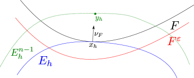
Figure 1: Proof of Proposition 11

This is possible since the minimum is strict. The minimizing property of $E^{h}$ can be written as

$$\operatorname{Per}(E_{h}^{n})+\frac{1}{h}\int_{E_{h}^{n}\Delta E_{h}^{n-1}}\left|d_{E_{h}^{n-1}}\right|\leqslant\operatorname{Per}(E^{h}\cap F^{\varepsilon})+\frac{1}{h}\int_{(E^{h}\cap F^{\varepsilon})\Delta E_{h}^{n-1}}\left|d_{E_{h}^{n-1}}\right|.$$

Thus we have, recalling that the flow is monotone since we are dealing with minimizing hulls,

$$\int_{E_{h}^{n-1}\setminus E_{h}^{n}}\left|d_{E_{h}^{n-1}}\right|-\int_{E_{h}^{n-1}\setminus(E^{h}\cap F^{\varepsilon})}\left|d_{E_{h}^{n-1}}\right|\leqslant h(\operatorname{Per}(E^{h}\cap F^{\varepsilon})-\operatorname{Per}(E^{h})).$$

Now, let us notice that since $F^{\varepsilon}$ is a smooth set, we have

$$\operatorname{Per}(E^{h}\cap F^{\varepsilon})=\operatorname{Per}(E^{h};F^{\varepsilon})+\operatorname{Per}(F^{\varepsilon};E^{h})$$

so we can rewrite

$$-\int_{E^{h}\setminus F^{\varepsilon}}\left|d_{E_{h}^{n-1}}\right|\leqslant h(\operatorname{Per}(F^{\varepsilon};E^{h})-\operatorname{Per}(E^{h};(F^{\varepsilon})^{c})).$$ (22)

Finally, we get

$$\int_{E^{h}\setminus F^{\varepsilon}}\left|d_{E_{h}^{n-1}}\right|\geqslant h(\operatorname{Per}(E^{h};(F^{\varepsilon})^{c})-\operatorname{Per}(F^{\varepsilon};E^{h})).$$

Observing that if $\nu^{\varepsilon}$ is the outer normal vector to $F^{\varepsilon}$,

$$\operatorname{Per}(F^{\varepsilon};E^{h})=\int_{\partial F^{\varepsilon}\cap E^{h}}1\ d\mathcal{H}^{n-1}=\int_{\partial F^{\varepsilon}\cap E^{h}}\frac{\nabla\varphi}{|\nabla\varphi|}\cdot\nu^{\varepsilon}\ d\mathcal{H}^{n-1}$$

and if $\nu^{h}$ is the outer normal to $E^{h}$ and $\partial^{\ast}E^{h}$ its reduced boundary, we have

$$\operatorname{Per}(E^{h};(F^{\varepsilon})^{c})=\int_{\partial^{\ast}E^{h}\cap(F^{\varepsilon})^{c}}1\ d\mathcal{H}^{n-1}\geqslant\int_{\partial^{\ast}E^{h}\cap(F^{\varepsilon})^{c}}\frac{\nabla\varphi}{|\nabla\varphi|}\cdot\nu^{h}\ d\mathcal{H}^{n-1}.$$

Plugging into (22) and denoting by $\nu$ the outer normal vector to $E^{h}\setminus F^{\varepsilon}$ ($\nu=\nu^{h}$ on $\partial E^{h}$ and $\nu=-\nu^{\varepsilon}$ on $\partial F^{\varepsilon}$) we have

$$\int_{E^{h}\setminus F^{\varepsilon}}\left|d_{E_{h}^{n-1}}\right|\geqslant h\int_{\partial^{\ast}(E^{h}\setminus F^{\varepsilon})}\frac{\nabla\varphi}{|\nabla\varphi|}\cdot\nu\ d\mathcal{H}^{n-1},$$

which, applying Green’s formula, gives

$$\int_{E^{h}\setminus F^{\varepsilon}}\left|d_{E_{h}^{n-1}}\right|\geqslant\int_{E^{h}\setminus F^{\varepsilon}}h\operatorname{div}\left(\frac{\nabla\varphi}{|\nabla\varphi|}\right).$$

Letting $\varepsilon$ go to zero, we get, at $(x_{h},t_{h})$,

$$\left|d_{E_{h}^{n-1}}\right|\geqslant h\operatorname{div}\left(\frac{\nabla\varphi}{|\nabla\varphi|}\right).$$ (23)

Now, let $y_{h}\in\partial E_{h}^{n-1}$ which realizes the distance between $x_{h}$ and $(E_{h}^{n-1})^{c}$. By construction, we have

$$u_{h}(y_{h},t_{h}-h)=u_{h}(x_{h},t_{h})$$

So, since $(x_{h},t_{h})$ realizes the minimum of $u_{h}-\varphi$, we have

$$\varphi(y_{h},t_{h}-h)\leqslant\varphi(x_{h},t_{h}).$$

Then, let us write

$$\varphi(y_{h},t_{h}-h)=\varphi(x_{h},t_{h})-h\varphi_{t}(x_{h},t_{h})+\nabla\varphi(x_{h},t_{h})\cdot(y_{h}-x_{h})+o(h+x_{h}-y_{h}),$$

we get

$$-h\varphi_{t}(x_{h},t_{h})+\nabla\varphi(x_{h},t_{h})\cdot(y_{h}-x_{h})+o(h+x_{h}-y_{h})\leqslant 0.$$

Since the level sets of $u_{h}$ are minimizing hulls, $u_{h}$ is non decreasing, which implies $\varphi_{t}\geqslant 0$. On the other hand, $\nabla\varphi(x_{h},t_{h})$ must point outside $E^{h}$ so $\nabla\varphi(x_{h},t_{h})\cdot(y_{h}-x_{h})\geqslant 0$. This implies

$$|\nabla\varphi(x_{h},t_{h})|\left|d_{E_{h}^{n-1}}\right|\leqslant h\varphi_{t}.$$

Replacing that into (23), we obtain, at $(x_{h},t_{h})$,

$$\varphi_{t}\geqslant|\nabla\varphi|\operatorname{div}\left(\frac{\nabla\varphi}{|\nabla\varphi|}\right).$$

Since $\varphi$ is smooth and $\nabla\varphi(\hat{x},\hat{t})\neq 0$; we can pass to the limit in $h$ and get a contradiction.

Let us now deal with the case $\nabla\varphi(\hat{x},\hat{t})=0$ and consider the sequence $(x_{h},t_{h})$ constructed as before. Then, either one can find a subsequence $(x_{h_{k}},t_{h_{k}})\to(x,t)$ such that $\nabla\varphi(x_{h_{k}},t_{h_{k}})\neq 0$ or we have for every $h$ sufficiently small, $\nabla\varphi(x_{h},t_{h})=0.$
In the first alternative, note that what we have just done still applies with minor changes. Indeed, we just have to get the contradiction taking the limsup instead of the full limit. The definition of $F^{\ast}$ ensures we keep the inequality.
On the other hand, if $\nabla\varphi(x_{h},t_{h})=0.$ for every small $h$, then we add a term $|x-\hat{x}|^{\alpha}$ (we denote by $\tilde{\varphi}$ the sum), with $\alpha>2$, to $\varphi.$ The first and second derivative of $\varphi$ do not change. If one can find $\alpha$ such that $u_{h}-\tilde{\varphi}$ has a maximum at some $(x_{\alpha}^{h},t_{\alpha}^{h})$ with $\nabla\tilde{\varphi}(x_{\alpha}^{h_{n}},t_{\alpha}^{h_{n}})\neq 0$ for a subsequence $h_{n}\to 0$, then we get the same contradiction. If not, that means that

$$\forall\alpha>2,\quad\nabla\varphi(x_{\alpha}^{h},t_{\alpha}^{h})=\alpha x_{\alpha}^{h}|x_{\alpha}^{h}-x_{0}|^{\alpha-2}$$

for all $h$ sufficiently small, which imposes that $\varphi$, which is smooth, must have a non zero derivative of order $k\leqslant\alpha-1$ at $(\hat{x},\hat{t})$. This is not possible.

∎

4.3 The time-limit is locally minimal

We saw that since $u_{0}$ has minimizing hull level sets, so does $u_{h}(\cdot,t)$ and $u$ is therefore nondecreasing in time (this is true for $u_{h}$). As $u$ is uniformly equicontinuous on each compact set, letting $t$ go to $+\infty$ we have a locally uniform convergence to a limit $u_{\infty}$ which is a viscosity solution of

$$|Du|\operatorname{div}\left(\frac{Du}{|Du|}\right)=0$$

with obstacles $u^{+},u^{-}$, thanks to classical theory of viscosity solutions.

Thanks to [18], Theorem 3.10, one has the following result.

Proposition 12.

Let us assume that $\mathcal{H}^{n-1}(\{u=0\})<\infty.$ Then, there exists a relatively open set $U\subset u^{-1}(s)$ with $H^{n-8-\alpha}(u^{-1}(0)\setminus U)=0$ for all $\alpha>0$, such that $u^{-1}(0)\setminus\Omega$ is an analytic minimal surface in a neighborhood of each point of $U$. Moreover, it is stable and stationary in the varifold sense (classically on $U$).

Note in particular that non empty interior of $u^{-1}(s)$ can occur for only countable many $s$.

4.4 Comparison with mean convex hull

In [21], E. Spadaro is interested in the long time behavior of the discrete scheme (16) but with a step $h$ which remains fixed. In this short subsection, we prove that if $\{u=0\}$ does not fatten, then our approach and Spadaro’s build the same surface. The dimension of the ambient space $n$ is assumed to be less or equal to 7. Here are the theorems he gets:

Theorem 3 (Spadaro, [21]).

Let $\Omega\subset\mathbb{R}^{n}$, $n\leqslant 7$, be a $\mathcal{C}^{1,1}$ closed set and $E_{0}\supset\Omega$ a minimizing hull. Then, for a fixed $h$, the iterative scheme (16) converges in time to some limit $E_{\infty}^{h}$. In addition, the $E_{\infty}^{h}$ converge monotonically to some $E_{\infty}$ which satisfies

• $E_{\infty}$ is $\mathcal{C}^{1,1}$,

• $E_{\infty}$ is a minimizing hull,

• $\partial E_{\infty}\setminus\Omega$ is a (smooth) minimal surface.

In addition, Spadaro uses this construction starting from $E_{0}$ with obstacles $\Omega_{\varepsilon}:=\{x\in\mathbb{R}^{n}\,|\,d(x,\Omega)\leqslant\varepsilon\}$ to build a limit $E_{\infty}^{\varepsilon}.$

Theorem 4 (Spadaro).

The set

$$\Omega^{\text{mc}}:=\bigcap_{\varepsilon>0}~E_{\infty}^{\varepsilon}$$

is the mean convex hull of $\Omega$. That means

$$\Omega^{\text{mc}}=\bigcap_{\Omega\subset\Theta\in\mathcal{A}}\Theta$$

where $\mathcal{A}$ is the family of $\Theta\in\mathbb{R}^{n}$ such that for every minimal surface $\Sigma$ such that $\partial\Sigma\subset\Theta$, we have $\Sigma\subset\Theta.$

Let us show that $\Omega^{mc}$ agrees with our limit $\{u_{\infty}=0\}.$ Since Spadaro’s work is in low dimension, the open set $U$ in Proposition 12 is the whole $u^{-1}(0)$. Let us assume that $u_{\infty}^{-1}(0)$ does not fatten. Hence, $\partial\{u_{\infty}\leqslant 0\}=\{u_{\infty}=0\}$ and $\{u_{\infty}=0\}\setminus\Omega$ is a minimal hypersurface with boundary in $\Omega$. Using the very definition of the global barrier, we deduce that $\{u\leqslant 0\}\subset\Omega^{mc}$.

Now, recalling that $\Omega^{mc}$ is a minimizing hull, it is in particular mean-convex, so if $v$ is the truncated signed distance function to $\Omega^{mc}$, it is a stationary subsolution of (5). Let us prove that it is also a supersolution. We know that $\partial\Omega^{mc}$ is a minimal surface out of the obstacle, so $v$ satisfies

$$-|\nabla v|\operatorname{div}\left(\frac{\nabla v}{|\nabla v|}\right)=0$$

in the classical sense whenever $v<u^{+}.$ That is exactly saying that $v$ is a supersolution of (5).

Then, the comparison principle (Proposition 1) implies, since $v\leqslant u_{0}$, that $v\leqslant u$ and then $\{u\leqslant 0\}\supset\Omega^{mc}$.

Finally,

$$\{u\leqslant 0\}=\Omega^{mc}$$

and both approaches coincide.

Acknowledgment

I am grateful to Antonin Chambolle for introducing me to this problem, and for fruitful discussions. I would also like to thank Matteo Novaga for the suggestions he made, especially concerning the good framework to tackle this problem, and his interest in this work.
This work was partially supported by the ANR (Agence Nationale de la Recherche) through HJnet project ANR-12-BS01-0008-01.

References

- [1] L. Almeida, A. Chambolle, and M. Novaga. Mean curvature flow with obstacles. Ann. Inst. H. Poincaré Anal. Non Linéaire, 29(5):667–681, 2012.
- [2] Luis Almeida, Patrizia Bagnerini, Abderrahmane Habbal, Stéphane Noselli, and Fanny Serman. Tissue repair modeling. 9:27–46, May 2008.
- [3] Luís Almeida, Patrizia Bagnerini, Abderrahmane Habbal, Stéphane Noselli, and Fanny Serman. A mathematical model for dorsal closure. Journal of Theoretical Biology, 268(1):105, November 2010.
- [4] Fred Almgren, Jean E. Taylor, and Lihe Wang. Curvature-driven flows: a variational approach. SIAM J. Control Optim., 31(2):387–438, 1993.
- [5] Guy Barles, H Mete Soner, and Panagiotis E Souganidis. Front propagation and phase field theory. SIAM Journal on Control and Optimization, 31(2):439–469, 1993.
- [6] Giovanni Bellettini, Matteo Novaga, and Maurizio Paolini. An example of three dimensional fattening for linked space curves evolving by curvature. Communications in partial differential equations, 23(9-10):1475–1492, 1998.
- [7] Samuel Biton, Pierre Cardaliaguet, Olivier Ley, et al. Nonfattening condition for the generalized evolution by mean curvature and applications. Interfaces and Free Boundaries, 10(1):1–14, 2008.
- [8] Kenneth A. Brakke. The motion of a surface by its mean curvature, volume 20 of Mathematical Notes. Princeton University Press, Princeton, N.J., 1978.
- [9] Antonin Chambolle, Massimiliano Morini, and Marcello Ponsiglione. A nonlocal mean curvature flow and its semi-implicit time-discrete approximation. SIAM Journal on Mathematical Analysis, 44(6):4048–4077, 2012.
- [10] Yun Gang Chen, Yoshikazu Giga, and Shun’ichi Goto. Uniqueness and existence of viscosity solutions of generalized mean curvature flow equations. J. Differential Geom., 33(3):749–786, 1991.
- [11] Michael G. Crandall, Hitoshi Ishii, and Pierre-Louis Lions. User’s guide to viscosity solutions of second order partial differential equations. Bull. Amer. Math. Soc. (N.S.), 27(1):1–67, 1992.
- [12] Klaus Ecker and Gerhard Huisken. Interior estimates for hypersurfaces moving by mean curvature. Invent. Math., 105(3):547–569, 1991.
- [13] Tokuhiro Eto, Yoshikazu Giga, and Katsuyuki Ishii. An area minimizing scheme for anisotropic mean curvature flow. Advances in Differential Equations, 17(11/12):1031–1084, 2012.
- [14] L. C. Evans and J. Spruck. Motion of level sets by mean curvature. I. J. Differential Geom., 33(3):635–681, 1991.
- [15] Nicolas Forcadel. Dislocation dynamics with a mean curvature term: short time existence and uniqueness. Differential Integral Equations, 21(3-4):285–304, 2008.
- [16] Y. Giga, S. Goto, H. Ishii, and M.-H. Sato. Comparison principle and convexity preserving properties for singular degenerate parabolic equations on unbounded domains. Indiana Univ. Math. J., 40(2):443–470, 1991.
- [17] Enrico Giusti. Minimal surfaces and functions of bounded variation, volume 80 of Monographs in Mathematics. Birkhäuser Verlag, Basel, 1984.
- [18] Tom Ilmanen, Peter Sternberg, and William P. Ziemer. Equilibrium solutions to generalized motion by mean curvature. J. Geom. Anal., 8(5):845–858, 1998. Dedicated to the memory of Fred Almgren.
- [19] Gwenael Mercier. Continuity results for tv-minimizers. arXiv preprint arXiv:1605.09655, 2016.
- [20] Gwenaël Mercier and Matteo Novaga. Mean curvature flow with obstacles: existence, uniqueness and regularity of solutions. Interfaces Free Bound., 17(3):399–426, 2015.
- [21] E Spadaro. Mean-convex sets and minimal barriers. Preprint, 2011.
- [22] Gilles Thouroude. Homogénéisation et analyse numérique d’équations elliptiques et paraboliques dégénérées. PhD thesis, École polytechnique X, 2012.
- [23] Naoki Yamada. Viscosity solutions for a system of elliptic inequalities with bilateral obstacles. Funkcial. Ekvac, 30(2-3):417–425, 1987.