On the Mechanism of Activated Transport in Glassy Liquids

Abstract

ABSTRACT: We explore several potential issues that have been raised over the years regarding the “entropic droplet” scenario of activated transport in liquids, due to Wolynes and coworkers, with the aim of clarifying the status of various approximations of the random first order transition theory (RFOT) of the structural glass transition. In doing so, we estimate the mismatch penalty between alternative aperiodic structures, above the glass transition; the penalty is equal to the typical magnitude of free energy fluctuations in the liquid. The resulting expressions for the activation barrier and the cooperativity length contain exclusively bulk, static properties; in their simplest form they contains only the bulk modulus and the configurational entropy per unit volume. The expressions are universal in that they do not depend explicitly on the molecular detail. The predicted values for the barrier and cooperativity length and, in particular, the temperature dependence of the barrier are in satisfactory agreement with observation. We thus confirm that the entropic droplet picture is indeed not only internally-consistent but is also fully constructive, consistent with the apparent success of its many quantitative predictions. A simple view of a glassy liquid as a locally metastable, degenerate pattern of frozen-in stress emerges in the present description. Finally, we derive testable relationships between the bulk modulus and several characteristics of glassy liquids and peculiarities in low-temperature glasses.

Keywords: glass transition, supercooled liquids, $\alpha$-relaxation, RFOT theory, nucleation, configurational entropy

I Motivation

The mechanism of activated transport in liquids near the glass transition and its dramatic slowing down with compression and/or cooling remains a subject of controversy. Langer (2014); Biroli and Garrahan (2013) It is also of great interest in applications; understanding the mechanism will allow us to reliably estimate the relaxation barriers in liquids and thus make predictions on the glass-forming ability of specific substances, among many other things.

The present article attempts to clarify several aspects of the “entropic droplet” mechanism of the activated transport, due to Wolynes and coworkers, Kirkpatrick et al. (1989); Kirkpatrick and Wolynes (1987); Xia and Wolynes (2000); Lubchenko and Wolynes (2004) and obtains simple, qualitative expressions for the activation barrier and the cooperativity length for the $\alpha$-relaxation that connect to material properties very explicitly. The argument also delineates the role of local fluctuations in the energetics of the activated transport.

According to the random first order transition (RFOT) theory, liquids undergo a crossover from mainly collisional to activated transport at sufficiently high densities and/or low temperatures.Lubchenko and Wolynes (2003) A thermodynamic signature of the crossover is that the liquid density profile is no longer uniform but, instead, becomes a collection of sharp peaks. Singh et al. (1985); Stoessel and Wolynes (1984); Baus and Colot (1986); Lowen (1990); Rabochiy and Lubchenko (2012); Mézard and Parisi (1999) The peaks correspond to particles vibrating around certain positions in space, analogously to regular, periodic crystals. In contrast with the periodic crystals, the aperiodic structures are however transient, even if long-lived. Mutual reconfiguration between distinct, long-lived aperiodic structures occurs via local activated events. As a result of these local reconfigurations, the liquid flows and the translational symmetry is eventually restored. In kinetic terms, the crossover to activated transport corresponds to a well-developed timescale separation between atomic vibrations and translations. Lubchenko and Wolynes (2003, 2012) Appropriately, in the meanfield limit the crossover corresponds with the kinetic catastrophe of the mode-coupling theory, Kirkpatrick and Wolynes (1987) whereby all translations freeze completely.

Both the long-lived structures and the mutual reconfigurations have been observed, respectively, by neutron scattering Mezei and Russina (1999) and a variety of non-linear spectroscopic methods.Ashtekar et al. (2010); Tracht et al. (1998); Russell and Israeloff (2000); Cicerone and Ediger (1996) The crossover to the activated transport may occur both above or below the fusion temperature, the two extremes corresponding to very strong and very fragile liquids respectively. Lubchenko and Wolynes (2003) In the latter case, a liquid below the crossover is formally supercooled. For generality, we shall call liquids in the activated transport regime glassy, so as to include in the analysis strong liquids that are already in the activated regime but are not technically supercooled.

In the specific scenario by Wolynes and coworkers,Kirkpatrick et al. (1989); Kirkpatrick and Wolynes (1987); Xia and Wolynes (2000); Lubchenko and Wolynes (2004) the activated reconfigurations proceed by a mechanism akin to nucleation, the corresponding free energy profile given by:

$$F(R)=\frac{4\pi}{3}R^{3}\Delta\tilde{f}+4\pi R^{2}\sigma(R).$$ (1)

The bulk driving force $\Delta\tilde{f}$, in equilibrium, is entirely due to multiplicity of alternative aperiodic states: $\Delta\tilde{f}=-T\tilde{s}_{c}$, where $\tilde{s}_{c}$ is the configurational entropy per unit volume. Lubchenko and Wolynes Lubchenko and Wolynes (2004) have clarified this notion using a library construction of aperiodic liquid states, which explicitly shows that although an individual aperiodic state is replaced by an individual state, the reconfiguration itself is still driven by the configurational entropy, which reflects the full ensemble of thermally relevant, distinct aperiodic states. The configurational entropy is the log-number of such thermally relevant states and is a convenient measure of the degeneracy of the liquid free energy landscape. Counting such aperiodic states becomes unambiguous below the crossover, when particle translations and vibrations are timescale-separated and so mutual reconfigurations between the states are technically rare events. The rate of such rare events can be evaluated quantitatively using the transition state theory. Kramers (1940); Frauenfelder and Wolynes (1985); Hänggi et al. (1990)

The quantity $4\pi R^{2}\sigma(R)$ has the formal structure of a surface tension term and accounts for the mismatch penalty between alternative aperiodic structures. Kirkpatrick, Thirumalai, and Wolynes Kirkpatrick et al. (1989) (KTW) pointed out that the free energies of the aperiodic structures are distributed implying that a smooth interface between two such structures would generally distort somewhat to minimize the local free energy. This is because the penalty for small increases in the interface area increases slower with the extent of the deformation than the concomitant stabilization of the bulk free energy. KTW noticed that this situation is analogous to the random-field Ising model (RFIM), in which the Zeeman splittings on separate sites are uncorrelated Gaussian random variables, where the distribution width is $h$. The total field in a region of size $N$ thus scales as $h\sqrt{N}$. Hereby, a smooth interface between spin-up and down domains would distort to stabilize the randomly distributed Zeeman energy. Villain Villain (1985) devised a coarse-graining procedure by which one can estimate the effective surface tension coefficient $\sigma(R)$, in the RFIM, given the curvature $1/R$ of the interface. Assuming that the hyperscaling relation $\alpha=2-\nu D$ (Ref. Goldenfeld, 1992) for the heat capacity and the correlation length holds in the large droplet limit, KTW Kirkpatrick et al. (1989) have fixed the boundary condition for the $\sigma(R)$ renormalization at infinity, $\sigma(\infty)=0$, to arrive at a particularly simple, scale-free relation between the effective surface tension coefficient and the interface curvature:

$$\sigma(R)=\sigma_{0}(a/R)^{1/2},$$ (2)

where the surface tension coefficient $\sigma_{0}$ at the molecular scale $a$ is proportional to the field $h$:

$$\sigma_{0}\propto h.$$ (3)

Xia and Wolynes Xia and Wolynes (2000) (XW) used notions of the classical density-functional theory (DFT) to estimate $\sigma_{0}$ without using adjustable parameters. This estimate leads to dozens of quantitative predictions for distinct glassy phenomena, both classical and quantum, see Refs. Lubchenko and Wolynes, 2007, 2007; Lubchenko, 2012 for reviews and Refs. Wisitsorasak and Wolynes, 2012; Rabochiy and Lubchenko, 2013; Rabochiy et al., 2013; Wisitsorasak and Wolynes, 2013 for subsequent work. Recently, the surface tension coefficient $\sigma_{0}$ has been estimated using standard DFT methods, Rabochiy and Lubchenko (2013) the results consistent with the simpler XW argument. Thus the original fluctuation field $h$, which was introduced by KTW seemingly phenomenologically, would appear to be determined retroactively.

The nuclei of incipient aperiodic states, which evolve according to Eq. (1), have been called entropic droplets Kirkpatrick and Wolynes (1987); Kirkpatrick et al. (1989) to reflect the entropic nature of the driving force for the nucleation. The critical size $R^{\ddagger}$ for an entropic droplet, at which $\partial F/\partial R=0$, is given by

$$R^{\ddagger}=\left(3\sigma_{0}a^{1/2}/2T\tilde{s}_{c}\right)^{2/3},$$ (4)

while the barrier itself is

$$F^{\ddagger}\equiv F(R^{\ddagger})=3\pi\sigma_{0}^{2}a/T\tilde{s}_{c}=2\pi\sigma_{0}a^{1/2}(R^{\ddagger})^{3/2}.$$ (5)

This allows one to write down a simple relationship between the relaxation time and the critical radius:

$$\tau=\tau_{0}\exp\left(\frac{2\pi\sigma_{0}a^{1/2}}{k_{B}T}\,{R^{\ddagger}}^{3/2}\right).$$ (6)

If the aforementioned hyperscaling relation were not assumed to be obeyed, the exponent $3/2$ would be replaced by $2$, however the relation between $\log\tau$ and $R^{\ddagger}$ is still robustly scale-free within the nucleation scenario.

Despite the apparent quantitative success of the entropic droplet picture, the latter is far from being universally accepted, see for instance Refs. Langer, 2014; Biroli and Garrahan, 2013. Several aspects of the scenario appear to be particularly confusing or controversial, which we highlight in what follows.

The free energies of the liquid before and after reconfiguration are on average equal, prompting a question as to what exactly drives the reconfiguration. The entropic driving force in Eq. (1) seems non-standard from the viewpoint of traditional nucleation theory. For instance, because the bulk driving force is entirely entropic while there is an energetic component to the mismatch penalty—in systems other than strictly rigid particles—it may appear that the energy of the system increases after each nucleation event. Clearly this cannot be true in equilibrium in view of energy conservation.

Furthermore, nucleation profile (1) suggests, at a first glance, that the nucleation event will proceed indefinitely toward $R\to\infty$, implying the reconfigurations are not local. Xia and Wolynes Xia and Wolynes (2000) and others Lubchenko and Wolynes (2001) have argued the reconfiguration will be completed when the droplet size reaches a value $R^{*}$ such that $F(R^{*})=0$, which is the value of $F(R)$ prior to the reconfiguration event. The length $R^{*}$ thus gives the size of a cooperative region; consequently one may think of a glassy liquid as a mosaic of regions that are relatively stabilized and are physically separated by relatively strained regions that are similar to interfaces between coexisting phases. (There are also important distinctions, to be discussed below.) Since $R^{*}=2^{2/3}R^{\ddagger}$, one obtains, by Eq. (6), an asymptotic scaling $R^{*}\propto(\log\tau)^{2/3}$ which seems to agree with state-of-the-art simulations on a variety of liquid models Flenner et al. (2014) at the lowest accessed temperatures although generally disagrees with higher temperature data. The latter disagreement is expected since at increasing temperature, activated dynamics are progressively affected by mode-coupling and barrier-softening effects. Lubchenko and Wolynes (2003, 2012) The identification of $R^{*}$ as the equilibrium droplet size implies, however, that the free energy $F(R)$ does not reach a minimum at equilibrium and thus is distinct from the free energy of the system, which begs for further clarification.

In addition, because the fluctuation field $h$ is not determined at the onset of the calculation of the activation barrier—even though it can be eventually estimated—the calculation of the mismatch penalty in Eq. (1) might be regarded as not entirely constructive, even if internally-consistent. Related to this is a simple notion that if there is no field $h$ to begin with, $h=0$, one may superficially deduce that $\sigma=0$, by Eqs. (2) and (3), which is clearly not true since there must be a mismatch penalty between distinct free energy minima. Perhaps for these reasons, many have regarded the nucleation scenario largely as an analogy to the random field Ising model, Yeo and Moore (2012) not a self-contained microscopic picture. Even more extremely, the nucleation picture of the activated transport is often regarded Langer (2014); Bouchaud and Biroli (2004) as a variation on the heuristic arguments of Adam and Gibbs. Adam and Gibbs (1965)

Bouchaud and BiroliBouchaud and Biroli (2004) (BB) have put forth a somewhat different view of the activated transport, though still within the landscape paradigm. In this view, the ensemble of all states of a compact region of size $\xi$ consists of a contribution from the current state and contributions of the full, exponentially large set of alternative structures. As in the library construction, the surrounding of the chosen region is constrained to be static up to vibrational displacement. What sets apart the current state from all the alternative states is that it fits the environment better. The mismatch energy must scale with the region size $N$ sublinearly while the log-number of alternative states scales linearly. Thus the stability of sufficiently small regions—which are smaller than a certain length $\xi$ analogous to $R^{*}$—can be understood thermodynamically in a straightforward manner: The energetic advantage of being in the current state, due to the matching boundary, outweighs the multiplicity of poorer matching, higher energy states. (This is not unlike the stability of a crystal relative to the liquid below freezing.)

The just listed aspects of the Bouchaud-Biroli picture are essentially equivalent to the library construction, and, in particular, with regard to the entropic nature of the driving force for the activated transport. In contrast with the KTW Kirkpatrick et al. (1989) and library construction, Lubchenko and Wolynes (2004) however, the BB scenario is agnostic as to the concrete mechanism of mutual reconfiguration between alternative aperiodic states, other that the reconfigurations must be rare, activated events. In the absence of such a concrete mechanism, BB end up assuming a generic scaling relation between the cooperativity length $\xi$ and relaxation time that is similar to Eq. (6); the exponent is generally different from $3/2$, but necessarily positive. In this view, a region larger than the size $R^{*}$ can still reconfigure via a single activated event but would do so typically more slowly than the region of size $R^{*}$. Combining this notion with the lower bound on the cooperativity size obtained above one concludes that the cooperativity size is in fact $R^{*}$ and one does not face the subtlety stemming from the downhill decrease of the free energy profile $F(R)$ from Eq. (1).

Non-withstanding its elegance, the Bouchaud-Biroli picture does rely on scale-free relations similar to Eqs. (4) and (6), which is not necessarily innocuous. Such scale-free relations would naturally arise if the lengthscale $R^{\ddagger}$ (and $R^{*}\propto R^{*}$) could in principle diverge, which is only possible if the configurational entropy $s_{c}$ could vanish, by Eq. (4). (To avoid confusion, we stress that such vanishing could not be observed in practice, by Eq. (5).) Remarkably, the configurational entropy extrapolated beyond the glass transition temperature would vanish at a finite temperature often denoted as $T_{K}$. The vanishing of the configurational entropy—which is often referred to as the Kauzmann crisis Kauzmann (1948)—has been one of the most disputed topics in the glass transition field. There are mean-field models, such as the celebrated Potts glass, Kirkpatrick and Wolynes (1987) which exhibits both a kinetic catastrophe analogous to the crossover from the collisional to activated transport, and an entropy crisis whereby the degeneracy of the landscape vanishes at a finite temperature. Yet the applicability of mean-field Potts models to liquids has been questioned. Langer (2014) Note however that two recent works have shown finite-dimensional Potts-like models could in fact exhibit the RFOT transition. Chiara Angelini and Biroli (2014); Takahashi and Hukushima (2014) Additionally, spin models have been analyzed that exhibit the kinetic and thermodynamic catastrophes in mean-field, but in finite dimensions, the Kauzmann crisis disappears and no diverging length of the type in Eq. (4) is found. Tarzia and Moore (2007); Yeo and Moore (2012, 2012) Last, but not least, Stevenson and Wolynes Stevenson and Wolynes (2011) have argued that a supercooled liquid will crystallize or partially order before the configurational entropy could vanish.

We stress that in the nucleation scenario, formula (4)—which gratuitously happens to be also a scaling relation—is derived on a microscopic basis; it is not postulated and does not rely in any way on the vanishing of the configurational entropy. For this reason, comparisons with spin models that may or may not experience the Kauzmann crisis are not consequential so long as that the nucleation mechanism is in fact correct. Now, because the KTW and subsequent derivations are quite specific as to the details of the activated event and the value of the surface tension, the nucleation scenario allows one to make not only qualitative, but also, apparently, quantitative predictions for many, seemingly disparate phenomena as already mentioned. To establish whether these successful predictions are not mere coincidences, it is imperative to ascertain whether or not the entropic-droplet picture is in fact fully constructive.

The present work clarifies, we believe, the potential issues listed above, which have been raised with regard to the entropic droplet scenario over the years. We thus confirm the constructive nature of the corresponding microscopic description. The key notion that resolves all of those seeming paradoxes is that, on the one hand, the free energies of the individual free energy minima are distributed. On the other hand, the minima cannot interconvert by means other than the activated reconfigurations themselves. This is in contrast with nucleation of a minority-phase Bray (1994) during regular first order transitions, in which the microstates within individual phases interconvert on time scales much shorter than the duration of the nucleation event. That the free-energy fluctuations in glassy liquids are frozen-in on the time scale of the nucleation event makes all the difference. As part of the argument, we show directly that the original KTW prescription that the local field $h$ be determined by the magnitude of free energy fluctuations is straightforwardly implemented using a standard calculation. The resulting expression for the activation barrier for liquid transport is very simple and confirms the physical view of a glassy liquid as a structurally degenerate pattern of frozen-in free energy fluctuations. Bevzenko and Lubchenko (2009) We believe this expression represents a good zeroth-order estimate of the barrier that possesses a great deal of universality as it boils down to only two parameters reflecting the molecular interactions, viz., the bulk modulus and configurational entropy. Despite its qualitative nature, the argument produces barrier values that are in reasonable agreement with experiment.

The paper is organized as follows: Section II discusses the entropic driving force while Section III revisits the argument for the mismatch penalty. We test the expressions obtained for the barrier against the experiment in Section IV. In Section V, we summarize, derive several scaling relations for glassy liquids, and discuss implications of the present results for certain anomalies observed in cryogenic glasses.

II Glassy liquid as a mosaic made of entropic droplets

We are used to systems whose free energy surface is essentially independent of the system size: For instance, the free energy surface of a macroscopic Ising ferromagnet below its Curie point has two distinct free energy minima that can be distinguished by their average magnetization, which is up or down respectively. If the system is made thrice bigger, the free energy is simply multiplied by a factor of three; that is, while the number of states within each minimum increases exponentially, the number of minima themselves remains the same, i.e., two. In contrast, the number of free energy minima in a glassy liquid scales exponentially with the system size $N$: $e^{s_{c}N}$, where $s_{c}$ is the configurational entropy per particle $s_{c}\equiv\tilde{s}_{c}a^{3}$. Under these circumstances, the system will break up into separate, contiguous regions that are relatively stabilized; the contiguous regions are separated by relatively strained interfaces characterized by a higher free energy density. To see this, suppose the opposite were true and the free energy density were uniform throughout. Owing to the multiplicity of distinct free energy minima, the nucleation rate for another relatively stabilized configuration is finite, as we will see shortly. As a result, the original configuration will be locally replaced by another configuration while the boundary of the replaced region will be relatively strained because of a mismatch between the new structure and its environment. Thus in equilibrium, there is a steady-state concentration of the strained regions; local reconfiguration takes place at a steady rate between distinct aperiodic structures. The concentration of the strained regions and the escape rate from the current liquid configuration can be determined self-consistently, as discussed by Kirkpatrick, Thirumalai, and Wolynes, Kirkpatrick et al. (1989) Xia and Wolynes, Xia and Wolynes (2000) and Lubchenko and Wolynes. Lubchenko and Wolynes (2004)

Here we provide a “microcanonical” version of that argument, which, we hope, will make certain aspects of the nucleation scenario less confusing. We start with the general expression for the partition function of a thermodynamic system in contact with a thermal bath at temperature $T\equiv 1/k_{B}\beta$ and pressure $p$: McQuarrie (1973); Landau and Lifshitz (1980)

$$Z=C\int dEdVe^{-\beta[E+pV-TS(E,V)]}$$ (7)

where $S(E,V)$ is the full entropy of the system as a function of energy $E$ and volume $V$. $C$ is the normalization factor, see below. In the usual manner, the integrand is very small for the smallest values of the energy and volume because of the small number of the corresponding configurations $e^{S(E,V)/k_{B}}$; it is also very small for sufficiently large values of these arguments because of the Boltzmann factor $e^{-\beta(E+pV)}$. For a large enough system size $N$, the integral is dominated by the vicinity of the integrand’s maximum at $E=\overline{E}$, $V=\overline{V}$—which thus correspond to the most likely values of the respective variables—while the probability distribution of the thermodynamic variables is approximately Gaussian:

$$Z = \int\frac{dEdV}{2\pi|\partial^{2}S(E,V)|^{-1}}e^{-\beta[\overline{E}+p\overline{V}-TS(\overline{E},\overline{V})]}$$

$$\times \exp\left[\frac{1}{k_{B}}\left(\frac{1}{2}\frac{\partial^{2}S}{\partial E^{2}}\Delta E^{2}+\frac{\partial^{2}S}{\partial E\partial V}\Delta E\Delta V+\frac{1}{2}\frac{\partial^{2}S}{\partial V^{2}}\Delta V^{2}\right)\right],$$

assuming a well-behaved $S(E,V)$ near $E=\overline{E}$, $V=\overline{V}$. Here, $\Delta E\equiv E-\overline{E}$, $\Delta V\equiv V-\overline{V}$, and $|\partial^{2}S(E,V)|$ is the determinant of the matrix of the second-order derivatives of the entropy with respect to the energy and volume from the argument of the second exponential on the r.h.s. The derivatives are computed at $E=\overline{E}$, $V=\overline{V}$. The first exponential in Eq. (II) is independent of the integration variables and is equal to $e^{-\beta\overline{G}}$, where $\overline{G}\equiv\overline{E}+p\overline{V}-TS(\overline{E},\overline{V}))\equiv\overline{H}-TS(\overline{E},\overline{V}))$ is the equilibrium Gibbs free energy and $\overline{H}$ the enthalpy, of course. By a linear change of variables in the integral, one can determine the magnitude of fluctuation of any thermodynamic quantity of interest; an efficient way to do so is described in Chapter 112 of Ref. Landau and Lifshitz, 1980. Here, we are specifically interested in the fluctuation of the Gibbs free energy:

$$Z=\int\frac{dG}{\sqrt{2\pi\delta G^{2}}}e^{-\beta\overline{G}}\,e^{-(G-\overline{G})^{2}/2\delta G^{2}}.$$ (9)

where $\delta G=\left\langle(G-\overline{G})^{2}\right\rangle^{1/2}$. As shown in the Appendix,

$$\delta G=N^{1/2}\left[\frac{k_{B}TK}{\bar{\rho}}+(K\alpha_{t}-\tilde{s})^{2}\frac{k_{B}T^{2}}{\bar{\rho}\tilde{c}_{v}}\right]^{1/2},$$ (10)

where $K\equiv-V(\partial p/\partial V)_{T}$ is the bulk modulus, $\bar{\rho}\equiv 1/a^{3}$ average particle density, and $\alpha\equiv(1/V)(\partial V/\partial T)_{p}$ thermal expansion coefficient. The quantities $\tilde{c}_{v}$ and $\tilde{s}$ are, respectively, the heat capacity at constant volume and entropy, both per unit volume.

Let us now consider a liquid below the crossover to activated transport but above the glass transition; the liquid is thus equilibrated. Below the crossover, the reconfigurations are rare events compared with vibrational relaxation, which amounts to a well-developed time scale separation between translations and vibrations. This time-scale separation takes place in ordinary liquids at viscosities of order $10$ Ps. Lubchenko and Wolynes (2003, 2012) Because of it, the entropy of the liquid can be written as a sum of distinct contributions:

$$\overline{G} = \overline{H}_{i}-T\overline{S}_{{\mbox{\scriptsize vibr}},\,i}-TS_{c}$$ (11)

$$\equiv \overline{G}_{i}-TS_{c}(\overline{G}_{i}),$$ (12)

where $H_{i}$ is the enthalpy of an individual aperiodic state per particle, while the total entropy is presented here as the sum of the vibrational and configurational contributions, the configurational contribution taking care of particle translations. The subscript “$i$” refers to “individual” metastable aperiodic states. The quantity $\overline{G}_{i}\equiv\overline{H}_{i}-T\overline{S}_{{\mbox{\scriptsize vibr}},\,i}$ would be the Gibbs free energy of the sample if the particles were not allowed to reconfigure but were allowed to vibrate only. It is interesting that the free energy of liquid was written in the form similar to Eq. (12) already in 1937 by Bernal, Bernal (1937) who apparently assumed that molecular vibrations and translations were distinct motions at any temperature, even though this notion is well-justified only below the crossover.

Of direct interest is the distribution not of the full free energy $G$ but that of the free energy $G_{i}$ of individual metastable states:

$$Z=\int\frac{dG_{i}}{\sqrt{2\pi\delta G_{i}^{2}}}e^{S_{c}(\overline{G}_{i})/k_{B}-\beta\overline{G}_{i}}\,e^{-(G_{i}-\overline{G}_{i})^{2}/2\delta G_{i}^{2}}.$$ (13)

The corresponding width of the distribution, $\delta G_{i}\equiv\left\langle(G_{i}-\overline{G}_{i})^{2}\right\rangle^{1/2}$, can be evaluated similarly to $\delta G$ from Eq. (10), see the Appendix:

$$\delta G_{i}= N^{1/2} \left\{\left[K-T\left(\frac{\partial S_{c}}{\partial V}\right)_{T}\right]^{2}\frac{k_{B}T}{K\bar{\rho}}\right.$$ (14)

$$+ \left.[K\alpha_{t}+(\Delta\tilde{c}_{v}-\tilde{s}_{\mbox{\scriptsize vibr}})]^{2}\frac{k_{B}T^{2}}{\bar{\rho}\tilde{c}_{v}}\right\}^{1/2},$$

where $\Delta\tilde{c}_{v}\equiv T(\partial\tilde{s}_{c}/\partial T)_{V}$ is the configurational heat capacity at constant volume and $\tilde{s}_{\mbox{\scriptsize vibr}}$ the vibrational entropy, both per unit volume.

It is convenient, for the present purposes, to shift the energy reference so that $\overline{G}_{i}=0$:

$$Z=\int\frac{dG_{i}}{\sqrt{2\pi\delta G_{i}^{2}}}e^{S_{c}/k_{B}}e^{-G_{i}^{2}/2\delta G_{i}^{2}}.$$ (15)

This way, the partition function gives exactly the number $e^{S_{c}/k_{B}}$ of the (thermally available) states that is not weighted by the Boltzmann factor $e^{-\beta\overline{G}_{i}}$.

Consider now a local region that is currently not undergoing a structural reconfiguration. Because the region is certainly known not to be reconfiguring, its free energy—up to finite-size corrections—is equal to $G_{i}$, which is typically higher than the equilibrium free energy $\overline{G}$ from Eq. (12). The free energy difference $\overline{G}-\overline{G}_{i}=-TS_{c}<0$ is the driving force for the eventual escape from the current structure, and, hence, relaxation toward equilibrium. Next we estimate the actual rate of escape and the typical region size that will have reconfigured as a result of the escape event.

We specifically consider escape events that are local. Therefore, the environment of a chosen compact region is static, up to vibration. Consider the partition function for a compact region of size $N$ surrounded by such a static, aperiodic lattice. The vast majority of the configurations do not fit the region’s boundary as well as the original configuration, and so there is a free energy penalty $\Gamma_{i}>0$ due to the mismatch between the static boundary and any configuration of the region other than the original configuration. We anticipate that since local replacement of a structure amounts to a legitimate fluctuation, $\Gamma$ and $\delta G_{i}$ should be intrinsically related, which will indeed turn out to be the case.

In the presence of the mismatch penalty, the density of states can be obtained by replacing $\overline{G}_{i}\to\overline{G}_{i}+\Gamma$ under the integral in Eq. (13), where $\Gamma\equiv\overline{\Gamma}_{i}$ is the typical value of the mismatch. The latter generally scales with the region size:

$$\Gamma=\gamma N^{x},$$ (16)

but in a sub-thermodynamic fashion: $x<1$, where the coefficient $\gamma(N\to\infty)=\text{const}$. Thus we obtain for the total number of thermally available states for a region embedded in a static lattice:

$$Z=\int\frac{dG_{i}}{\sqrt{2\pi\delta G_{i}^{2}}}e^{S_{c}/k_{B}-\beta\Gamma}e^{-(G_{i}-\Gamma)^{2}/2\delta G_{i}^{2}},$$ (17)

where we set the expectation value of the free energy in the absence of the penalty at zero, as before. (The expectation value of $G_{i}$ corresponding to Eq. (17) is not zero at $N>0$.) Note the argument of the first exponential on the r.h.s. is independent of $G_{i}$ but does depend on the region size $N$, and so does the total number of thermally available states $Z$:

$$Z(N)=e^{s_{c}N/k_{B}-\beta\gamma N^{x}},$$ (18)

where $s_{c}\equiv S_{c}/N$ is the configurational entropy per particle.

Because of the sub-linear $N$-dependence of the mismatch penalty, the number of thermally available states $Z(N)$ depends non-monotonically on the region size. For small values of $N$, this number decreases with the region size, which is expected since the region is stable with respect to weak deformation such as movement of a few particles. At the value $N^{\ddagger}$ such that $(\partial Z/\partial N)_{N^{\ddagger}}=0$, the number of available stats reaches its smallest value and increases with $N$ for all $N>N^{\ddagger}$. This critical size $N^{\ddagger}$:

$$N^{\ddagger}=\left(\frac{x\gamma}{Ts_{c}}\right)^{\frac{1}{1-x}},$$ (19)

corresponds to the least likely size of a rearranging region, and thus corresponds to a bottleneck configuration for the escape event: Indeed, any state at $N<N^{\ddagger}$ is less likely than the initial state and so cannot be a final state upon a reconfiguration; such final state must thus be at $N>N^{\ddagger}$. On the other hand, to move any number of particles $N$ in excess of $N^{\ddagger}$, one must have moved $N^{\ddagger}$ particles as an intermediate step.

The size $N^{*}>N^{\ddagger}$ such that

$$Z(N^{*})=1$$ (20)

is special in that the region of this size has a thermally available configuration, other than the original one, even though the boundary is fixed. By construction, this configuration is mechanically (meta)stable. This implies that a region of size $N^{*}$:

$$N^{*}=\left(\frac{\gamma}{Ts_{c}}\right)^{\frac{1}{1-x}},$$ (21)

can always reconfigure. What happens physically is that the center of the free energy distribution from Eq. (17) moves to the right with $N$ according to $\gamma N^{x}$ because the mismatch typically increases with the interface area. This alone would lead to a depletion of states that are degenerate with the original state, which is typically at $G_{i}=0$. Yet as $N$ increases, the free energy distribution also grows in terms of the overall area, height, and, importantly, width, as more states become available. For a sufficiently large size $N^{*}$, the distribution is so broad that the region is guaranteed to sample a state at $G_{i}=0$ even though the distribution center is shifted to the right by $\Gamma$. One may say that in such a state, a negative fluctuation in the free energy exactly compensates the mismatch penalty. For this to be typically true, we must have

$$\Gamma(N)=\delta G_{i}(N)\hskip 14.22636pt\text{ at }\hskip 14.22636ptN=N^{*},$$ (22)

where we have emphasized that both $\Gamma$ and $\delta G$ depend on $N$.

Finally note that the physical extent $\xi$ of the reconfiguring region:

$$\left(\frac{\xi}{a}\right)^{3}\equiv\frac{4\pi}{3}\left(\frac{R^{*}}{a}\right)^{3}\equiv N^{*}$$ (23)

yields the volumetric cooperativity length for the reconfigurations.

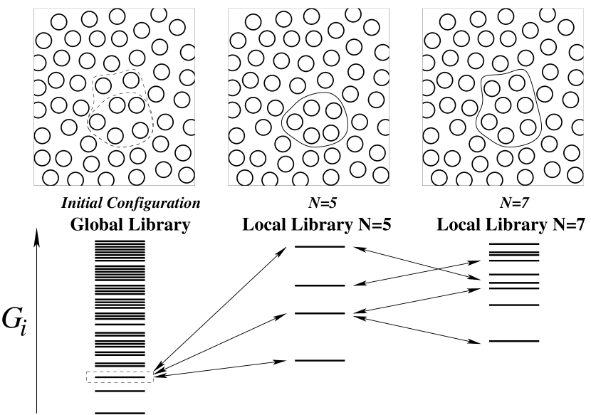
Figure 1: Illustration of the library construction of aperiodic states. Lubchenko and Wolynes (2004) On the left, we start out with some metastable structure. The density of the horizontal bars reflects the increase of the density of states (DoS) $e^{S_{c}(G_{i})/k_{B}}$ with $G_{i}$. This DoS is distinct from the probability distribution in Eq. (17), which also includes the Boltzmann factor $e^{-\beta G_{i}}$. In the center and right panels, 5 and 7 particles have been moved. The density of states pertaining to the corresponding local regions are much lower than the global density of states. In addition, the majority of the thus obtained configurations are higher in free energy than the original configuration, owing to the mismatch with the environment. As the region size grows, the distribution of free energies $G_{i}$ of individual structures is determined by a competition between a depletion due to the mismatch and an entropically-driven increase in the DoS. For a large enough $N=N^{*}$, there will be a configuration whose free energy $G_{i}$ is comparable to that of the original structure.

The above notions can be discussed explicitly in terms of particle movements, within the library construction of aperiodic states, Lubchenko and Wolynes (2004) graphically summarized in Fig. 1. We start out with the original state, which is some state from the full set of states available to the system. We then draw a surface encompassing a compact region containing $N$ particles and consider all possible configurations of the particles inside while the environment is static up to vibration. Most of the resulting configurations are, of course, very high in energy because of steric repulsion between the particles comprising the region itself and between the particles on the opposite sides of the the boundary. Only few configurations will contribute appreciably to the actual ensemble of states, and even those are offset upwards, free energy-wise, by the mismatch penalty. As the chosen region is made progressively bigger, three things happen at the same time: (a) the mismatch penalty typically increases as $\gamma N^{x}$; (b) the log-number of available states first decreases but then begins to increase, asymptotically as $\propto N$; and (c) the spectrum of states becomes broader, the width going as $\propto\sqrt{N}$. Think of (a) as a density of states $e^{S(G_{i})/k_{B}}$ that moves up according to $\gamma N^{x}$ with the region size (see Fig. 1), thus leading to a “depletion” of the density of states at low $G_{i}$. Items (b) and (c), on the other hand, mean the density of states increases in magnitude roughly as $e^{s_{c}N-\Gamma-(G_{i}-\Gamma)^{2}/2\delta G^{2}}$, at fixed $G_{i}$ ($\delta G\propto\sqrt{N}$ and $\Gamma\propto N^{x}$). For a large enough $N$, this growth of the density of states, at fixed $G_{i}$, dominates the depletion due to the mismatch penalty and so the free energy of the substituted configuration eventually stops growing and begins to decrease with the region size $N$, after the latter reaches a certain critical value $N^{\ddagger}$. Eventually, at size $N^{*}$, one will typically find an available state that is mechanically stable.

The discussion of the statistical notions embodied in Eqs. (16)-(21) in terms of particle motions helps one to recognize that the full set of configurations in some range $[0,N_{\text{max}}]$ can be sorted out into (overlapping) subsets according to the following protocol: (a) within each subset, every region size is represented at least once and (b) two configurations characterized by sizes $N$ and $(N+1)$ differ by the motion of exactly one particle. The subsets thus correspond to dynamically-connected paths, along each of which particles join the reconfiguring region one at a time. Along each of the dynamically connected paths, one could thus think of the reconfiguration as a droplet growth. A certain path will dominate the ensemble of the paths given a particular final configuration. This dominating path is the one that maximizes the number of states $Z(N)$ from Eq. (18). This is entirely analogous to the Second Law, whereby the equilibrium configurations are those the maximize the density of states.

One may question whether the most likely bottle-neck configuration in the set of all dynamically connected paths leading to the final state at $N^{*}$ is, in fact, as likely as what is prescribed by $Z(N^{\ddagger})$ with $Z(N)$ from Eq. (18). The answer is yes because sampling of all possible shapes and locations for a region of size $N$ is implied in the summation in Eq. (17). By backtracking individual dynamically-connected trajectories from $N=N^{*}$ to $N=0$, we can determine the precise reconfigured region that produces the most likely bottle-neck configuration with probability $Z(N^{\ddagger})$.

Now, for region sizes in excess of $N^{*}$, the number $Z(N)$ of available states exceeds one, implying that, for instance, two distinct metastable configurations are available to a region of size $N$ such that $Z(N)=2$. According to the above discussion, the trajectories leading to these two states are generally distinct, though the probabilities of the respective bottle-neck configurations and the corresponding critical sizes $N^{\ddagger}$ should be comparable.

Structural reconfiguration can be equally well discussed not in a microcanonical-like fashion, through the number of states $Z(N)$, but, instead, in terms of the corresponding free energy $F(N)=-k_{B}T\ln Z(N)$, as was originally done by Kirkpatrick, Thirumalai, and Wolynes. Kirkpatrick et al. (1989) This yields the following activation profile for the reconfiguration:

$$F(N)=\Gamma-Ts_{c}N,$$ (24)

Since we are considering all possible configurations for escape, subject to the appropriate Boltzmann weight, this amounts to locally replacing the original configuration encompassing $N$ particles by the equilibrated liquid while the particles in the surrounding are denied any motion other than vibration. Upon the replacement, the local bulk free energy is typically lowered by $\overline{G}-\overline{G}_{i}=-Ts_{c}N$, hence the driving term $-Ts_{c}N$ in Eq. (24).

The equilibrated liquid is a Boltzmann-weighted average of alternative, metastable aperiodic structures that are mutually distinct and are also generally distinct from the initial configuration. Another way of saying two structures are distinct is that the particles belonging to the structures inside and outside do not fit as snugly—at the interface between the structures—as they do within the respective structures. This is quite analogous to the mismatch between two distinct crystalline polymorphs in contact, such as during a first order transition between the polymorphs. In contrast with a polymorphic transition, the scaling of the mismatch penalty with the area of the interface will turn out to be somewhat complicated, whereby $x\neq(D-1)/D$.

Combining the free energy view with the notion of dynamically connected trajectories, due to the library construction, we conclude that the activation profile in Eq. (24) is also a nucleation profile. Naturally, the bottle-neck configuration corresponding to $N=N^{\ddagger}$ from Eq. (19) thus corresponds to the critical nucleus size. The corresponding barrier is equal to

$$F^{\ddagger}\equiv F(N^{\ddagger})=\gamma\left(\frac{x\gamma}{Ts_{c}}\right)^{\frac{x}{1-x}}(1-x).$$ (25)

This directly shows that the escape rate from a specific aperiodic state is indeed finite.

Yet there is more to the activation profile in Eq. (24). In ordinary theories of nucleation, the nucleus continues to grow indefinitely once it exceeds the critical size, unless it collides with other growing nuclei, as it happens during crystallization, or, for instance, when the supply of the contents for the minority phase runs out, as it happens during fog. This essentially unrestricted growth takes places because this way, the system can minimize its free energy by fully converting to the minority phase. This view is adequate when there are only two free energy minima to speak of and the system converts between those two minima.

However in the presence of an exponentially large number of free energy minima, we must go about the meaning of the $F(N)$ curve more carefully. We must recognize that both the initial and final state for the escape event are individual aperiodic states that are, on average, equally likely. In fact, because we have chosen $G_{i}=0$ as our free energy reference, $F(N)$ gives exactly the log-number (times $-k_{B}T$) of thermally available states to the selected region. As a result, that the free energy $F(N)$ reaches its initial value of zero indicates that a mechanically metastable state is available to escape to. One is accustomed to situations in which the initial and final state for a barrier-crossing event are minima of the free energy, which does not seem to be the case in the above argument. There is no paradox here, however. The quantity $F(N)$ is not the actual free energy of the system. Instead, by construction, it is the free energy under the constraint that the outside of the selected compact region be not relaxing in the usual matter, but, instead, be forced to be in a specific, metastable aperiodic minimum. The monotonic decrease of $F(N)$ at $N=N^{*}$ is trivial in that it simply says the surrounding of the droplet will eventually proceed to reconfigure again and again, as it should in equilibrium. As we already emphasized, the state to which the initial configuration has escaped is perfectly metastable.

We now shift our attention to the energy. Suppose the liquid is composed of particles that are not completely rigid, and so the mismatch penalty has an energetic component. Furthermore, it is instructive to suppose that the penalty is mostly energetic, which is probably the case for covalently bonded substances such as silica or the chalcogenides. Zhugayevych and Lubchenko (2010) At a first glance, the energy of the system appears to grow with each nucleation event, since the driving force in Eq. (24) is exclusively entropic, at equilibrium. Such unfettered energy growth is, of course, impossible in equilibrium. On the contrary, the configurations before and after a reconfiguration are typical and the energy must be conserved, on average. The energy change following a transition must be within the typical fluctuation range, which reflects the heat capacity $C_{V}$ at constant volume and the bulk modulus $K$: Landau and Lifshitz (1980)

$$\delta E=\{k_{B}C_{v}T^{2}-V[T(\partial p/\partial T)_{V}-p]^{2}T/K\}^{1/2}.$$ (26)

Note both $C_{V}$ and $V$ pertain to a single cooperative region. The conservation of energy, on average, means that since one new interface appears following an escape event, an equivalent of one interface must have been subsumed during an event, as emphasized in Ref. Zhugayevych and Lubchenko, 2010.

We thus conclude that the equilibrium concentration of the interface configurations is given by $1/\xi^{3}$ with $\xi$ from Eq. (23), and so a glassy liquid is a mosaic of aperiodic structures, Xia and Wolynes (2000) each of which is characterized by a relatively low free energy density, while the interfaces separating the mosaic cells are relatively stressed regions characterized by excess free energy density due to the mismatch between stabilized regions. This stress pattern is not static, but relaxes at a steady pace so that a region of size $\xi$ reconfigures once per time $\tau$, on average:

$$\tau=\tau_{0}e^{F^{\ddagger}/k_{B}T},$$ (27)

where the pre-exponent $\tau_{0}$ corresponds to the vibrational relaxation time.

Note that the total free energy stored in the strained regions corresponding to the domain walls is equal to $\Gamma(N/N^{*})=Ts_{c}N$, i.e. the enthalpy difference between the liquid and the corresponding crystal at the temperature in question, up to possible differences in the vibrational entropy between the crystal and an individual aperiodic structure.

According to Eqs. (19)-(23), we need to evaluate the exponent $x$ and the coefficient $\gamma$ for the mismatch penalty, to estimate the escape rate and the cooperativity size for the activated reconfigurations, to which we proceed next.

III Mismatch Penalty between Dissimilar Aperiodic Structures: Renormalization of the surface tension coefficient

Because the states on both sides of our interface are aperiodic, the degree of mismatch is distributed. Thus in some places the two structures may fit quite well and so the scaling of the surface energy term $\Gamma$ from Eq. (24) with the droplet size $N$ may be weaker than the $N^{(D-1)/D}$ scaling expected for interfaces separating periodic or spatially uniform phases. The mechanism of this partial lowering of the mismatch penalty is as follows: The number of distinct aperiodic structures available to a sufficiently large region, we remind, scales exponentially with the region size. The free energies $G_{i}$ of individual structures from Eq. (12) are distributed; they are equal on average but differ by a finite amount for any specific pair of aperiodic states. Fluctuations of extensive quantities scale with $\sqrt{N}$ as functions of size $N$. Landau and Lifshitz (1980) (The size $N$ at which the $\sqrt{N}$ scaling sets in can be rather small in the absence of long-range correlations, such as those typical of a critical point.) Thus the free energy difference between the configurations outside and inside scales as $\sqrt{N}$, for two regions of the same size $N$, and could be of either sign. Suppose now, for concreteness, that the configuration on the outer side of the domain wall happens to be lower in free energy than the adjacent region on the inside. Imagine distorting the domain wall so as to replace a small portion of the inside configuration by that from the outside. It turns out the free energy stabilization due to the replacement outweighs the destabilization due to the now increased area of the interface, as we shall see shortly.

Before we proceed with this analysis, it is instructive to discuss why such surface renormalization and the consequent stabilization would not take place during regular discontinuous transitions when one phase characterized by a single free energy minimum nucleates within another phase also characterized by a single free energy minimum. After all, both phases represent superpositions of microstates whose energies are also distributed. Furthermore, there seems to be a direct correspondence between, say, the regular canonical ensemble and the situation described in Eq. (12). Hereby, the free energies $G_{i}$ in Eq. (12) seem to correspond to the energies of the microstates, while the configurational entropy $S_{c}$ seems to correspond to the full entropy in the canonical ensemble. One difference between the situation in Eq. (12) and the canonical ensemble is that in the latter, transitions between the microstates within individual phases occur on times much shorter than the observation time or mutual nucleation and nucleus growth. As a result, the energies of the phases on the opposite sides of the interface are always equal to their average values. In contrast, the distinct aperiodic states from Eq. (12) are long-lived. In fact, the fastest way to inter-convert between those states is via creation of the very interface we are discussing! In the canonical ensemble analogy, this would correspond to having individual microstates on the opposite sides of the interface as opposed to ensembles resulting from averaging over all microstates (with corresponding Boltzmann weights). Conversely, the situation in Eq. (12) would be analogous to the canonical ensemble only at sufficiently long times that much exceed the nucleation time from Eq. (27). Note that at such long times, we have identical, equilibrated liquid on both sides and so there is no surface tension in the first place.

Now, the situation where the system can reside in long-lived states whose free energies are distributed in a Gaussian fashion can be equivalently thought of as a perfectly ergodic, equilibrated system in the presence of a static, externally-imposed random field whose fluctuations scale in the Gaussian fashion. In the absence of this additional random field, the mismatch penalty between such two regular phases would be perfectly uniform along an interface with spatially uniform curvature. The simplest system one can think of, in which this situation is realized, is the random field Ising model:

$${\cal H}=-J\sum_{i<j}\sigma_{i}\sigma_{j}-\sum_{i}h_{i}\sigma_{i},\hskip 28.45274pt\sigma_{i}=\pm 1,$$ (28)

where $J>0$ while the Zeeman splittings $h_{i}$’s are random, Gaussianly distributed variables. In the Hamiltonian above, if one were to impose a strictly flat interface between two domains with spins up and down, the domain wall would distort some to optimize the Zeeman energy. However, the amount of distortion is also subject to the tension of the interface between the spin-up and spin-down domains. The overall lowering of the free energy, due to the interface distortion, corresponds to the optimal compromise between these two competing factors. Likewise, a smooth interface between two distinct aperiodic states will distort to optimize with respect to local bulk free energy, which is distributed. The energy compensation will scale, again, as the square root of the variation of the volume swept by the interface during the distortion. The final shape of the interface will be determined by the competition between this stabilization and the cost of increasing the area of the interface.

The mapping between the random field Ising model and large scale fluctuations of the interface between aperiodic liquid structures was exploited by Kirkpatrick, Thirumalai, and Wolynes (KTW) Kirkpatrick et al. (1989), who used Villain’s argument Villain (1985) for the renormalization of the surface in RFIM to deduce how the droplet interface tension scales asymptotically with the droplet size. The mapping relies crucially on the condition that the undistorted interface must not be too thick, as it would be near a critical point. This assumption turns out to be correct since the width of the undistorted interface is on the order of the molecular length $a$. Rabochiy and Lubchenko (2013)

Let us now consider a variation on the KTW-Villain argument concerning the surface tension renormalization. This argument produces the sought scaling relation for the mismatch penalty but some of its steps are only accurate up to factors of order one, and so the latter will be dropped in the calculation. All lengthscales will be expressed in terms of the molecular length $a$, which simply sets the units of length. Now, consider two dissimilar aperiodic states in contact, and assume we have already coarse-grained over all length-scales less than $r$, while explicitly forbidding interface fluctuations on greater lengthscales. The interface is thus taut. Further, consider spatial variations in the shape of the interface on lengthscales limited to a narrow interval $[r,r(1+\Delta)]$. The dimensionless increment

$$\Delta=d\ln r$$ (29)

is the increment of the running argument for our real-space coarse-graining transformation $r\to r(1+\Delta)$. (Ultimately, $r$ will be set at the droplet radius). We may assume, without loss of generality, that the mismatch penalty may be written in the following form, in $D$ spatial dimensions:

$$\Gamma=\sigma(r)r^{D-1},$$ (30)

The quantity $\sigma(r)$ may be thought of as a renormalized surface tension coefficient, where the amount of renormalization generally depends on the wavelength, which is distributed in the (narrow) range between $r$ and $r(1+\Delta)$. Our task is to determine under which condition such renormalization takes place, if any.

To do this, let us deform the interface so as to create a bump of (small) height $\zeta$ and lateral extent $r$. Because the interface is taut, the area will increase quadratically with $\zeta$. The resulting increase in the interface area will incur a free energy cost

$$\delta F_{s}\sim\sigma(r)r^{D-1}(\zeta/r)^{2}\Delta,$$ (31)

when $\zeta\ll r$. It will turn out to be instructive to use a more general form

$$\delta F_{s}\sim\sigma(r)r^{D-1}(\zeta/r)^{z}\Delta.$$ (32)

This generalized form is convenient because (a) rough interfaces may exhibit a $z$ other than $2$ (b) the scaling of the interface tension with $r$ will turn out be independent of $z$ at the end of the calculation. Thus the obtained $\sigma$ vs. $r$ scaling can be argued to still apply even to situations when $\zeta/r$ is not necessarily small. (Which it will not be!) Now, as already mentioned, one can always flip a region (of size $N$) at the interface so a to lower its bulk free energy by $\sim h\sqrt{N}$. The resulting bulk free energy gain is thus:

$$\delta F_{b}\sim-h\sqrt{N}\Delta\sim-h(r^{D-1}\zeta)^{1/2}\Delta,$$ (33)

where the constant $h$ is straightforward to estimate in light of our earlier discussion that the bulk stabilization above is the result of fluctuations of the Gibbs free energy. Thus,

$$h\sim\delta G_{i}/\sqrt{N},$$ (34)

with $\delta G_{i}$ from Eq. (14). Properly, we should have written $h^{2}=2(\delta G_{i})^{2}/N$ in Eq. (34) because the bulk free energy stabilization is a difference between two random Gaussian variables, whose distribution widths are $\delta G_{i}$ each, but we have agreed to drop factors of order one in the derivation, see also below.

Finally, one should not fail to identify the stabilization in Eq. (33) with the Bouchaud-Biroli free energy stabilization of a compact region due to matching with its surrounding.

Next we find the value of $\zeta$ that minimizes the total free energy stabilization: $\partial(\delta F_{s}+\delta F_{b})/\partial\zeta=0$, which yields:

$$\zeta\sim(h/\sigma)^{2/(2z-1)}r^{(2z-D+1)/(2z-1)}.$$ (35)

The resulting energy gain per unit area,

$$\min_{\zeta}\{ \delta F_{s}+\delta F_{b}\}/r^{D-1}\sim$$

$$\sim-(h^{z}/\sigma^{1/2})^{1/(z-1/2)}r^{-z(D-2)/(2z-1)}\Delta,$$ (36)

thus represents the renormalization $\delta\sigma(r)$ of the $r$-dependent “surface tension coefficient” that resulted from integrating out degrees of freedom in the $k$-vector range between $1/r$ and $1/(1+\Delta)r$.

The energy gain per unit area from Eq. (III), due to the real-space renormalization in the wavelength range $[r,r(1+\Delta)]$, can be viewed as an iterative relation, by Eq. (29):

$$d\sigma\sim-(h^{z}/\sigma^{1/2})^{1/(z-1/2)}r^{-z(D-2)/(2z-1)}d\ln r.$$ (37)

A quick inspection of this differential equation shows that the surface tension coefficient decreases with $r$. To determine the actual $r$-dependence of $\sigma$, we must decide on the boundary condition $\sigma(r=\infty)\equiv\sigma_{\infty}$. Suppose for a moment that $\sigma_{\infty}>0$, which implies that at sufficiently large distances, the interface width tends to some finite value $l_{\infty}$, however large. This is because the surface tension coefficient of a flat interface between non-matching equilibrated structures goes as $g^{\ddagger}l_{\infty}$, where $g^{\ddagger}$ is the local free energy density excess at the interface. Rowlinson and Widom (1982); Bray (1994) Since the free energy excess per unit volume $g^{\ddagger}$ tends to a finite value $g^{\ddagger}_{\infty}>0$ in the limit of a flat interface, so should $l_{\infty}$, if $\sigma_{\infty}$ is finite. Now, the surface tension coefficient is thus given by the expression

$$\sigma^{2z/(z-1)}(r)=h^{2z/(2z-1)}r^{-z(D-2)/(2z-1)}+\sigma^{2z/(z-1)}_{\infty}.$$

Inserting the above formula in expression (35) yields:

$$\zeta\sim\frac{r^{(2z-D+1)/(2z-1)}}{[r^{-z(D-2)/(2z-1)}+(\sigma_{\infty}/h)^{2z/(2z-1)}]^{1/z}}$$ (38)

The above formula indicates that although incremental changes in the interface curvature following the renormalization are small, the compound increase in the interface thickness—due to the curvature changes in the broad wavelength range spanned by the coarse-graining procedure—is not necessarily so.

Eq. (38) indicates that there are two internally-consistent options regarding the value of the surface tension coefficient $\sigma_{\infty}$. In the conventional case of zero random field, $h=0$, $\sigma_{\infty}$ is finite while $\zeta=0$, and so no renormalization takes place while the interface width tends to a steady value $l_{\infty}$ at diverging droplet radii. If, on the other hand, the random field is present, the only remaining option is $\sigma_{\infty}=0$. Indeed, by Eq. (38), the interface width $\zeta$ diverges as $r\to\infty$, when $h>0$, implying the supposition of a finite $\sigma_{\infty}$ and, hence, finite $l_{\infty}$ was internally inconsistent. For this argument to be valid, the renormalized interface width $\zeta$ should exceed the width $l$ of the original, smooth interface. Condition $\zeta>l$ and Eq. (38), combined with $\sigma_{\infty}=0$, yield

$$r>l,$$ (39)

which happens to coincide with the criterion of validity of the thin interface approximation. Note that in their analysis of barrier softening effects near the crossover, Lubchenko and Wolynes Lubchenko and Wolynes (2003) self-consistently arrived at a similar criterion, viz., $r>a$, for when interface tension renormalization would take place.

It follows that an arbitrarily weak, but finite random field $h$ makes the interface with a sufficiently low curvature unstable with respect to distortion and lowering of the effective surface tension:

$$\sigma(r)\sim\frac{h}{a^{D-1}}(r/a)^{-(D-2)/2},$$ (40)

independent of $z$, apart from a proportionality constant of order one, giving us confidence in the result even when the undulation size $\zeta$ is not very small. Notice we have restored the units of length for clarity.

Eq. (40) yields that the renormalized mismatch energy $\Gamma$ from Eq. (30) scales with the droplet size $N$ is a way that is independent of the space dimensionality, namely $\sqrt{N}$:

$$\Gamma\sim\sigma(r)r^{D-1}\sim h(r/a)^{D/2}\sim h\sqrt{N},$$ (41)

which is ultimately the consequence of the Gaussian distribution of the free energy. Because of the lack of a fixed length scale in the problem—other than the trivial molecular size $a$, which sets the units—it should not be surprising that the interface width $\zeta$ scales with the radius $r$ itself:

$$\zeta\sim r,$$ (42)

again independent of $z$. The numerical constant in the above equation is of order one, as is easily checked, and so $\zeta/r$ is not small generally.

The large effective interface width can be thought of as a result of the distortion of the original thin interface where the extent of the distortion is not determined by a fixed length, but the curvature of the interface itself. In other words, this interface is a fractal object. Because of this fractality, the structure at the interface is not possible to characterize as either of the aperiodic structures on the opposite sides of the original smooth interface before the renormalization. We could thus informally think of this fractal interface as the original thin interface wetted Xia and Wolynes (2000) by other structures that interpolate, in an optimal way, between the two original aperiodic structures. While we are not aware of direct molecular studies with regard to the fractality of cooperative regions in non-polymeric liquids, such studies of polymer melts do suggest the mobile regions are fractal in character.Starr et al. (2013)

According to Eq. (41), the scaling exponent $x$ is equal to $1/2$. Thus the matching condition in Eq. (22) is valid at all values of $N$, while

$$\Gamma=\gamma\sqrt{N},$$ (43)

where $\gamma=\delta G_{i}/\sqrt{N}=\text{const}$, thus yielding:

$$\gamma = \left\{\left[K-T\left(\frac{\partial S_{c}}{\partial V}\right)_{T}\right]^{2}\frac{k_{B}T}{K\bar{\rho}}\right.$$ (44)

$$+ \left.[K\alpha_{t}+(\Delta\tilde{c}_{v}-\tilde{s}_{\mbox{\scriptsize vibr}})]^{2}\frac{k_{B}T^{2}}{\bar{\rho}\tilde{c}_{v}}\right\}^{1/2}.$$

In retrospect, the square-root scaling in Eq. (43) is natural: In view of Eq. (16), the $(G_{i}-\Gamma)^{2}/2\delta G_{i}^{2}$ term under the second exponential in Eq. (17) scales asymptotically with $N$ according to $N^{2x-1}$, see also Ref. Wolynes, 1997. For any $x$ other than $1/2$, this would result in an anomalous scaling Goldenfeld (1992) of the density of states with the system size that would be hard to rationalize given the apparent lack of criticality in actual liquids between the glass transition and fusion temperatures.

Note that the result in Eq. (43)–(44) is only approximate because it does not include finite size corrections. Apart from these corrections, we obtain for the nucleation barrier from Eq. (25):

$$F^{\ddagger}=\frac{\gamma^{2}}{4Ts_{c}}.$$ (45)

Next we estimate $\gamma$. As a rule of thumb, the bulk modulus is about $(10^{1}-10^{2})k_{B}T/\bar{\rho}$ for liquids and $10^{2}k_{B}T/\bar{\rho}$ for solids near the melting temperature $T_{m}$ Bilgram (1987) (consistent with the Lindemann criterion of melting Lindemann (1910); Lubchenko (2006)). The rate of change of the configurational entropy with volume is not known but can be crudely estimated based on the observation that upon freezing, the hard sphere liquid loses $\approx 1.2k_{B}$ worth of entropy per particle while its volume reduces by about $10$%. Hoover and Ree (1968); Hansen and McDonald (1976) Assuming our liquid will run out of configurational entropy at about the same rate—though gradually—we obtain $(\partial S/\partial V)_{T}\sim 10^{1}k_{B}$. Further, $\tilde{s}$ is about $10^{0}k_{B}/a^{3}$. The dimensionless expansivity $\alpha_{t}T$ is generically $10^{-1}$, although could be much smaller for strong substances, see Fig. 12 of Ref. Rabochiy and Lubchenko, 2012. $\Delta\tilde{c}_{v}$ and $\tilde{s}_{c}$ are both $\sim 10^{0}k_{B}/a^{3}$. As a result, we conclude that the volume contribution to the free energy fluctuation in Eq. (14) exceeds the temperature contribution by about two orders of magnitude or so, thus yielding:

$$\gamma^{2}\approx\left[K-T\left(\frac{\partial S_{c}}{\partial V}\right)_{T}\right]^{2}\frac{k_{B}T}{K\bar{\rho}},$$ (46)

since $\bar{\rho}\equiv a^{-3}$.

We thus obtain for the activation barrier:

$$F^{\ddagger}\approx\left[K-T\left(\frac{\partial S_{c}}{\partial V}\right)_{T}\right]^{2}\frac{k_{B}}{4K\tilde{s}_{c}},$$ (47)

where $\tilde{s}_{c}$ is the configurational entropy per unit volume.

According to the above estimate of the $(\partial S_{c}/\partial V)_{T}$ term, it is likely that at least for rigid and weakly attractive particles, the second term in the square brackets is an order of magnitude smaller than the first term. We thus expect the following, simple expression for the surface tension coefficient $\gamma$ to be of comparable accuracy to Eq. (46):

$$\gamma\approx\left(\frac{Kk_{B}T}{\bar{\rho}}\right)^{1/2}\equiv\sqrt{Ka^{3}\,k_{B}T}.$$ (48)

It is interesting that the coefficient $\gamma$ above, which reflects coupling of structural fluctuations to its environment, has exactly the same form as the coupling between the structural reconfigurations corresponding to the two-level systems (TLS) in cryogenic glasses and the phonons. Lubchenko and Wolynes (2001, 2007) Lubchenko and Wolynes have argued the TLS correspond to the two lowest energy levels of the local degrees of freedom that correspond to the low-barrier subset of the activated reconfigurations near the glass transition temperature. Lubchenko and Wolynes (2001, 2007)

The simplified form in Eq. (48) implies for the nucleation barrier:

$$F^{\ddagger}\simeq\frac{K}{4(\tilde{s}_{c}/k_{B})}.$$ (49)

This result can be compared with the earlier expression for the activation barrier derived by Xia and Wolynes, Xia and Wolynes (2000) viz., $F^{\ddagger}=32.k_{B}T/(s_{c}/k_{B})$, in which the configurational entropy is per bead. In contrast, in expression (49) the configurational entropy is per unit volume.

Given that the temperature dependence of the bulk modulus is usually rather weak, Eq. (49) approximately yields the venerable Adam-Gibbs functional relation. Adam and Gibbs (1965) To avoid confusion we emphasize that Eq. (49) applies below the crossover. The Adam-Gibbs relation has also been used to fit temperature dependences of relaxation data above the crossover, but with coefficients that are generally different from those determined in low temperature fits. The presence of a crossover between distinct high-$T$ and low-$T$ Adam-Gibbs behaviors was brought home elegantly by the numerical analysis of Stickel et al.Stickel et al. (1996)

Finally, the expression for the cooperativity size $\xi\equiv a(N^{*})^{1/3}=(\gamma/Ts_{c})^{2/3}$ corresponding to the approximation in Eq. (49) reads:

$$\xi\simeq\left[\frac{K}{k_{B}T(\tilde{s}_{c}/k_{B})^{2}}\right]^{1/3}$$ (50)

Note that neither of the expressions (47), (49), and (50) depends explicitly on the molecular length scale $a\equiv\bar{\rho}^{-1/3}$.

IV Comparison with Experiment and Earlier Approximations

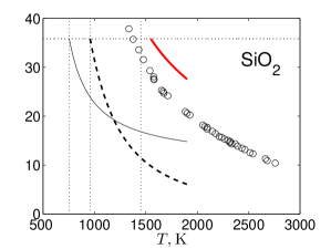
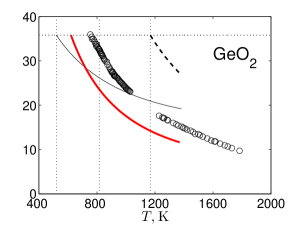
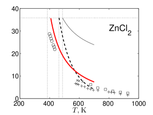
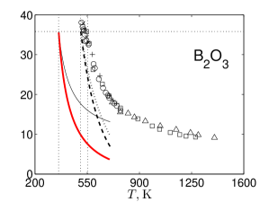
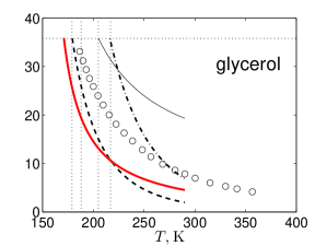
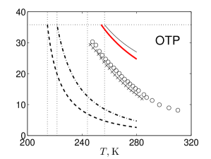
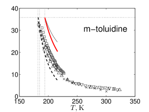
Figure 3: The free energy barrier for $\alpha$-relaxation (divided by $k_{B}T$) as a function of temperature calculated using three approximations. Two earlier approximations, Rabochiy et al. (2013) due to Xia and Wolynes Xia and Wolynes (2000) (XW) and Rabochiy and Lubchenko Rabochiy and Lubchenko (2013) (RL) are shown by the thin solid and thick dashed line respectively. For these calculations, the calorimetric bead count was used. The present approximation is shown with the thick solid red line. The symbols correspond to experimental data; different symbols denote distinct experiments. Because temperature dependences of the structure factor $S(k)$—which is one of the experimental inputs in the RL calculation—are not available, the structure factors measured near $T_{g}$ have been employed. The dash-dotted lines for glycerol and OTP correspond to the RL barrier computed using a higher temperature $S(k)$.

Because the quantity $(\partial S_{C}/\partial V)_{T}$ is not presently available, we analyze the more approximate expression from Eq. (49). As the primary test, we compare the present predictions for the barrier with experiment and two earlier predictions, in relatively extended temperature ranges. These earlier predictions Rabochiy et al. (2013) utilize the values of the surface tension coefficient $\sigma_{0}$ from Eq. (5)—or $\gamma$ from Eq. (45)—as determined by Xia and Wolynes Xia and Wolynes (2000) (XW) and Rabochiy and Lubchenko Rabochiy and Lubchenko (2013) (RL) respectively. We include in the present analysis all eight substances considered in Ref. Rabochiy et al., 2013 except toluene, for which bulk modulus data are not available. The results for the remaining seven substances are shown in Fig. 3. Note that we have estimated the values of the bulk modulus based on the speeds of longitudinal and transverse sound, as determined by Brillouin scattering. The latter procedure yields the adiabatic value of the bulk modulus which somewhat exceeds its isothermal value. It is the isothermal modulus that enters the present estimates. As in Ref. Rabochiy et al., 2013, we have chosen to plot the barriers within the dynamical range representative of actual liquids, viz. $\ln(\tau/\tau_{0})\leq 35.7$, which corresponds to a glass transition on 1 hr time scale and $\tau_{0}=1$ ps. This way, the error of the approximation exhibits itself through an error in the temperature corresponding to a particular value of the relaxation time.

We observe that the present predictions compare reasonably with both experiment and the XW and RL approximations. Although the barrier values predicted with the help of all three approximations are in general agreement with expectation, their deviation from measured values is quite significant for some of the substances. The reader is referred to our earlier detailed discussionRabochiy and Lubchenko (2013); Rabochiy et al. (2013) on the possible sources of error for the elastic constants and the configurational entropy. Also there, the published sources of the experimental data can be found. Here we only note that determination of the elastic constant is affected by a large dissipative component to the elastic response. On the other hand, the estimations of the configurational entropy are subject to uncertainty in the vibrational entropy difference between crystal and glass and the determination of the (putative) Kauzmann temperature by extrapolation of thermodynamic or kinetic data beyond the glass transition temperature.

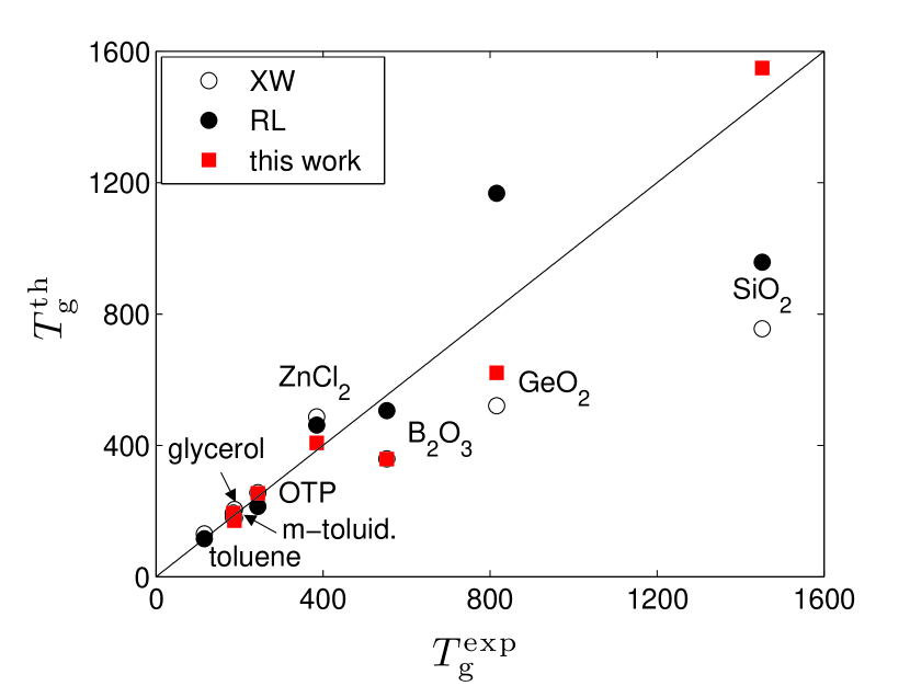
Figure 2: Theoretically predicted glass transition temperatures $T_{g}$, calculated using expression (49), alongside the predictions Rabochiy et al. (2013) utilizing the XW Xia and Wolynes (2000) and RL Rabochiy and Lubchenko (2013) approximations for the mismatch penalty, plotted against experimental values. The theoretically-determined temperatures are based on the barriers from Fig. 3 and rely on static input data, while the experimental values are kinetic quantities obtained from calorimetry.

The results from Fig. 3 can be partially summarized by graphing the predicted values for the glass transition temperature for all three approximations against their experimental values, see Fig. 2. Clearly, theoretical predictions for the glass transition correlate very well with experiment.

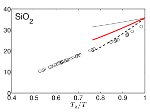
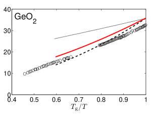
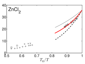
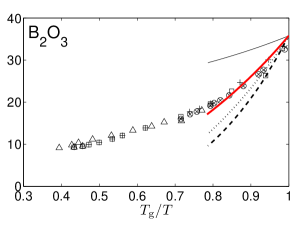
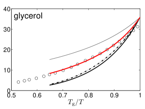
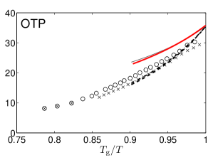
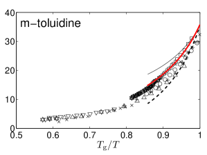
Figure 4: Adjusted barrier for $\alpha$-relaxation (divided by $k_{B}T$) as a function of inverse temperature. The present approximation, from Eq. (49), is multiplied by a constant so as to bring the activation exponent at $T_{g}$, $F^{\ddagger}(T_{g})/k_{B}T_{g}$, to a fixed value of 35.7 (thick solid red line). In the XW (thin solid line) and RL (thick dashed line) approximations, the bead size was determined self-consistently to achieve $F^{\ddagger}(T_{g})/k_{B}T_{g}=35.7$. In all graphs, the temperature is scaled by the experimentally determined $T_{g}$.

Both for the XW and RL calculations, the formulas for the barriers explicitly contain the molecular size $a$. This molecular size is associated with the size of the rigid molecular unit, which we have called the “bead.” The bead size is well-defined for relatively rigid, weakly attractive particles. Lubchenko and Wolynes (2003) In covalently bonded liquids, on the other hand, it can be also understood as the ultra-violet cut-off of the theory. Bevzenko and Lubchenko (2009) In any case, a reasonable estimate for $a$ can be obtained by calibrating the fusion entropy of the substance by that of a Lennard-Jones liquid. Lubchenko and Wolynes (2003); Stevenson and Wolynes (2005) We have called this way to count beads “calorimetric.” Because the uncertainty in the bead size $a$ is potentially a significant contributor to the deviation of the XW and RL predictions from experiment, it is worthwhile to vary it and see whether the deviation can be minimized. This has been done in Ref. Rabochiy et al., 2013 so as to bring the activation exponent $F^{\ddagger}(T_{g})/k_{B}T_{g}$ to a fixed value of 35.7 and results in chemically-reasonable values of $a$, except for OTP. Rabochiy and Lubchenko (2013) The barrier values corresponding to the so renormalized bead size are shown in Fig. 4 for the seven substances in question.

The present predictions, Eqs. (47) and (49), do not depend on the bead size and so the discrepancy with experiment is entirely due to the error in the approximation and in the experimental values of the configurational entropy and the elastic constants. In Fig. 4, we show $F^{\ddagger}(T)/k_{B}T$, with $F^{\ddagger}$ from Eq. (49), multiplied by a constant so as to bring the value of $F^{\ddagger}(T_{g})/k_{B}T_{g}$ to 35.7. We observe that the temperature dependence of the so adjusted barrier is quite similar to experiment, perhaps more so than either of the XW or RL approximation. (We remind that the $T$-dependence of the RL-based barrier values cannot be fully judged based on Figs. 3 and 4 because temperature dependent data for the structure factor are not currently available; as a result the values measured at $T_{g}$ were used.) We note that the experimental value for the $F^{\ddagger}(T_{g})/T_{g}$ ratio is subject to uncertainty in the prefactor $\tau_{0}$ and the cooling rate; the ratio will thus generally differ from 35.7. This, however, is not much of an issue with regard to comparing the slopes of the curves.

Finally we note that the cooperativity length $\xi$ can be straightforwardly computed using Eq. ((50)). The XW and RL based values of $\xi$ are very similar to each other and are close to the experimentally deduced ones in the first place. In view of the similarity of the values of the mismatch penalty computed with the present approximation with those earlier approximations, the cooperativity length (50) is automatically numerically close to those computed in Ref. Rabochiy et al., 2013.

V Discussion and Conclusions

This work has revisited the mechanism of the activated transport in glassy liquids. We have highlighted a key notion that, we hope, will clarify the entropic droplet scenario of the activated transport, due to Wolynes and coworkers. The mutual conversion between metastable (aperiodic) configurations shows an important distinction from mutual conversion between two equilibrated phases, such as during a conventional first order transition. In the latter case, the distribution of the energies of the microstates does not significantly affect the nucleation rate even if the mismatch penalty between the two phases strongly depends on the precise identity of the microstates on the opposite sides of the interface. This is because the microstates within the individual phases interconvert on times scales much shorter than the duration of the nucleation event. As a result, the mismatch penalty between two equilibrium phases is spatially uniform along the interface (of constant curvature) and does not deviate significantly from a certain average value. In contrast, interconversion itself between distinct aperiodic structures is mediated by creation of an interface between those structures. And so the mismatch penalty will strongly depend on the precise identity of the two states separated by the interface; this penalty can be lowered by distorting the interface to give locally a bit more room to that state of the two which is lower in free energy, while not moving the interface as a whole.

The magnitude of the mismatch penalty is essentially equal to the magnitude of local free energy fluctuations. In turn, this magnitude turns out to be straightforwardly related to thermodynamic properties of the liquid, see Eqs. (14) and (44), and is largely determined by the bulk modulus of the liquid. In its most approximate form, the reconfiguration barrier is given by the simplest expression of units energy one could write down, Eq. (49), using the configurational entropy per unit volume and the bulk modulus; note the latter has dimensions energy density. The inverse linear scaling of the barrier with the configurational entropy is special in that it is the only scaling in which the barrier does not explicitly depend on temperature. In turn, this special scaling is a direct consequence of the $\sqrt{N}$ dependence of the mismatch penalty. Interestingly, the barrier does not explicitly depend on the molecular length $a$. To appreciate this, we note that the expression for the cooperativity length $\xi$ does not explicitly contain $a$ either. This is consistent with the mismatch penalty originating from ordinary structural fluctuations which have Gaussian statistics and are scale free. Such fluctuations would not lead to a static heterogeneity, consistent with the results of an independent argument by Cammarota and Biroli. Cammarota and Biroli (2012) In fact, one may think of the mismatch itself as a stress pattern corresponding to frozen-in structural fluctuations or frozen-in stress, consistent with the elasticity-based picture of glassy liquids of Bevzenko and Lubchenko. Bevzenko and Lubchenko (2009)

Although entropic droplet nucleation and mutual nucleation of two coexisting thermodynamic phases are similar in some respects, they also exhibit important differences, including distinct scalings of the mismatch penalty with the droplet size. In addition, during regular first order transitions, the two phases separated by the interface are themselves minima of the free energy of the system. The interfacial configurations may be thought of as corresponding to the barrier that separates the two minima in the bulk term of the Landau-Ginzburg functional that describe the two phases. As a result, the physical space is either wholly occupied by one of the phases or the two phases both occupy macroscopic regions, if they are in near equilibrium. The interfacial configurations thus occupy a negligible portion of the sample. In contrast, the contents of an entropic droplet by themselves do not correspond to a minimum of the free energy. The metastable configuration in the beginning of an activated event ($N=0$) does correspond to a free energy minimum, and so does the configuration at the end of an activated event, upon which a compact region of size $N=N^{*}$ has been replaced by an alternative structure. The border between the reconfigured region and its environment is generally characterized by a higher free energy density. The original configuration also contained similarly strained regions that had resulted from preceding reconfigurations at the locale in question; the energy is thus conserved, on average, as a result of activated events. One may think of a glassy liquid as a mosaic of relatively stabilized regions separated by relatively strained regions. These strained regions can be thought of as transiently frozen-in stress, see Ref. Bevzenko and Lubchenko, 2009 and, also, very recent work by the same authors, Bevzenko and Lubchenko in which alternative procedures of defining the built-in stress are carefully discussed.

The present discussion gives a relatively simple perspective on one of the most intriguing aspects of the structural glass transition: In spin glasses, as in the Sherrington-Kirkpatrick model, Mezard et al. (1987) the disorder is quenched. In contrast, the molecular interactions are translationally invariant and so the disorder in liquids is self-generated. What is the mechanism of this self-generation? The classical density functional theory has shown conclusively that aperiodic structures become metastable at sufficiently high densities.Singh et al. (1985); Stoessel and Wolynes (1984); Baus and Colot (1986); Lowen (1990); Rabochiy and Lubchenko (2012) Within the replica methodologies, Monasson (1995); Mézard and Parisi (1999) one can arrive at the disorder by considering, for instance, a random field generated by a generic boundary for a compact liquid region and then determining this field self-consistently. Within the present discussion, the random field is indeed created by an environment composed of aperiodic structures. The field is effectively static—not unlike the quenched disorder in spin models—but only on the time scale of the activated reconfigurations and thus transiently breaks the translational symmetry.

Because the environment is static, the free energy profile $F(R)$ from Eq. (1)—or $F(N)$ from Eq. (24)—is not the actual free energy of the system. Instead, it gives the log-number (times $-k_{B}T$) of the states thermally available to a chosen compact region under the constraint that its environment be static up to vibration. The value of $F(N)_{N=N^{*}}=0$ is thus special in that it signifies the cooperativity size $N^{*}$ for the reconfigurations because an alternative, mechanically metastable state is available at $N=N^{*}$. The downhill decrease of $F(N)$ at $N=N^{*}$ does not mean that an individual nucleation event will proceed indefinitely past $N^{*}$ but, instead, that the environment itself will eventually proceed to reconfigure. Alternatively, one may think of this downhill decrease as reflecting that more than one aperiodic state with a comparable energy—within the fluctuation range in Eq. (26)—is available to a region of size $N>N^{*}$. The identity of the state to which the liquid will reconfigure is subject to the precise barrier separating that state from the initial configuration. Note that like the bulk free energy of the individual aperiodic states, this barrier is also distributed. The width of this distribution is determined by the configurational heat capacity, which is ultimately responsible for the correlation between the heat capacity jump at the glass transition and the degree of non-exponentiality of liquid relaxations, as established by Xia and Wolynes. Xia and Wolynes (2001) The barrier distribution is also instrumental in the violation of the Stokes-Einstein relation and decoupling between various processes in supercooled liquids. Xia and Wolynes (2001); Lubchenko (2007)

We finish by pointing out several convenient relationships between material constants and various characteristics of the glass transition. For instance, the configurational entropy can be estimated according to the expression:

$$\tilde{s}_{c}=\frac{K}{4T\ln(\tau/\tau_{0})}.$$ (51)

In view of the near universality of $\ln(\tau/\tau_{0})$ at the glass transition, where it is close to 35 or so, we obtain that

$$\tilde{s}_{c}(T_{g})\simeq 10^{-2}\frac{K(T_{g})}{T_{g}}\sim\frac{k_{B}}{a^{3}}.$$ (52)

Likewise, the cooperativity size can be written as

$$\xi^{3}\equiv N^{*}a^{3}=[4\ln(\tau/\tau_{0})]^{2}\frac{k_{B}T}{K},$$ (53)

Again note $\xi$ does not explicitly depend on the molecular length $a$. According to Eq. (53), the cooperative size near the glass transition is on the order of a few hundred rigid molecular units:

$$N^{*}(T_{g})\sim 10^{2}.$$ (54)

Lubchenko and Wolynes Lubchenko and Wolynes (2001, 2007) have argued that the density of states of the two-level systems in cryogenic glasses is approximately equal to $n_{\text{TLS}}\simeq 1/k_{B}T_{g}\xi^{3}(T_{g})$. By Eq. (53), this yields:

$$n_{\text{TLS}}\simeq\frac{K(T_{g})}{[4k_{B}T_{g}\ln(\tau(T_{g})/\tau_{0})]^{2}},$$ (55)

where $K(T_{g})$ is the isothermal bulk modulus just above the glass transition.

Another interesting quantity is the Boson Peak frequency, which has been estimated by Lubchenko and Wolynes Lubchenko and Wolynes (2003) to be about $\omega_{\text{BP}}\simeq(a/\xi)\omega_{D}$, where $\omega_{D}$ is the Debye frequency. This prediction is consistent with experiment. Hong et al. (2011) Using $\omega_{D}\sim c_{s}/a$, we get $\omega_{\text{BP}}\sim c_{s}/\xi$, where $c_{s}$ is the speed of sound. Further noting that $c_{s}\simeq(K/\rho_{M})^{1/2}$, where $\rho_{M}$ is the mass density, and using Eq. (53), we obtain a scaling relation

$$\omega_{\text{BP}}\sim\frac{K^{5/6}(T_{g})}{(k_{B}T_{g})^{1/3}\rho_{M}^{1/2}[4\ln(\tau(T_{g})/\tau_{0})]^{2/3}}.$$ (56)

Lastly, consider the quantity $(\xi/a)^{3}$ that has been argued Lubchenko and Wolynes (2001) to determine the ratio of the phonon mean-free path $l_{\text{mfp}}$ to the the thermal phonon wavelength $\lambda$ in cryogenic glasses. Within the XW approximation, the $(\xi/a)^{3}$ is independent of the bead size $a$ and is universal at $T_{g}$. In the present approximation, this ratio does explicitly depend on $a$ and also on $K$:

$$\frac{l_{\text{mfp}}}{\lambda}\simeq(\xi/a)^{3}=[4\ln(\tau/\tau_{0})]^{2}\frac{k_{B}T_{g}}{K(T_{g})a^{3}}.$$ (57)

In practice, the ratio of the bulk modulus to the glass transition temperature does not vary all that much between different substances because, on the one hand, the $K/T_{m}$ is nearly universal, owing to the Lindemann criterion, while the $T_{m}/T_{g}$ ratio is often numerically near 1.5, even though it does seem to vary between 1.2 and 1.6. As a result, the cooperativity length $\xi$ will exhibit a great deal of universality; the easiest way to vary it in experiment may be to play with the cooling rate at the glass transition. One the other hand, the quantities (55) and (56) scale with energy and are immune to this potential limitation.

Acknowledgments: We are indebted to Peter G. Wolynes for many inspiring conversations. We thank Francesco Zamponi and Simone Capaccioli for sharing fits of the experimental data for the configurational entropy and relaxation times; and also Philip S. Salmon for making available $S(k)$ data for several substances. We gratefully acknowledge the support by the NSF Grant CHE-0956127, the Welch Foundation Grant No. E-1765, and the Alfred P. Sloan Research Fellowship.

Appendix A Fluctuations of the Gibbs free energy

In the Appendix, we will drop the bars over the expectation values of thermodynamical variables, for typographical convenience. In the standard fashion, Landau and Lifshitz (1980) it is convenient to present fluctuations of the Gibbs free energy in terms of fluctuations $\Delta V$ and $\Delta T$ of volume and temperature respectively:

$$\Delta G=\left(\frac{\partial G}{\partial V}\right)_{T}\Delta V+\left(\frac{\partial G}{\partial T}\right)_{V}\Delta T,$$ (58)

which yields

$$\left\langle(\Delta G)^{2}\right\rangle=\left(\frac{\partial G}{\partial V}\right)^{2}_{T}\left\langle(\Delta V)^{2}\right\rangle+\left(\frac{\partial G}{\partial T}\right)^{2}_{V}\left\langle(\Delta T)^{2}\right\rangle,$$ (59)

since $\left\langle\Delta V\Delta T\right\rangle=0$. Landau and Lifshitz (1980) Further using

$$dG=-SdT+Vdp$$ (60)

to compute the derivatives in Eq. (58), the equality Landau and Lifshitz (1980)

$$\left\langle(\Delta V)^{2}\right\rangle=-k_{B}T(\partial V/\partial p)_{T}\equiv k_{B}TV/K,$$ (61)

and the equalities $\left\langle(\Delta T)^{2}\right\rangle=k_{B}T^{2}/C_{v}$, $(\partial p/\partial T)_{V}=-(\partial p/\partial V)_{T}(\partial V/\partial T)_{p}$ one straightforwardly obtains Eq. (10) of the main text.

Analogously for the Gibbs free energy of individual aperiodic states,

$$\Delta G_{i}=\left(\frac{\partial G_{i}}{\partial V}\right)_{T}\Delta V+\left(\frac{\partial G_{i}}{\partial T}\right)_{V}\Delta T.$$ (62)

Eqs. (12) and (60) yield

$$dG_{i}=-S_{\mbox{\scriptsize vibr}}dT+TdS_{c}+Vdp.$$ (63)

Repeating the steps above, one arrives at Eq. (14) of the main text. One should note that Eq. (61) does not apply to solids, in which the shear modulus $\mu>0$. In the latter case, volume fluctuations are of lower magnitude and are given by the expression $\left\langle(\Delta V)^{2}\right\rangle=k_{B}TV/(K+4\mu/3)$. Rabochiy and Lubchenko (2013) Note that here we are dealing with an equilibrated liquid, for which $\mu=0$. Alternatively said, the full distribution of the free energies $G_{i}$ of individual aperiodic states accounts for not only vibrations within individual structures but for the full variety of the structures. Sampling over this variety corresponds to equilibration of the liquid, which corresponds with $\mu=0$.

References

- Langer (2014) Langer, J. S. Theories of Glass Formation and the Glass Transition. Rep. Prog. Phys. 2014, 77, 042501.
- Biroli and Garrahan (2013) Biroli, G.; Garrahan, J. P. Perspective: The Glass Transition. J. Chem. Phys. 2013, 138, 12A301.
- Kirkpatrick et al. (1989) Kirkpatrick, T. R.; Thirumalai, D.; Wolynes, P. G. Scaling Concepts for the Dynamics of Viscous Liquids Near an Ideal Glassy State. Phys. Rev. A 1989, 40, 1045–1054.
- Kirkpatrick and Wolynes (1987) Kirkpatrick, T. R.; Wolynes, P. G. Stable and Metastable States of Mean-Field Potts and Structural Glasses. Phys. Rev. B 1987, 36, 8552–8564.
- Xia and Wolynes (2000) Xia, X.; Wolynes, P. G. Fragilities of Liquids Predicted from the Random First Order Transition Theory of Glasses. Proc. Natl. Acad. Sci. 2000, 97, 2990–2994.
- Lubchenko and Wolynes (2004) Lubchenko, V.; Wolynes, P. G. Theory of Aging in Structural Glasses. J. Chem. Phys. 2004, 121, 2852–2865.
- Lubchenko and Wolynes (2003) Lubchenko, V.; Wolynes, P. G. Barrier Softening Near the Onset of Nonactivated Transport in Supercooled Liquids: Implications for Establishing Detailed Connection between Thermodynamic and Kinetic Anomalies in Supercooled Liquids. J. Chem. Phys. 2003, 119, 9088–9105.
- Singh et al. (1985) Singh, Y.; Stoessel, J. P.; Wolynes, P. G. The Hard Sphere Glass and the Density Functional Theory of Aperiodic Crystals. Phys. Rev. Lett. 1985, 54, 1059–1062.
- Stoessel and Wolynes (1984) Stoessel, J. P.; Wolynes, P. G. Linear Excitations and Stability of the Hard Sphere Glass. J. Chem. Phys. 1984, 80, 4502–4512.
- Baus and Colot (1986) Baus, M.; Colot, J.-L. The Hard-Sphere Glass: Metastability Versus Density of Random Close Packing. J. Phys. C: Solid State Phys. 1986, 19, L135.
- Lowen (1990) Lowen, H. Elastic Constants of the Hard-Sphere Glass: a Density Functional Approach. J. Phys.: Condens. Matter 1990, 2, 8477–8484.
- Rabochiy and Lubchenko (2012) Rabochiy, P.; Lubchenko, V. Universality of the Onset of Activated Transport in Lennard-Jones Liquids With Tunable Coordination: Implications For the Effects of Pressure and Directional Bonding on the Crossover to Activated Transport, Configurational Entropy and Fragility of Glassforming Liquids. J. Chem. Phys. 2012, 136, 084504.
- Mézard and Parisi (1999) Mézard, M.; Parisi, G. Thermodynamics of Glasses: A First Principles Computation. Phys. Rev. Lett. 1999, 82, 747–750.
- Lubchenko and Wolynes (2012) Lubchenko, V.; Wolynes, P. G. In Structural Glasses and Supercooled Liquids: Theory, Experiment, and Applications; Wolynes, P. G., Lubchenko, V., Eds.; John Wiley & Sons, 2012; pp 341–379.
- Kirkpatrick and Wolynes (1987) Kirkpatrick, T. R.; Wolynes, P. G. Connections Between some Kinetic and Equilibrium Theories of the Glass Transition. Phys. Rev. A 1987, 35, 3072–3080.
- Mezei and Russina (1999) Mezei, F.; Russina, M. Intermediate Range Order Dynamics Near the Glass Transition. J. Phys. Cond. Mat. 1999, 11, A341.
- Ashtekar et al. (2010) Ashtekar, S.; Scott, G.; Lyding, J.; Gruebele, M. Direct Visualization of Two-State Dynamics on Metallic Glass Surfaces Well Below . J. Phys. Chem. Lett. 2010, 1, 1941–1945.
- Tracht et al. (1998) Tracht, U.; Wilhelm, M.; Heuer, A.; Feng, H.; Schmidt-Rohr, K.; Spiess, H. W. Length Scale of Dynamic Heterogeneities at the Glass Transition Determined by Multidimensional Nuclear Magnetic Resonance. Phys. Rev. Lett. 1998, 81, 2727–2730.
- Russell and Israeloff (2000) Russell, E. V.; Israeloff, N. E. Direct Observation of Molecular Cooperativity Near the Glass Transition. Nature 2000, 408, 695–698.
- Cicerone and Ediger (1996) Cicerone, M. T.; Ediger, M. D. Enhanced Translation of Probe Molecules in Supercooled -terphenyl: Signature of Spatially Heterogeneous Dynamics? J. Chem. Phys. 1996, 104, 7210–7218.
- Kramers (1940) Kramers, H. A. Brownian Motion in a Field of Force and the Diffusion Model of Chemical Reactions. Physica (Utrecht) 1940, 7, 284.
- Frauenfelder and Wolynes (1985) Frauenfelder, H.; Wolynes, P. G. Rate Theories and Puzzles of Hemeprotein Kinetics. Science 1985, 229, 337.
- Hänggi et al. (1990) Hänggi, P.; Talkner, P.; Borkovec, M. Reaction-rate theory - 50 Years After Kramers. Rev. Mod. Phys. 1990, 62, 251.
- Villain (1985) Villain, J. Equilibrium Critical Properties of Random Field Systems: New Conjectures. J. Physique 1985, 46, 1843.
- Goldenfeld (1992) Goldenfeld, N. Lectures on Phase Transitions and the Renormalization Group; Addison-Wesley, 1992.
- Lubchenko and Wolynes (2007) Lubchenko, V.; Wolynes, P. G. Theory of Structural Glasses and Supercooled Liquids. Annu. Rev. Phys. Chem. 2007, 58, 235–266.
- Lubchenko and Wolynes (2007) Lubchenko, V.; Wolynes, P. G. The Microscopic Quantum Theory of Low Temperature Amorphous Solids. Adv. Chem. Phys. 2007, 136, 95–206.
- Lubchenko (2012) Lubchenko, V. Quantum Phenomena in Structural Glasses: The Intrinsic Origin of Electronic and Cryogenic Anomalies. J. Phys. Chem. Lett. 2012, 3, 1–7.
- Wisitsorasak and Wolynes (2012) Wisitsorasak, A.; Wolynes, P. G. On the Strength of Glasses. Proc. Natl. Acad. Sci. 2012, 109, 16068–16072.
- Rabochiy and Lubchenko (2013) Rabochiy, P.; Lubchenko, V. Microscopic Calculation of the Free Energy Cost for Activated Transport in Glass-Forming Liquids. J. Chem. Phys. 2013, 138, 12A534.
- Rabochiy et al. (2013) Rabochiy, P.; Wolynes, P. G.; Lubchenko, V. Microscopically Based Calculations of the Free Energy Barrier and Dynamic Length Scale in Supercooled Liquids: The Comparative Role of Configurational Entropy and Elasticity. J. Phys. Chem. B 2013, 117, 15204–15219.
- Wisitsorasak and Wolynes (2013) Wisitsorasak, A.; Wolynes, P. G. Fluctuating Mobility Generation and Transport in Glasses. Phys. Rev. E 2013, 88, 022308.
- Lubchenko and Wolynes (2001) Lubchenko, V.; Wolynes, P. G. Intrinsic Quantum Excitations of Low Temperature Glasses. Phys. Rev. Lett. 2001, 87, 195901.
- Flenner et al. (2014) Flenner, E.; Staley, H.; Szamel, G. Universal Features of Dynamic Heterogeneity in Supercooled Liquids. Phys. Rev. Lett. 2014, 112, 097801.
- Yeo and Moore (2012) Yeo, J.; Moore, M. A. Origin of the Growing Length Scale in --Spin Glass Models. Phys. Rev. E 2012, 86, 052501.
- Bouchaud and Biroli (2004) Bouchaud, J.-P.; Biroli, G. On the Adam-Gibbs-Kirkpatrick-Thirumalai-Wolynes Scenario for the Viscosity Increase in Glasses. J. Chem. Phys. 2004, 121, 7347–7354.
- Adam and Gibbs (1965) Adam, G.; Gibbs, J. H. On the Temperature Dependence of Cooperative Relaxation Properties in Glass-Forming Liquids. J. Chem. Phys. 1965, 43, 139–146.
- Kauzmann (1948) Kauzmann, W. The nature of the Glass State and the Behavior of Liquids at Low Temperatures. Chem. Rev. 1948, 43, 219–256.
- Chiara Angelini and Biroli (2014) Chiara Angelini, M.; Biroli, G. The Super-Potts Glass: a New Disordered Model for Glass-Forming Liquids. ArXiv e-prints 2014, http://arxiv.org/abs/1407.7393.
- Takahashi and Hukushima (2014) Takahashi, T.; Hukushima, K. Evidence of One-Step Replica Symmetry Breaking in a Three-Dimensional Potts Glass Model. ArXiv e-prints 2014, http://arxiv.org/abs/1408.1495.
- Tarzia and Moore (2007) Tarzia, M.; Moore, M. A. Glass Phenomenology from the Connection to Spin Glasses. Phys. Rev. E 2007, 75, 031502.
- Yeo and Moore (2012) Yeo, J.; Moore, M. A. Renormalization Group Analysis of the --Spin Glass Model with and . Phys. Rev. B 2012, 85, 100405.
- Stevenson and Wolynes (2011) Stevenson, J. D.; Wolynes, P. G. The Ultimate Fate of Supercooled Liquids. J. Phys. Chem. A 2011, 115, 3713–3719.
- Bray (1994) Bray, A. J. Theory of Phase-Ordering Kinetics. Adv. Phys. 1994, 43, 357–459.
- Bevzenko and Lubchenko (2009) Bevzenko, D.; Lubchenko, V. Stress Distribution and the Fragility of Supercooled Melts. J. Phys. Chem. B 2009, 113, 16337–16345.
- McQuarrie (1973) McQuarrie, D. M. Statistical Mechanics; Harper-Collins, 1973.
- Landau and Lifshitz (1980) Landau, L. D.; Lifshitz, E. M. Statistical Mechanics; Pergamon Press, 1980.
- Bernal (1937) Bernal, J. D. An Attempt at a Molecular Theory of Liquid Structure. Trans. Faraday Soc. 1937, 33, 27–40.
- Zhugayevych and Lubchenko (2010) Zhugayevych, A.; Lubchenko, V. Electronic Structure and the Glass Transition in Pnictide and Chalcogenide Semiconductor Alloys. I: The Formation of the -Network. J. Chem. Phys. 2010, 133, 234503.
- Zhugayevych and Lubchenko (2010) Zhugayevych, A.; Lubchenko, V. Electronic Structure and the Glass Transition in Pnictide and Chalcogenide Semiconductor Alloys. II: The Intrinsic Electronic Midgap States. J. Chem. Phys. 2010, 133, 234504.
- Rowlinson and Widom (1982) Rowlinson, J. S.; Widom, B. Molecular Theory of Capillarity; Clarendon Press: Oxford, 1982.
- Starr et al. (2013) Starr, F. W.; Douglas, J. F.; Sastry, S. The Relationship of Dynamical Heterogeneity to the Adam-Gibbs and Random First-Order Transition Theories of Glass Formation. J. Chem. Phys. 2013, 138, 12A541.
- Wolynes (1997) Wolynes, P. G. Folding Funnels and Energy Landscapes of Larger Proteins within the Capillarity Approximation. Proc. Natl. Acad. Sci. 1997, 94, 6170–6174.
- Bilgram (1987) Bilgram, J. H. Dynamics at the Solid-Liquid Transition: Experiments at the Freezing Point. Phys. Rep. 1987, 153, 1–89.
- Lindemann (1910) Lindemann, F. A. Über die Berechnung molekularer Eigenfrequenzen. Phys. Z. 1910, 11, 609–612.
- Lubchenko (2006) Lubchenko, V. A Universal Criterion of Melting. J. Phys. Chem. B 2006, 110, 18779–18786.
- Hoover and Ree (1968) Hoover, W. G.; Ree, F. H. Melting Transition and Communal Entropy for Hard Spheres. J. Chem. Phys. 1968, 49, 3609–3617.
- Hansen and McDonald (1976) Hansen, J. P.; McDonald, I. R. Theory of Simple Liquids; Academic Press, New York, 1976.
- Stickel et al. (1996) Stickel, F.; Fischer, E. W.; Richert, R. Dynamics of Glass-Forming Liquids. II. Detailed Comparison of Dielectric Relaxation, dc-Conductivity, and Viscosity Data. J. Chem. Phys. 1996, 104, 2043.
- Stevenson and Wolynes (2005) Stevenson, J.; Wolynes, P. G. Thermodynamic-Kinetic Correlations in Supercooled Liquids: A Critical Survey of Experimental Data and Predictions of the Random First-Order Transition Theory of Glasses. J. Phys. Chem. B 2005, 109, 15093–15097.
- Cammarota and Biroli (2012) Cammarota, C.; Biroli, G. Patch-Repetition Correlation Length in Glassy Systems. Europhys. Lett. 2012, 98, 36005.
- (62) Bevzenko, D.; Lubchenko, V. Self-consistent Elastic Continuum Theory of Degenerate, Equilibrium Aperiodic Solids. To appear in J. Chem. Phys., text available on arXiv at http://arxiv.org/abs/1409.7357.
- Mezard et al. (1987) Mezard, M.; Parisi, G.; Virasoro, M. Spin Glass Theory And Beyond; World Scientific, 1987.
- Monasson (1995) Monasson, R. Structural Glass Transition and the Entropy of the Metastable States. Phys. Rev. Lett. 1995, 75, 2847–2850.
- Xia and Wolynes (2001) Xia, X.; Wolynes, P. G. Microscopic Theory of Heterogeneity and Nonexponential Relaxations in Supercooled Liquids. Phys. Rev. Lett. 2001, 86, 5526–5529.
- Xia and Wolynes (2001) Xia, X.; Wolynes, P. G. Diffusion and the Mesoscopic Hydrodynamics of Supercooled Liquids. J. Phys. Chem. 2001, 105, 6570–6573.
- Lubchenko (2007) Lubchenko, V. Charge and Momentum Transfer in Supercooled Melts: Why Should Their Relaxation Times Differ? J. Chem. Phys. 2007, 126, 174503.
- Lubchenko and Wolynes (2003) Lubchenko, V.; Wolynes, P. G. The Origin of the Boson Peak and Thermal Conductivity Plateau in Low Temperature Glasses. Proc. Natl. Acad. Sci. 2003, 100, 1515–1518.
- Hong et al. (2011) Hong, L.; Novikov, V. N.; Sokolov, A. P. Dynamic Heterogeneities, Boson Peak, and Activation Volume in Glass-Forming Liquids. Phys. Rev. E 2011, 83, 061508.