Sharp interface limit for a phase field model in structural optimization
Abstract
We formulate a general shape and topology optimization problem in structural optimization by using a phase field approach. This problem is considered in view of well-posedness and we derive optimality conditions. We relate the diffuse interface problem to a perimeter penalized sharp interface shape optimization problem in the sense of -convergence of the reduced objective functional. Additionally, convergence of the equations of the first variation can be shown. The limit equations can also be derived directly from the problem in the sharp interface setting. Numerical computations demonstrate that the approach can be applied for complex structural optimization problems.
Key words. Shape and topology optimization, linear elasticity, sensitivity analysis, optimality conditions, -convergence, phase field method, diffuse interface, numerical simulations.
AMS subject classification. 35Q74, 35R35, 49Q10, 49Q12, 74B05, 74Pxx.
1 Introduction
In structural optimization one tries to find an optimal material configuration of two different elastic materials in some fixed container, where optimal means that a certain objective functional depending on the behaviour of the elastic materials is minimized. The control here is represented by the material distribution. Applications of shape and topology optimization reach from crashworthiness of transport vehicles and tunnel design to biomechanical applications such as bone remodelling. Structural optimization has turned out to be helpful in solving automative design problems in order to maximize the stiffness of vehicles for instance or to reduce the stresses to improve durability, see for instance [8].
One of the first approaches of finding the optimal material distribution in presence of two materials can be found in [37]. However the problem of finding optimal structures in mechanical engineering dates at least back to the beginning of the 20th century when Michell [32] considered optimal truss layouts. It has turned out, that generally those problems are not well-posed, because oscillations occur on a very fine scale, see for example [9], and hence several ideas have been developed to overcome this issue. One important contribution is certainly the idea of using a perimeter penalization in optimal shape design and considering this problem in the framework of Caccioppoli sets, see [5], in order to prevent the above-mentioned oscillations. Additionally, it turns out that it is difficult to control the state variables if they are only given on varying domains of definitions. And so a so-called ersatz material approach has been introduced, see for instance [2, 16]. Here, one replaces the void regions by a fictitious material which may have a very low stiffness. We also remark that there appear many problems of practical relevance where one wants to fill a given domain with two different materials (and not one material and void) such that after an applied load an objective functional is minimized. Having this in mind it is the main goal of this paper to analyze and numerically solve problems with two materials, whether fictious or not.
We start by stating a perimeter penalized shape optimization problem with a general objective functional in Section 2.2. This is in a simplified form given as
| (1) |
After showing well-posedness we derive necessary optimality conditions by geometric variations without any additional regularity assumption on the minimizing set other than being a Caccioppoli set. This seems to be new as classical shape derivatives always assume at least an open Lipschitz domain as minimizer, see [1, 3, 4, 31], and they do not treat a general objective functional. We also show that the obtained conditions are consistent with existing results obtained with shape derivatives if the minimizing shape inherits a certain regularity.
Then we approximate this problem by using a phase field approach where the free boundary is replaced by a diffuse interface with small thickness related to a parameter . Hence, as in [16], the perimeter functional is replaced by the Ginzburg-Landau energy and the optimization problem reads as
| (2) |
After discussing well-posedness and necessary optimality conditions for the phase field problem we consider the sharp interface limit. To be precise, we show -convergence of the reduced objective functional as the interfacial width, i.e. , tends to zero. Moreover, we show that the equations of the optimality systems converge. We hereby generalize findings from literature where this result has already been indicated in [11] by formal asymptotics for certain objective functionals.
The paper is structured as follows: In Section 2 we introduce the exact problem formulations, discuss well-posedness, optimality conditions and the sharp interface limit. The derivation of the optimality conditions can be found in Section 4 and some proofs of the sharp interface convergence results are collected in Section 5. The numerical approach and results are given in Section 3.
2 Discussion of the problems and convergence results
2.1 Notation and assumptions
Before formulating the shape optimization problems we give a brief introduction into the most important quantities and equations in linearized elasticity and fix some notation. We refer the reader to [17, 18, 24] and references therein for details. We first assume to have in the holdall container two open subsets and which are separated by a hypersurface . The two subsets should correspond to two different elastic materials whose displacement fields are described by one variable . To be precise, corresponds to the displacement field of the -th material where . We divide the boundary of into two parts, one Dirichlet part where we can prescribe the displacement field, and a Neumann part where the applied boundary forces are acting.
-
(A1)
is a bounded Lipschitz domain with outer unit normal and . Moreover, assume with and .
We remark that we denote -valued functions and spaces consisting of -valued functions in boldface.
For elastic materials the following equilibrium constraints hold in , :
| (3a) | |||||
| (3b) | |||||
| (3c) | |||||
where:
-
(A2)
is the given applied surface load, the given applied surface load and for simplicity we assume for the following considerations .
On the interface the boundary conditions are given by certain transmission properties, which follow from . Moreover, is the so-called linearized strain, whereon the linear theory is based and denotes the elastic free energy density of the -th material. We use for , which is in our case independent of . Here, is the elasticity tensor reflecting the material properties for material and , respectively. Further, is the eigenstrain which is given as the value of the strain when the -th material is unstressed. By we denote the derivative with respect to the second component.
As already mentioned above, we have two different elastic materials inside the domain . The design variable is a measurable function , where describes the region where the first material is present up to a set of measure zero, and the region which is filled with the second material. In the sharp interface setting, will only take values in and thus with being the separating hypersurface. In contrast, the phase field approximation uses a design function having values in . Then, where is the diffuse interface of small thickness approximating the hypersurface . Using to describe the sharp as well as the diffuse interface model we describe the elasticity tensor and the eigenstrain as functions of the design variable which interpolate between two different values for the two different materials. We introduce the following assumptions on the elasticity tensor and we use the following assumptions:
-
(A3)
Let be such that fulfills pointwise the following symmetry properties for all . Moreover, we assume that there exist constants such that
(4) holds for all symmetric matrices and .
-
(A4)
Let the eigenstrain be a function with symmetric values, i.e. for all .
Remark 1.
-
1.
The estimates imply that the elasticity tensor interpolates between two finite positive definite tensors, thus in particular no “void”, i.e. regions without material, are allowed in this formulation. Anyhow, the possibility of modelling “void” is given by using the so-called ersatz material approach, where a very soft material approximates the non-presence of material, cf. [11, 16]. Moreover, the elasticity tensor is not depending on the phase field variable introduced later on. Hence, an ersatz material approach depending on the phase field parameter as it is employed in [11] cannot be used in this setting.
-
2.
Following Vegard’s law, a commonly used assumption is that the eigenstrain interpolates linearly between the two values corresponding to the two materials. Then, Assumption (A4) is fulfilled.
Using these assumptions, a weak formulation of the state equations on the whole of can be derived, if the design variable is with a.e. in :
Find such that
| (5) |
In any subregion this yields exactly the weak formulation of . The state equation is in both the phase field and the sharp interface formulation given by , cf. Sections 2.2 and 2.3. Hence we directly state here the solvability result concerning this equation:
Lemma 2.
For every with a.e. in there exists a unique such that is fulfilled. Moreover, the solution fulfills
| (6) |
This defines a solution operator .
Idea of the proof. By making use of Korn’s inequality, this result is a direct consequence of Lax-Milgram’s theorem, cf. [30, Lemma 24.1].
For our shape and topology optimization problem, the goal is to minimize
| (7) |
where fulfill
-
(A5)
and are Carathéodory functions, i.e.
-
1.
and are measurable for each , and
-
2.
are continuous for almost every and , respectively.
Moreover, assume that there exist functions , and , such that it holds
(8) and
(9) Additionally, we assume that the set
is bounded from below.
-
1.
Remark 3.
Due to [36], the Nemytskii operators
are well-defined if and only if and are fulfilled and in this case the operators are continuous.
Assumptions (A1)-(A5) are the basic assumptions for the following considerations. To derive also first order optimality conditions we have to impose at some points additionally the following differentiability assumption.
-
(A6)
For every fixed we have and . Let the partial derivatives exist for almost every and , respectively. Moreover there exist , and , such that
(10) and
(11)
Remark 4.
Under the Assumption (A6) the operators
are continuously Fréchet differentiable and that the directional derivatives are given by , .
In the next remark, we outline how we could replace Assumptions (A5) and (A6) by weaker assumptions. In order to simplify the estimates in the following analysis we prefer (A5) and (A6).
Remark 5.
We could generalise the results to objective functionals satisfying
| (12) |
for some functions and , instead of requiring . Here, has to be chosen such that is a compact imbedding, hence for and for . We then obtain that is well-defined and continuous and all proofs can be adapted. In this case, we have to replace in Assumption (A6) by
for all and a.e. where , to obtain that
is continuously Fréchet differentiable. The same holds for the choice of .
In order to obtain a well-posed problem we add to the cost functional in a regularization term. In the sharp interface problem a multiple of the perimeter of the free boundary between the two materials is used. The exact definition of the perimeter is introduced now. Since we describe the sharp interface model by a design variable , where describe the two different materials, this design variable is going to be a function of bounded variation. We give here a brief introduction in the notation of Caccioppoli sets and functions of bounded variations, but for a detailed introduction we refer to [6, 25]. We call a function a function of bounded variation if its distributional derivative is a vector-valued finite Radon measure. The space of functions of bounded variation in is denoted by , and by we denote functions in having only the values a.e. in . We then call a measurable set Caccioppoli set if . For any Caccioppoli set , one can hence define the total variation of , as is a finite measure. This value is then called the perimeter of in and is denoted by .
We include additionally a volume constraint in the optimization problem. By assuming that the design variable fulfills , which is equivalent to and , for some fixed constant we prescribe a maximal amount of the material corresponding to (and thus a minimal amount of ) that can be used during the optimization process.
Our admissible design variables for the sharp interface problem hence are chosen in the set
| (13) |
In the phase field formulation of the shape optimization problem we approximate the perimeter by the Ginzburg-Landau energy
| (14) |
with a double obstacle potential given by
| (15) |
In the phase field setting, the design variable is allowed to have values in and thus there may be a transition area between the areas and . The admissible set in the phase field setting is given by
| (16) |
and the extended admissible set by
Remark 6.
Instead of we could also use an equality constraint of the form . This prescribes then the exact volume fraction of each material in advance. In this setting, the same analysis can be carried out. The results whereon our sharp interface analysis is based only deal with an equality constraint, see for instance [15, 26, 33].
As we derive first order optimality conditions by varying the free boundary between the two materials with transformations, we introduce here the admissible transformations and its corresponding velocity fields:
Definition 7 (, ).
The space of admissible velocity fields is defined as the set of all , where is some fixed, small constant, such that it holds:
-
(V1)
- (V1a)
-
,
- (V1b)
-
: ,
-
(V2)
for all ,
-
(V3)
for every .
Then the space of admissible transformations is defined as solutions of the ordinary differential equation
| (17) |
with ,
which gives some , with small enough.
We often use the notation .
Remark 8.
We finish this introduction by two typical examples which are commonly used as objective functionals in structural optimization. For a deeper discussion on those problems and some further applications we refer for instance to [8].
Example 9 (Mean compliance).
One commonly used objective in structural optimization is the minimization of the mean compliance, which is for a structure in its equilibrium configuration given by The aim of minimizing this objective functional can be interpreted as maximizing the stiffness under the given forces or as minimizing the stored mechanical energy. We notice, that this is equivalent to minimizing if solves the state equations .
Example 10 (Compliant mechanism).
The typical compliant mechanism objective functional used in topology optimization is given by the tracking type functional where is some desired displacement, and , , is a weighting factor.
In the following, by minimizers we always mean global minimizers.
2.2 Perimeter penalized shape optimization problem
The sharp interface problem that we consider in this section is given by
| (18) |
with such that holds, i.e.
| (19) |
This is a topology and shape optimization problem, where plays the role of the design variable, and can only have the discrete values . The perimeter in the cost functional ensures the existence of a minimizer where the weighting factor can be arbitrary. In the remainder of this subsection we summarize often results where the proofs are given later in this paper or in some previous work. Studying the reduced objective functional ,
we obtain by using the direct method in the calculus of variations the well-posedness of the optimization problem:
Proof.
We use that is equivalent to . According to Assumption (A5), the objective functional is bounded from below and hence we may choose a minimizing sequence for . Thus is uniformly bounded. We obtain therefrom and the fact that for all that is uniformly bounded in . As imbeds compactly into , we hence find that has a subsequence converging in and pointwise to some limit element . From the pointwise convergence we obtain for almost every and the convergence in yields directly . Hence we have . From Lemma 24, which is given in Section 5, we obtain that is continuous in . Moreover, the perimeter functional is lower semicontinuous in , see [6], and thus we obtain . This shows that is a minimizer of , and hence is a minimizer of . ∎
Our next aim is to deduce first order necessary optimality conditions. For this purpose, we use the ideas of shape calculus, which means we apply geometric variations. As already mentioned in the introduction we do not impose any additional regularity assumption on the minimizing set. We obtain:
Theorem 12.
Assume (A1)-(A6). Then for any minimizer of the following necessary optimality conditions hold: There exists a Lagrange multiplier for the integral constraint such that
| (20) |
holds for all with corresponding velocity , where the derivative is given by the following formula:
| (21) |
and
| (22) |
with being the generalised unit normal on the Caccioppoli set , compare [6]. Moreover, is given as the solution of
| (23) |
which has to hold for all .
The proof of this theorem can be found in Section 4.
Remark 13.
If we assume that has -regularity, can be rewritten into a more convenient form by using the identity on .
We can now reformulate those optimality conditions under more regularity assumptions on the minimizing set and the given data. In particular, we can then compare our results to those obtained in literature, see Remark 15.
Theorem 14.
Assume (A1)-(A6). Let be minimizers of . Assume there are open sets such that a.e. on and a.e. in . Let and the objective functional is assumed to be chosen in such a way that and for all . If , we assume additionally that has -regularity. Assume that and . By we denote the jump of along the interface , and is the outer unit normal on . Let be the mean curvature of . Then the optimality conditions derived in Theorem 12 are equivalent to the following system:
| (24) |
| (25) |
together with the state equation connecting and . Here, the adjoint variable is the unique solution of the adjoint equation
| (26) |
The statement of Theorem 14 can be shown by using basic calclations such as integration by parts and chain rule. This calculation has been carried out for instance in [30, Theorem 25.3].
Remark 15.
In [11] the same optimality system for the sharp interface setting has been derived from the phase field model by formally matched asymptotics for the mean compliance and compliant mechanism problems mentioned in Examples 9 and 10. However, no eigenstrain has been taken into account in [11] while this is included in the above problem setting. Applying shape sensitivity analysis yields the same result as we have found in Theorem 14 (see e.g. [1, 4, 31]).
2.3 Phase field approximation
In a diffuse interface setting in terms of a phase field formulation the shape and topology optimization problem of finding the optimal material distribution of two given materials is given by
| (27) |
with such that holds, i.e.
| (28) |
Hence the design variable in this problem is given by . The regions filled with material one or two are represented by and , respectively. The design variable is also allowed to take values between minus one and one, which leads to a small transitional area whose thickness is proportional to a small parameter . Thus, as tends to zero, we will arrive in a sharp interface problem and the interfacial layer vanishes.
As was already discussed in Section 2.1, the Ginzburg-Landau energy , compare , appearing in the objective functional is essential for the existence of a minimizer and -converge to a multiple of the perimeter functional as tends to zero, cf. [33, 34]. The parameter is an arbitrary fixed constant and can be considered as a weighting factor of the perimeter penalization.
We know from Lemma 2 that there is a solution operator for the constraints . Thus, we can reformulate the optimization problem into where ,
is the reduced objective functional. We start by discussing the optimization problem in view of well-posedness for fixed .
Sketch of a proof. Proof of the previous theorem This is established by using the direct method in the calculus of variations. For this purpose, we follow the lines of the proof of Theorem 11. Instead of using the compact imbedding we use here that embeds compactly into and replace the lower semicontinuity of the perimeter functional by the lower semicontinuity of the Ginzburg-Landau energy with respect to convergence in . For more details we refer to [30, Theorem 24.1] or [11], where the case with is treated.
We obtain optimality conditions by geometric variations:
Theorem 17.
Assume (A1)-(A6). Then for any minimizer of the following necessary optimality conditions hold: There exists a Lagrange multiplier for the integral constraint such that
| (29) |
holds for all with corresponding velocity . The derivative is given by the following formula:
| (30) |
where is given as the solution of with replaced by and by . The exact formula for is given in .
The proof can be found in Section 4.
Remark 18.
One can also consider in the framework of optimal control problems. By parametric variations one then obtains as necessary optimality conditions the following variational inequality:
| (31) |
where
| (32) | ||||
is the directional derivative of the reduced objective functional . The variational inequality has to be fulfilled together with the state equations and the adjoint equation . This approach can for instance be used for numerical methods. More details on these optimality criteria can be found in [11, 30].
2.4 Sharp interface limit
In this section we give the results on relating the phase field problems introduced in Section 2.3 to the sharp interface formulation, which was discussed in Section 2.2.
The proof of this theorem is given in Section 5. As a consequence, we obtain directly:
Corollary 20.
Proof.
Theorem 21.
Assume (A1)-(A6). Let be minimizers of . Then there exists a subsequence, which is denoted by the same, that converges in to a minimizer of . Moreover, it holds for all . If then we additionally have the following convergence results:
| (33a) | |||||
| (33b) | |||||
where , and are Lagrange multipliers for the integral constraint defined in Theorem 17, is a Lagrange multiplier for the integral constraint in the sharp interface setting since it fulfills .
The proof is given in Section 5.
3 Numerical experiments
We want to verify the reliability and practical relevance of the phase field approximation by means of numerical experiments. Besides, we also study the behaviour for decreasing phase field parameters and see that the convergence results stated in the previous section are also indicated by numerics. For the numerics, the admissible design functions are chosen in instead of . Thus, the integral volume constraint is replaced by an equality constraint, which means that we prescribe the exact volume fraction in advance. As already discussed in Remark 6, this does not change the analytical results presented in the previous section. The only difference is, that the Lagrange multipliers are also allowed to be negative and the complementarity conditions are fulfilled trivially.
3.1 Description of algorithm
On the reduced problem formulation we apply an extension of the projected gradient method without requiring the existence of a gradient. In addition we allow for a variable scalar scaling of the derivative, as well as the use of a variable metric, which can include second order information. The step length is determined by Armijo backtracking. For more details, see [12, 14].
Algorithm 1.
| (34) |
The maximal number of iterations is set to in the experiments below. The directional derivative is given in . We start with small to enhance the convergence of the PDAS method and increase it slowly in every step until . As an inner product we start choosing . To get faster convergence, we update the inner product in every step by a BFGS update whenever possible. Note that the solution to the projection-type subproblem (34) is formally given by , where denotes the orthogonal projection onto with respect to the inner product and denotes the Riesz representative of with respect to the inner product . This is only formally since need not be differentiable with respect to the norm induced by . The subproblem (34) is solved by a primal dual active set (PDAS) method, see [13, 10].
Remark 22.
In [14] it is shown that every accumulation point of the sequence in the topology is a stationary point of and that . Additionally mesh independence can be observed.
For all of our numerical experiments we consider the compliance problem, see Example 9, and assume to have only the external surface load as well as no eigenstrain, hence and . Thus we choose , . In the following examples will always be an element in and so Assumption (A5) is fulfilled. Thus the objective functional is given in the following numerical experiments by
The used elasticity tensor interpolates between its two values quadratically. Inside the first material (represented by ) and the second material (represented by ) it is given by the two Lamé constants and , respectively. We choose where , thus and , and , .
The phase field and the state equation are discretized using standard piecewise linear finite elements. An adaptive mesh is implemented, which is fine on the interface and coarse in the bulk region as described in [7]. All appearing integrals are computed by exact quadrature rules.
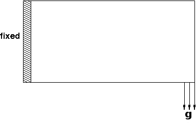
3.2 Optimal design of a cantilever beam
The first experiment is carried out in the design domain and we choose and the support of the force will be concentrated on . The surface load is chosen to be . The configuration is sketched in Figure 1(a) and the initial shape always corresponds to . Thus, also is chosen for the volume constraint. The first material, represented by is given by the constants and the second material (i.e. ) is a more elastic material with . Lamé constants with such a pronounced contrast also appear in applications, compare [35]. A uniform mesh size of is chosen on the bulk and the interfacial layer is refined such that there are 8 mesh points across the interface. Since the interface thickness is proportional to , the mesh has to be chosen finer on the interface as gets smaller.

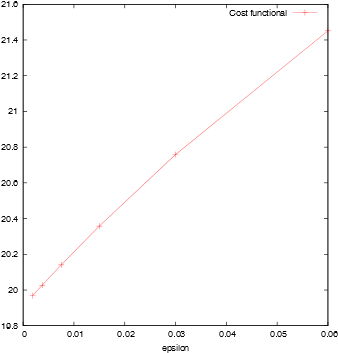 (b) The cost functional seems to converge as .
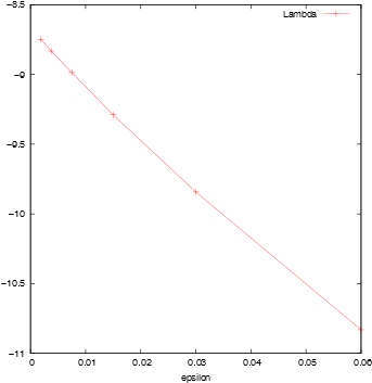 (c) The Lagrange multiplier seems to converge as .
|
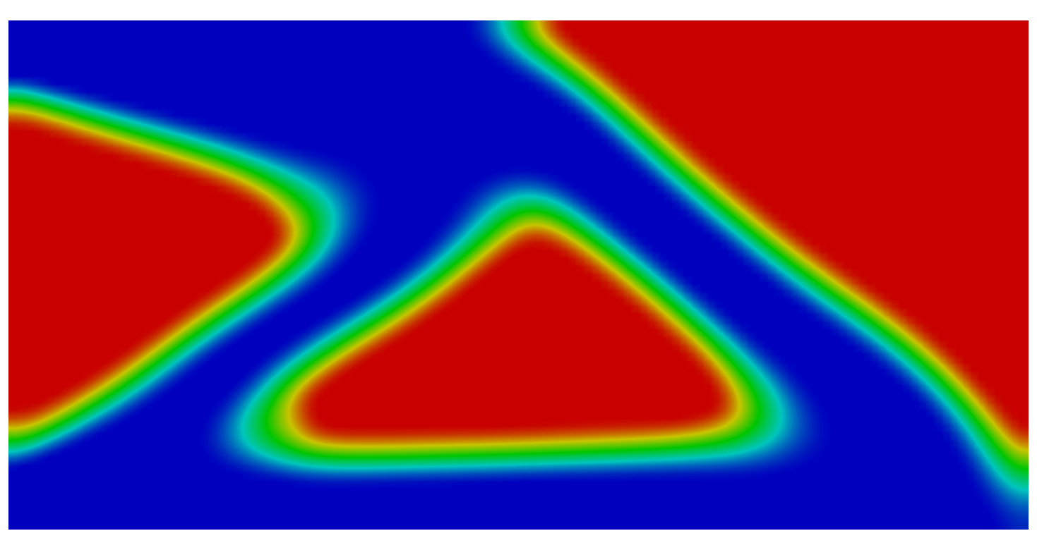
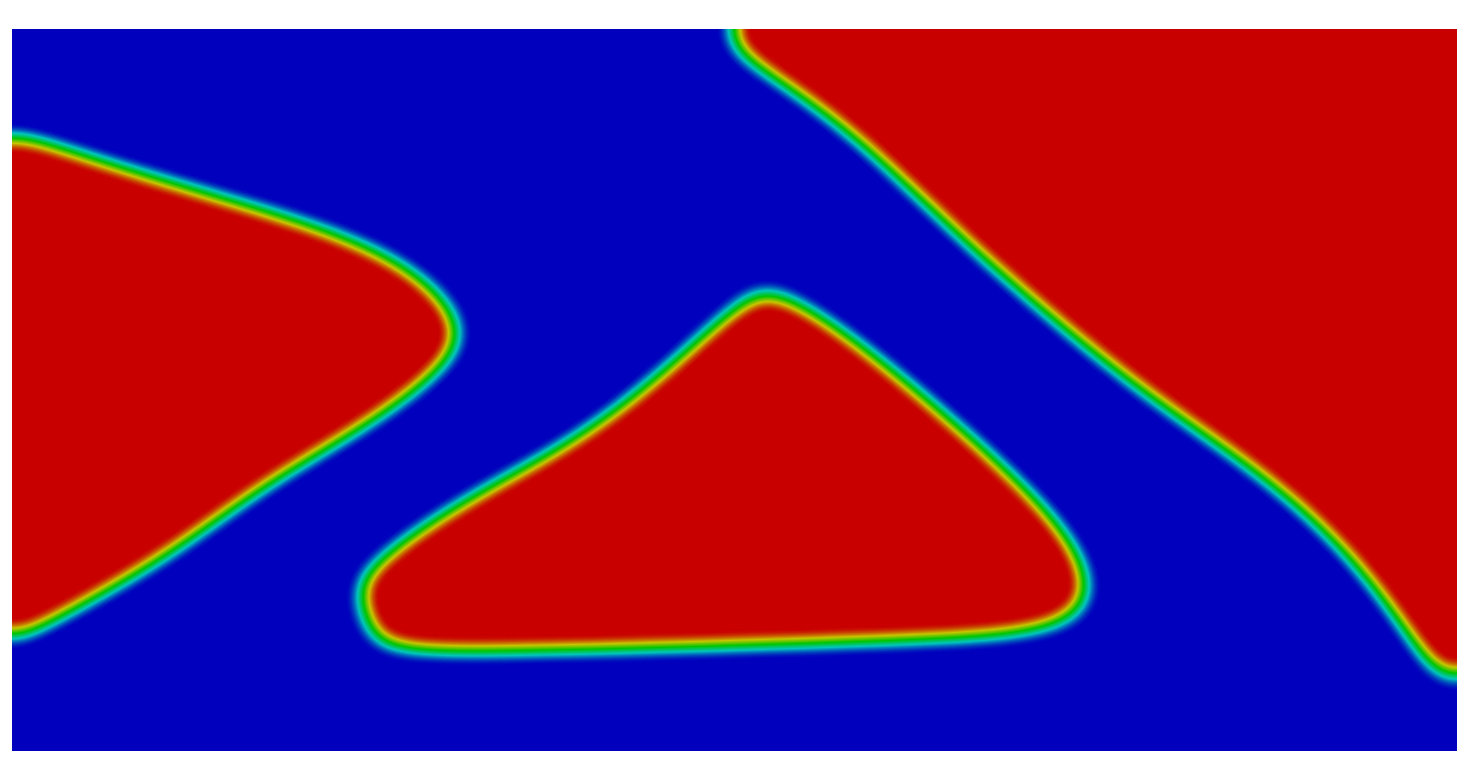
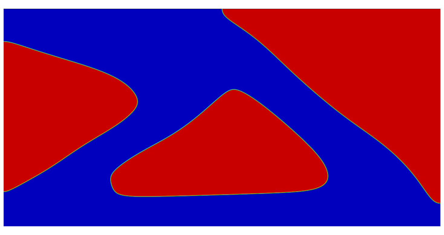
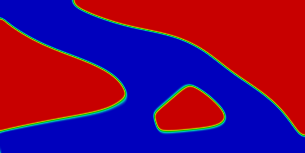
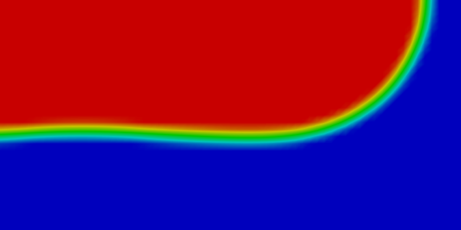
Results for minimizing the mean compliance of a cantilever beam for three different phase field parameters are shown in Figure 2. Here we chose the weighting factor for the Ginzburg Landau energy . Already for one obtains the same structure as for the smallest value of the phase field parameter, i.e. the right qualitative behaviour of the sharp interface minimizer. We also remark that for the smallest value of , the interface is already very thin and almost not visible anymore.
We want to study the convergence of the minimizers . For this purpose we denote by a minimizer for the sharp interface problem. As this minimizer is a priori unknown, we approximate by , where . Thus the optimal interface is approximated by the zero level set of , denoted by . The difference can be separated into two terms,
| (35) |
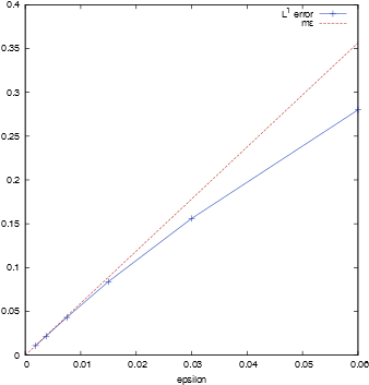
where denotes the constructed recovery sequence corresponding to and exposes a -profile normal to , see [15]. We want to determine which term of the error in is the dominating part. We notice that the first term on the right-hand side of can be considered as the distance of the zero level sets of and and the second term describes the error resulting from the diffuse interface profile. The 1D error of the -profile compared to a characteristic function is given by . Thus, the -error in our setting can be approximated by . As the perimeter is not known, we extrapolate the given sequence numerically to , which gives . As mentioned above, from the -convergence result of [15, 33] it is expected that . Hence, we may approximate with .
In Figure 3(a) we depict now the difference (solid blue line) together with the approximated diffuse interface error (dashed red line). We see that for the -difference of the minimizer and the approximated minimizer becomes tangential to the line . This indicates that the error resulting from the diffuse interface profile dominates the total approximated error in and that the distance of the zero level sets becomes comparably small. Hence, the level set of is already for a good approximation of the optimal interface .
To complete this picture we also give a plot of the minimal functional values and the Lagrange multipliers for the calculated values in Figure 3(b) and 3(c). One sees that is monotonically decreasing as decreases and seems to converge linearly to a specific value, supposedly a minimal value for , compare also Theorem 20. Likewise, converges linearly to a limit value , compare Theorem 21.
To study the influence of the perimeter penalization, we carried out the same calculations for a smaller weighting factor . We can control the appearance of fine structures by the choice of . As an example, we refer to Figure 1(b), where we used the parameters , . This verifies numerically that the regularization yields a well-posed problem but still gives desired optimal structures. Moreover, the influence of regularization parameters on the fineness of the structure is in accordance to other methods (see e.g. [8]). For the computation we chose the inner product
which depends on the current iterate and which includes second order information of the Ginzburg-Landau energy, as well as of the compliance part. Here, we used and which is given as the solution of the linearized state equation
3.3 Optimal material distribution within a wing
We now consider a different geometry for the overall container in a three dimensional setting. This example shows that we can also use different geometries, i.e. different choices of , and work in a three dimensional setting.
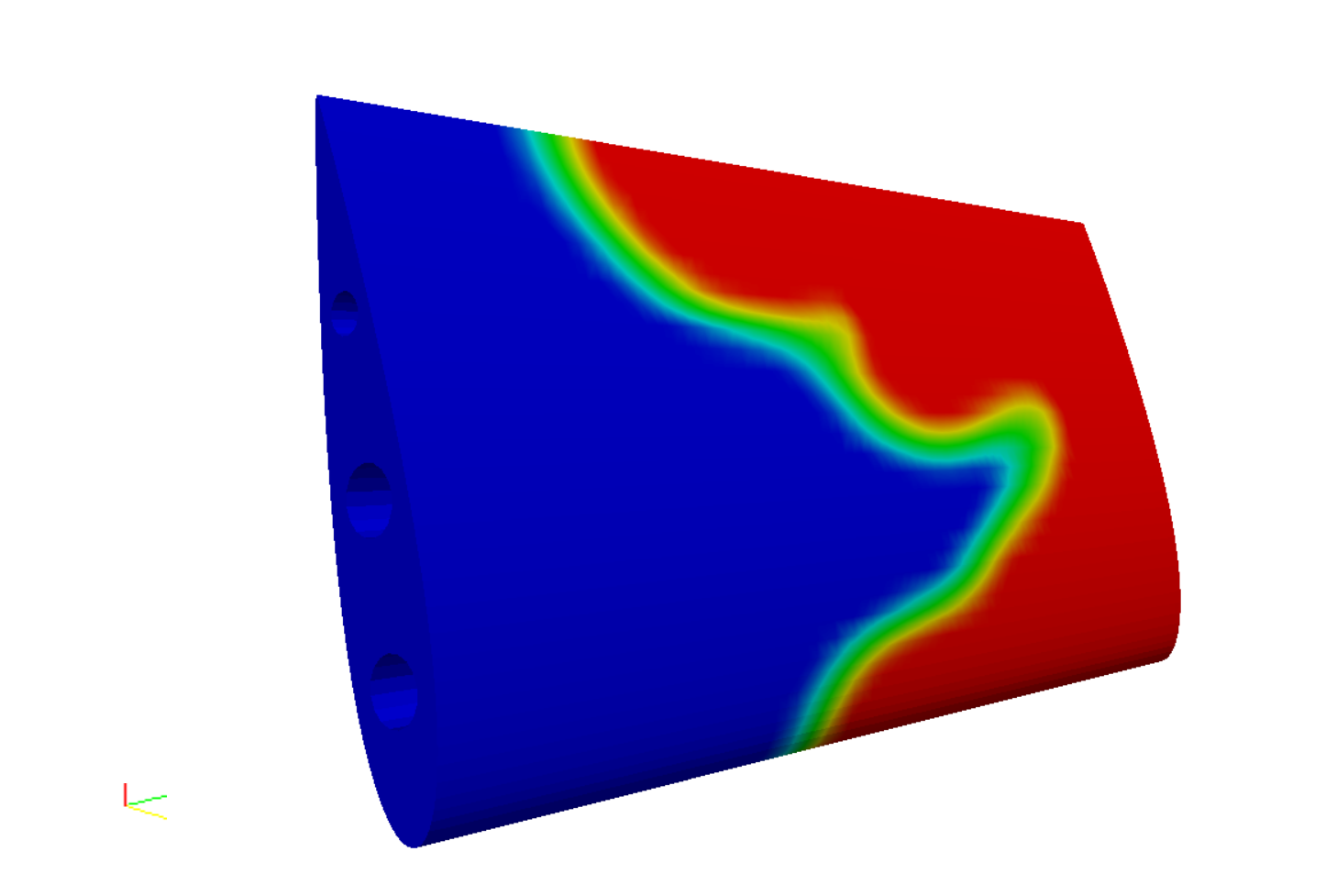
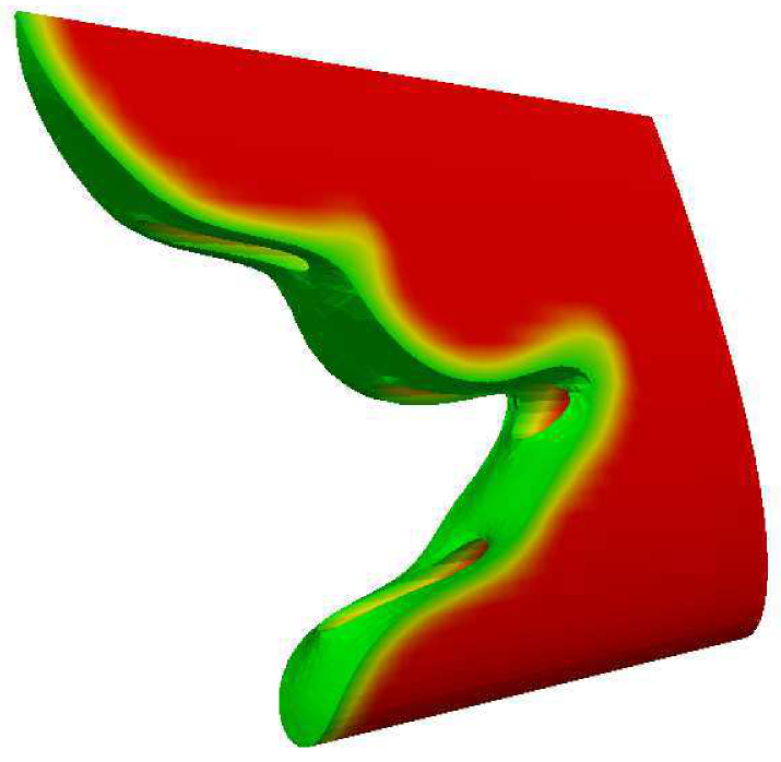
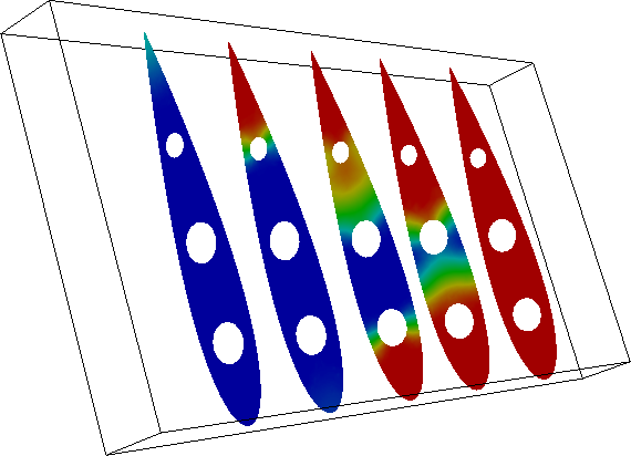
We perform the same optimization strategy as above and optimize the material configuration within a wing of an airplane. This example is to be considered as an outlook on possible applications. One wants to have a composite material in order to obtain a high ratio of stiffness to weight. Hence we use one very stiff material () and a material representing the light material (, ). As geometry we use a three dimensional NACA 0018 airfoil configuration with three holes in it. The configuration can be seen in Figure 4.
The considerations of the previous example have shown that we do not have to choose too small in order to obtain the right qualitative behaviour and so we use here . Moreover, the weighting factor for the Ginzburg-Landau regularization is chosen quite small, i.e. . The boundary force is of elliptic form, which is typical for the lift force acting on an airplane wing, compare for instance [23]. Its support is on . The Dirichlet boundary is the part where the wing is attached to the airplane (left-hand side in Figure 4). The optimized material configuration is shown in Figure 4, where the blue material is the stiff material. We also give a picture of the weak material, i.e. the set , see Figure 4, in order to see the hypersurface separating the two materials, together with various cross sections of the wing.
3.4 Influence of eigenstrain
4 Derivation of the optimality conditions
In this section we will give the proofs of Theorem 12 and Theorem 17. We start with showing the differentiability of at for and , and deriving the validity of :
Lemma 23.
Proof.
The idea is to apply the implicit function theorem and hence we define for small enough the function by
Using the calculation rules , for we can establish
where we made use of if by the particular choice of . Besides, , given by
is by Lax-Milgram’s theorem an isomorphism. And so we can apply the implicit function theorem to obtain differentiability of at together with , and obtain therefrom . ∎
Now we can directly proof the validity of the optimality system for the sharp interface problem:
Proof of Theorem 12: The formula for the first variation of the perimeter functional can for instance be found in [29, 10.2]. The volume integrals appearing in the objective functional can be differentiated directly by using change of variables. To handle the boundary integrals, we use the calculation rules derived in [21, Chapter 9, Section 4.2] to see
where , . The derivative of with respect to at can be calculated by For more details we refer to [21]. And so we arrive in
where is already determined by Lemma 23.
The existence of a Lagrange multiplier for the integral constraint follows as in [30, Lemma 7.5], see also [28]. For the sake of readability, we restate here the main steps of this proof. First we may assume without loss of generality that , otherwise any transformation will yield admissible comparison functions for and in this case is the desired Lagrange multiplier. Considering the case , we choose some with associated transformation such that and define by for small enough. Direct calculation yields . And so we apply the implicit function theorem to obtain such that for , . Hence for and thus . One can then establish that
where we defined . As we chose we have that , hence , for . This shows and yields in particular that is a Lagrange multiplier.
Similarly, we directly establish the corresponding optimality system for the phase field problems:
5 Proof of the convergence results
In this section we want to prove the convergence results stated in Theorem 19 and Theorem 21. First, we want to give a proof of the -convergence result of Theorem 19. For this purpose, we start with the following lemma:
Lemma 24.
Proof.
Let be a sequence such that a.e. in for every and . In particular, this gives directly a.e. in . Now let be any subsequence of . Defining we see that it holds
Thus, by applying the inequalities of Korn, Young and Hölder and the uniform estimate on the elasticity tensor , see , we obtain that
And so we find a subsequence such that converges weakly in to some as . Using the uniform boundedness of the tensor-valued function , see Assumption (A3), we obtain for any the uniform estimate
Hence, Lebesgue’s convergence theorem implies that converges strongly in to . Since converges additionally weakly in , we obtain that
Similarly, we can deduce from the uniform boundedness of that
This leads to
which yields . By applying the same arguments as above for any subsequence of , we obtain that every subsequence of has a subsequence such that converges weakly in to . This implies then the demicontinuity of as stated in the lemma.
We are left with proving the continuity of . For this purpose, we take again a sequence such that a.e. in and . We have already established, that this implies the weak convergence of to in . Using the compact imbeddings and we moreover find, that converges strongly in and converges strongly in . We can now use the continuity of the objective functional stated in Assumption (A5), see Remark 3, to obtain and have shown the statement. ∎
Using this lemma, we can show Theorem 19 by applying known results concerning -convergence of the Ginzburg-Landau energy.
Proof of Theorem 19: By [33] we obtain, that the Ginzburg-Landau energy , which is given by
-converges as in to
We rewrite the reduced objective functional in the following form: , where if and if with
Making use of Lemma 24, we find that is a continuous function in , and so is the Ginzburg-Landau energy plus some functional which is continuous in . Consequently, by standard results for -convergence, see for instance [19], we find that -converges in to , since This proves the statement.
Now we want to prove the convergence of the equations of the first variation:
Proof of Theorem 21:
The result of Corollary 20 yields directly the existence of a subsequence of converging in to a minimizer of such that . By Lemma 24, this implies the weak convergence of to in as .
Now we recall, that is given as the solution of
| (36) |
where is given by
Since is uniformly bounded in , and using the uniform estimate on the elasticity tensor and the eigenstrain given by Assumptions (A3) and (A4) we can deduce that And so we find by Korn’s inequality from that This yields the existence of a subsequence, which will be denoted by the same, such that converges weakly in to . Following the arguments of the proof of Lemma 24 we see that the limit element of fulfills . Hence, by definition of , see Theorem 12, we get . In particular, we can deduce by the imbedding theorems that both and converge strongly in and . And so we obtain by the continuous differentiability of the objective functional, see Remark 4, that
| (37) |
Analogously as in [28] we can apply the Reshetnyak continuity theorem to deduce
| (38) |
Plugging those results together we end up with . As in [28] we can find some such that if we assume . Thus we have
wherefrom we obtain that converges to some . Besides, this directly yields that fulfills and thus is a Lagrange multiplier associated to the integral constraint. This finally proves the statement.
6 Conclusions
We have shown that the proposed phase field approach leads to an optimal control problem for which existence of a solution can be shown. The problem can be reformulated in such a way that a reduced objective functional has to be minimized. The latter -converges in as the thickness of the interface tends to zero to a functional describing a sharp interface formulation of the problem. We have shown that certain first order optimality conditions for the phase field problem can be deduced by geometric variations. As the minimizers converge, also the obtained optimality conditions converge to a system, which is a necessary optimality condition for the sharp interface problem. Besides, this optimality system for the sharp interface problem can be derived in the general setting of functions of bounded variations.
Assuming additional regularity assumptions on the minimizing set and the data, it can be shown that the obtained conditions are equivalent to results that were already obtained in literature by classical shape calculus and also by formal asymptotics from the phase field model. Thus we have delivered a rigorous proof for the convergence results that were already predicted by formal asymptotics in [11]. Moreover we use a general objective functional. However, in [11] the state constraints can be -dependent. To be precise, an ersatz material approach is used, where the stiffness of the ersatz material scales like , and thus vanishes as . This is not done in our work, but possible generalizations for reasonable objective functionals in the spirit of [27, 28] may be possible. This means that convergence of minimizers could possibly be shown, but we expect that again certain growth conditions on the convergence of the minimizers play a role, where this rate has to be consistent with the -scaling of the ersatz material.
We presented numerical simulations which were obtained with the help of a projected gradient type method which showed that the proposed phase field approach works well in two and three spatial dimensions.
References
- [1] G. Allaire, C. Dapogny, G. Delgado, and G. Michailidis, Multi-phase structural optimization via a level set method, COCV, 20 (2014), pp. 576–611.
- [2] G. Allaire and F. Jouve, A level-set method for vibration and multiple loads structural optimization, Comput. Methods Appl. Mech. Engrg., 194 (2005), pp. 3269–3290.
- [3] G. Allaire, F. Jouve, and A.-M. Toader, Structural optimization using sensitivity analysis and a level-set method, Journal of Computational Physics, 194 (2004), pp. 363 – 393.
- [4] G. Allaire, F. Jouve, and N. Van Goethem, Damage evolution in brittle materials by shape and topological sensitivity analysis, J. Comput. Phys., 230 (2011), pp. 5010–5044.
- [5] L. Ambrosio and G. Buttazzo, An optimal design problem with perimeter penalization, Calc. Var. Partial Differential Equations, 1 (1993), pp. 55–69.
- [6] L. Ambrosio, N. Fusco, and D. Pallara, Functions of Bounded Variation and Free Discontinuity Problems, Oxford: Clarendon Press, 2000.
- [7] J. Barrett, R. Nürnberg, and V. Styles, Finite Element Approximation of a Phase Field Model for Void Electromigration, SIAM J. Numer. Anal., 42 (2004), pp. 738–772.
- [8] M. Bendsøe, Topology optimization: theory, methods and applications, Springer, 2003.
- [9] M. Bendsøe, R. Haber, and C. Jog, A new approach to variable-topology shape design using a constraint on perimeter, Struct. Multidiscip. Optim., 11 (1996), pp. 1–12.
- [10] M. Bergounioux, K. Ito, and K. Kunisch, Primal-dual strategy for constrained optimal control problems, SIAM Journal on Control and Optimization, 37 (1999), pp. 1176–1194.
- [11] L. Blank, H. Farshbaf-Shaker, H. Garcke, and V. Styles, Relating phase field and sharp interface approaches to structural topology optimization, ESAIM: COCV, 20 (2014), pp. 1024–1058.
- [12] L. Blank, M. Farshbaf-Shaker, H. Garcke, C. Rupprecht, and V. Styles, Multi-material phase field approach to structural topology optimization, in Trends in PDE Constrained Optimization, G. Leugering, P. Benner, S. Engell, A. Griewank, H. Harbrecht, M. Hinze, R. Rannacher, and S. Ulbrich, eds., ISNM, Birkhäuser, to appear.
- [13] L. Blank, H. Garcke, L. Sarbu, T. Srisupattarawanit, V. Styles, and A. Voigt, Phase-field approaches to structural topology optimization, in Constrained Optimization and Optimal Control for Partial Differential Equations, G. Leugering, S. Engell, M. Hinze, R. Rannacher, V. Schulz, V. Ulbrich, and S. Ulbrich, eds., vol. 160 of ISNM, Birkhäuser, 2012, pp. 245–256.
- [14] L. Blank and C. Rupprecht, An extension of the projected gradient method to a Banach space setting with application in structural topology optimization. arXiv:1503.03783v2.
- [15] J. F. Blowey and C. M. Elliott, The Cahn-Hilliard gradient theory for phase separation with non-smooth free energy Part I: Mathematical analysis, European J. Appl. Math., 2 (1991), pp. 233–280.
- [16] B. Bourdin and A. Chambolle, Design-dependent loads in topology optimization, ESAIM Control Optim. Calc. Var., 9 (2003), pp. 19–48.
- [17] D. Braess, Finite Elemente, Springer, 1997.
- [18] P. Ciarlet, Three-Dimensional Elasticity, vol. 1 of Studies in mathematics and its applications, Elsevier Science, 1988.
- [19] G. Dal Maso, An Introduction to -convergence, Progress in Nonlinear Differential Equations and Their Applications, Birkhäuser, 1993.
- [20] M. Delfour and J. Zolésio, Shapes and Geometries: Analysis, Differential Calculus, and Optimization, Adv. Des. Control, SIAM, 2001.
- [21] , Shapes and Geometries: Metrics, Analysis, Differential Calculus and Optimization, Adv. Des. Control, SIAM, 2011.
- [22] M. Delfour and J. Zolésio, Shape derivatives for nonsmooth domains, in Optimal Control of Partial Differential Equations, K.-H. Hoffmann and W. Krabs, eds., vol. 149 of Lecture Notes in Control and Inform. Sci., Springer, 1991, pp. 38–55.
- [23] C. Dorand, Influence of Elliptical Distribution of Lift on Strength of Airplane Wings, Technical memorandum, National Advisory Committee for Aeronautics, 1922.
- [24] C. Eck, H. Garcke, and P. Knabner, Mathematische Modellierung, Springer, 2008.
- [25] L. Evans and R. Gariepy, Measure Theory and Fine Properties of Functions, Mathematical Chemistry Series, CRC PressINC, 1992.
- [26] H. Garcke, The -limit of the Ginzburg-Landau energy in an elastic medium, AMSA, 18 (2008), pp. 345–379.
- [27] H. Garcke and C. Hecht, A phase field approach for shape and topology optimization in Stokes flow, Preprint-Nr.: 09/2014, Universität Regensburg, Mathematik, (2014).
- [28] , Shape and topology optimization in Stokes flow with a phase field approach, Preprint-Nr.: 10/2014, Universität Regensburg, Mathematik, (2014).
- [29] E. Giusti, Minimal surfaces and functions of bounded variation, Notes on pure mathematics, Dept. of Pure Mathematics, 1977.
- [30] C. Hecht, Shape and topology optimization in fluids using a phase field approach and an application in structural optimization, Dissertation, University of Regensburg, 2014.
- [31] M. Hintermüller, D. Hömberg, and K. Sturm, Shape optimization for a sharp interface model of distortion compensation. WIAS Preprint No. 1792, 2013.
- [32] A. G. M. Michell, The limits of economy of material in frame-structures, Phil. Mag., 8 (1904), pp. 589–597.
- [33] L. Modica, The gradient theory of phase transitions and the minimal interface criterion, Arch. Ration. Mech. Anal., 98 (1987), pp. 123–142.
- [34] L. Modica and S. Mortola, Un esempio di -convergenza, Boll. Un. Mat. Ital. B (5), 14 (1977), pp. 285–299.
- [35] D. Sale, A. Aliseda, M. Motley, and Y. Li, Structural Optimization of Composite Blades for Wind and Hydrokinetic Turbines, Proceedings of the 1st Marine Energy Technology Symposium METS 2013, (2013).
- [36] R. Showalter, Monotone Operators in Banach Spaces and Nonlinear Partial Differential Equations, Mathematical surveys and monographs, v. 49, American Mathematical Society, 1997.
- [37] J. Thomsen, Topology optimization of structures composed of one or two materials, Structural optimization, 5 (1992), pp. 108–115.