Andrew Wiles Building, Woodstock Road
Oxford OX2 6GG, UK bbinstitutetext: Department of Physics and Astronomy,Uppsala University
SE-751 20 Uppsala, Swedenccinstitutetext: Sorbonne Universités, UPMC Univ. Paris 06, UMR 7589, LPTHE, F-75005, Paris, Franceddinstitutetext: CNRS, UMR 7589, LPTHE, F-75005, Paris, Franceeeinstitutetext: Sorbonne Universités, Institut Lagrange de Paris, 98 bis Bd Arago, 75014 Paris, France
Exploring Structure Moduli Spaces with Integrable Structures
Abstract
We study the moduli space of structure manifolds that form the internal compact spaces in four-dimensional domain wall solutions of heterotic supergravity with flux. Together with the direction perpendicular to the four-dimensional domain wall, forms a non-compact 7-manifold with torsionful structure. We use this embedding to explore how varies along paths in the structure moduli space. Our analysis includes the Bianchi identities which strongly constrain the flow. We show that requiring that the structure torsion is preserved along the path leads to constraints on the torsion and the embedding of in . Furthermore, we study flows along which the torsion classes of go from zero to non-zero values. In particular, we present evidence that the flow of half-flat structures may contain Calabi–Yau loci, in the presence of non-vanishing -flux.
1 Introduction
Compactifications of string theory provide one of the most fruitful grounds for the study of the theory’s formal and phenomenological aspects. String compactifications can also be used as a tool to study properties of compact manifolds, and has been instrumental in the study of Calabi–Yau manifolds. In particular, the demand that supersymmetry is preserved leads to severe constraints on the metric of the compactified space. In heterotic string theory, the conditions for supersymmetric, maximally symmetric, four-dimensional vacua have long been known: with vanishing flux , the internal 6-manifold must be Calabi–Yau Candelas:1985en , whereas a non-zero -flux requires the internal geometry to be complex non-Kähler Strominger:1986uh ; Hull:1986kz (see Lust:1986ix ; Dasgupta:1999ss ; Ivanov:2000fg ; Becker:2002sx ; Becker:2003sh ; Becker:2003yv ; Gauntlett:2002sc ; Cardoso:2002hd ; Gauntlett:2003cy ; Gran:2005wf ; Becker:2006xp ; Gran:2007kh ; Ivanov:2009rh for further discussions). These two types of 6-manifolds both allow a globally defined, nowhere vanishing spinor , that can be used to decompose the ten-dimensional supercharge of heterotic supergravity into internal and external components, . If the external spinor component is covariantly constant, it provides a four-dimensional supercharge and guarantees that the four-dimensional vacuum has supersymmetry.
All six-dimensional manifolds with one nowhere vanishing spinor have structure, and so their geometry is completely specified by a real two-form and a complex three-form that need not be closed Hitchin:2000jd ; chiossi . The non-closure of and determines the intrinsic torsion of the geometry. In this language, Calabi–Yau manifolds correspond to torsion-free structures, and the spaces that are solutions to the Strominger system Strominger:1986uh ; Hull:1986kz have torsion components transforming in a particular irreducible representation Cardoso:2002hd ; Gauntlett:2003cy .111 structure manifolds are also relevant for (supersymmetric) type II compactifications with flux, and reviews of this topic can be found in Grana:2005jc ; Blumenhagen:2006ci ; Koerber:2010bx . A summary of the torsion constraints that also includes non-supersymmetric vacua can be found in section 2 of Larfors:2013zva .
If the restrictions on the torsion of the internal structure manifold are relaxed, the resulting vacuum will break supersymmetry. More general structure manifolds can thus provide interesting non-supersymmetric vacua of heterotic string theory, with the benefit that the structure guarantees an four-dimensional effective field theory description of the low-energy dynamics. A simple class of such vacua, that will be studied in this paper, are half-BPS domain wall solutions in four dimensions, that preserve supersymmetry. As has been shown recently Gray:2012md , the supersymmetry constraints put very mild restrictions on the intrinsic torsion; for the most general -flux preserving the symmetry of the ansatz, almost all torsion components can be balanced by the appropriate flux (for studies with restricted flux, see Lukas:2010mf ; Klaput:2011mz ; Klaput:2012vv ; Klaput:2013nla for a ten-dimensional perspective, and Gurrieri:2004dt ; Micu:2004tz ; deCarlos:2005kh ; Gurrieri:2007jg ; Micu:2009ci for four-dimensional studies). This heterotic set-up can thus be used to study the properties of many different types of structure manifolds.
The scope of this paper is to use heterotic domain wall solutions to explore the moduli space of different structure manifolds. We restrict our study to the zeroth order approximation of heterotic string theory,222The heterotic gauge fields appear at first order in , and are neglected in our study, as are the corrections to the Bianchi identity of . Note however that domain wall solutions avoid the usual no-go theorems for -flux that appear at zeroth order in solutions Ivanov:2000fg ; Gauntlett:2003cy , since the compactification is on a seven-dimensional non-compact manifold. so that the bosonic part of the ten-dimensional supergravity action reduces to
| (1) |
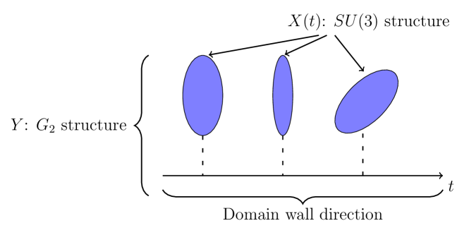
where is the ten-dimensional metric, the corresponding Ricci scalar, the dilaton, and the flux of the Kalb–Ramond field , satisfying the Bianchi identity . We look for solutions where spacetime decomposes into a warped product of a compact structure manifold and a four-dimensional non-compact spacetime. The latter decomposes, for domain wall solutions, into a maximally symmetric three-dimensional space along the domain wall world-volume and a direction perpendicular to the wall. Alternatively, as depicted in figure 1, we may combine the direction perpendicular to the domain wall with the structure manifold to a non-compact seven-dimensional manifold with structure Lukas:2010mf ; Gray:2012md . The spacetime metric thus has the form
| (2) |
where the function and structure metric depend both on and the coordinates on . For the -flux, we allow all components that preserve the symmetries of the metric; along the maximally symmetric three-dimensional spacetime, and along the seven-dimensional manifold.
The supersymmetry constraints and the Bianchi identity for can, as we show in section 2, be reformulated as constraints on the intrinsic torsion of the structure. For the most general flux compatible with the spacetime symmetries, these conditions are met by a certain type of integrable structures. Consequently, the physical problem of finding supersymmetric domain wall solutions in heterotic string theory translates into the mathematical problem of determining how the structure, dilaton and flux flow to form an integrable structure. The solutions are thus generalisations of Hitchin flow Hitchin:2000jd , where a half-flat structure manifold varies over a perpendicular direction to form a seven-manifold with holonomy. Indeed, the Hitchin flow is reproduced by the domain wall solutions when the flux is set to zero, and the dilaton is taken to be constant. Other types of flows have been discussed by Chiossi and Salamon chiossi .
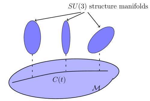
As the structure flow along the domain wall direction, it will trace out a curve in the moduli space of structure manifolds, see figure 2. Consequently, through these constructions we uncover information about the parameter space of generic structure manifolds, which is highly non-trivial to study. For Calabi–Yau metrics, the parameters decompose into moduli corresponding to variations of the closed forms and : the former describe variations of the Kähler structure, and the latter variations of the complex structure, and the dimension of the two spaces is determined by the Hodge numbers and of the Calabi–Yau three-fold, respectively Candelas:1990pi . On generic structure manifolds, neither nor are closed, and the relevant parameters are only partially known (see Tseng:2009gr ; Tseng:2010kt ; Tseng:2011gv for some recent progress). Indeed, care is needed when studying the moduli, since even very basic questions, such as the dimensionality of the parameter space, become subtle. As an example, the moduli space of deformations of in the Strominger system appears infinite-dimensional Becker:2006xp , unless deformations of the -corrected Bianchi identity for are simultaneously taken into account Anderson:2014xha ; delaOssa:2014cia .
In the present paper, the embedding constrains the allowed deformations, and thus simplifies the variational analysis. While this restriction means that questions regarding the number of parameters cannot be addressed, the setting is rich enough to tackle non-trivial questions such as the connections between the moduli spaces of Calabi–Yau and non-Calabi–Yau manifolds. With the most general -flux, the heterotic constraints are solved by a wide range of structure manifolds, and different domain wall solutions may connect structures of different type. Through these constructions, we can thus study whether certain properties, such as an integrable complex structure, are preserved or violated by the flow, and whether torsion classes or flux components can be switched on and off by the flow. As a result, we will gain insight about the interconnections between the parameter spaces of different structure manifolds.
The rest of this paper is organised as follows. We start, in section 2, by presenting the integrable structures that are relevant for domain wall solutions. We translate the supersymmetry conditions and Bianchi identities, which imply the equations of motion for the supergravity fields, into constraints on the torsion classes. In section 3, we analyse the same equations from the perspective of the structure manifolds. We derive the constraints on the variations of the structure forms, and find that the flow of is completely determined by the torsion and flux, whereas some freedom remain in the variation of . In the following sections, we give examples of different types of structure flows that illustrate the intricacy of the moduli space of such manifolds. In section 4, we study the flow of Calabi–Yau manifolds with flux: we derive the constraints on the flow to preserve the Calabi–Yau properties, and perform a first-order analysis of the flow without these constraints that show that non-zero torsion is induced. In sections 5 and 6, we study the flow of nearly Kähler and half-flat structures. We determine the constraints required to preserve the torsion along the flow, and study whether loci with vanishing torsion are possible. In section 7 we summarise our results and discuss possible extensions of our analysis. Our conventions are summarised in appendix A. In a separate paper OKS , a complementary study of the embedding of the Strominger system into and Spin(7) manifolds will be presented.
2 domain wall solution and structures
In this paper, we are interested in four-dimensional domain wall solutions of heterotic string theory that preserve supersymmetry. Such configurations arise from heterotic compactifications on six-dimensional manifolds with structure. Alternatively, as shown in Figure 1, they can be viewed as three-dimensional maximally symmetric heterotic solutions that result from “compactification” on a non-compact seven-dimensional structure manifold , that is foliated by the six-manifolds. In this section, we describe how supersymmetry determines the structure of .
Any heterotic vacuum solution must satisfy the equations of motion and Bianchi identities of the low-energy supergravity description of the theory. For supersymmetric solutions, the vanishing of the supersymmetry variations of fermionic fields lead to additional constraints. As described in detail in Lukas:2010mf ; Gray:2012md , to lowest order in the expansion, these constraints require the existence of a three-form on , that must satisfy the following constraints
| (3) | ||||
| (4) | ||||
| (5) | ||||
| (6) |
where the three-form and the function are the components of the ten-dimensional flux , which lie along and the three-dimensional, maximally symmetric domain wall world-volume, respectively.333The flux component determines the cosmological constant of the three-dimensional spacetime; a non-zero gives a anti de Sitter spacetime, while a vanishing gives Minkowsi spacetime. is the ten-dimensional dilaton, and is the seven-dimensional Hodge dual of . and denote the exterior derivative and Hodge dual on , respectively (see appendix A for further conventions).
This system is equivalent to a structure FerGray82 ; chiossi determined by
| (7) | ||||
| (8) |
with intrinsic torsion specified by
| (9) | ||||
| (10) | ||||
| (11) | ||||
| (12) |
The torsion classes , are -forms that transform in irreducible representations of . The torsion class must satisfy the primitivity constraints
and the stucture is called integrable when , as is the case here. In the above equations, we have decomposed into components that are parallel and orthogonal to :
By further restricting the flux, the torsion class can be set to zero so that the structure is integrable conformally balanced Firedrich:2003 ; this case is studied in Gauntlett:2002sc ; Gran:2005wf ; Lukas:2010mf .
It is straight-forward to prove the equivalence between (3)-(6) and (7)-(12). The equations for and are obvious, whereas the remaining equations require some work. Comparing equations (7) and (3) we obtain
| (13) |
Using the first primitivity constraint on in (13) gives the relation
Decomposing as , with as above, we have , and thus
Using this in equation (13), and taking the Hodge-dual, we find
The second primitivity constraint on now gives
It turns out that this equation is equivalent to (5). In fact,
The last equation (6) gives
and therefore
This concludes the proof of the equivalence between (3)-(6) and (7)-(12). For future reference, we record the inverse relations for , and in terms of the torsion classes
| (14) |
In addition to the supersymmetry equations, heterotic vacuum solutions have to satisfy the equations of motion and the Bianchi identities. At lowest order in , the latter is
Inserting (14) in these relations, we find further constraints on the torsion:
| (15) |
Finally, we turn to the equations of motion. At lowest order in , the former comprise Einstein’s equations, the equation of motion for the dilaton and the equations of motion for the flux . To first order in the expansion, it has been shown Gauntlett:2002sc ; Ivanov:2009rh that both Einstein’s equations and the equation of motion for the dilaton are implied by the supersymmetry equations, Bianchi identity and flux equations of motion, and so provide no further constraint on the structure. An extension of this result, that includes the flux equation of motion in the equations implied by supersymmetry and the Bianchi identities, can be found in Martelli:2010jx . Let us provide an alternative proof for this last point. The seven-dimensional flux equation of motion are
| (16) | ||||
This equation is also implied by the Killing spinor equations and Bianchi identities, as we now show. Clearly, the supersymmetry constraints and the Bianchi identities set the first three terms on the right hand side of the second equation in (16) to zero. What remains is
| (17) |
This should be compared to
| (18) |
where the last bracket vanish as a consequence of the supersymmetry conditions and Bianchi identities. Thus, to zeroth order in , all equations of motion follow from the Killing spinor equations and Bianchi identities, and the structure is completely specified by (7)-(12) in conjunction with the differential constraints (15).
3 structures embedded into integrable structures
In this section, we derive the constraints that the Killing spinor equations and Bianchi identities of domain wall solutions put on the structure of . Mathematically, these constraints determine how the structure embeds into integrable structures. As in the previous section, we start with the supersymmetry constraints, and then proceed to the Bianchi identities.
3.1 The embedding
Consider a manifold with an structure Gray:1980fk ; chiossi ; Cardoso:2002hd ; Gauntlett:2003cy determined by the complex -form and the real form which satisfy the compatibility equations
| (19) |
and the torsion structure equations
| (20) | ||||
| (21) |
where is a complex function, is a primitive -form, is a real primitive 3-form of type , and and are 1-forms. The torsion components and are the Lee-forms of and respectively.
The structure forms determine both the almost complex structure (determined by the real part of ), and the metric on the manifold Hitchin01stableforms , see appendix A. The torsion classes are related to the Nijenhuis tensor of the almost complex structure, and vanish if and only if the latter is integrable.
We now embed the structure into an integrable structure , by choosing a 1-form and a complex valued function such that
| (22) |
The Hodge dual of is
| (23) |
where we have used
and the metric on induced by the structure which is
| (24) |
Note that we are not assuming that the metric on is independent of . The structure varies with and so does the metric on . As and the metric on are covariantly constant (with respect to the connection with torsion), is a constant on , , and therefore so is
It is important however to keep in mind that all these quantities may depend on . Note also that different choices of correspond to same almost complex structure on , however they give different embeddings of the structure into the structure.
Recall that an integrable structure satisfies . Thus the torsion structure equations for are
| (25) | ||||
| (26) |
The torsion class belongs to , that is
| (27) |
The torsion class is therefore
| (28) |
For these structures the 1-form is not in general closed. Since we are interested in the domain wall solutions of Section 2, we restrict the structure so that is exact
To embed the structure into an integrable structure, we need to decompose the torsion classes as follows
| (29) | ||||
| (30) |
where
The constraints on , equations (27), can be decomposed using equation (30). The first constraint gives
| (31) |
and the second
| (32) |
The following identities will be useful in our computations.
Lemma 1.
Let
Then
where is the argument of .
Proof.
To embed the structure into an integrable structure, we use equations (22) and (23), into the equations (25) and (26).
Proposition 1.
The embedding given by equations (22) and (23) of the structure with torsion classes as in (20) and (21) into an integrable structure with torsion classes (25) and(26) gives the the following relations between the torsion classes and the flow of and with respect to the coordinate :
| (33) | ||||
| (34) | ||||
| (35) | ||||
| (36) | ||||
| (37) | ||||
| (38) | ||||
Proof.
We begin our analysis of the embedding with equation (26) (which enforces the condition that ). Using equations (22) and (23) and Lemma 1, we obtain
which gives equations (33) and (34)
The last of these equations gives the first identity in (34) and we obtain the second after using Lemma 1. Equations (35) can be obtained from equation (34) using the formula
and recalling that for any -form
Now we turn to equation (25). Equation (36) can be easily obtained by computing using equations (28) and (25):
Taking the Hodge dual, we obtain equation (36) where we have used
Using equations (22) and (23) into equation (25) we obtain
from which we find two relations
The first one gives a relation between the torsion classes of the structure and the structure which we can write, for example, as an equation for . Using Lemma 1 we find
| (39) | ||||
Taking the Hodge dual, we find equation (37). This relation is a flow equation for which, using Lemma 1, gives equation (38). ∎
It will be useful for later to have an expression for which satisfies the contraints in equations (31) and (32).
Proposition 2.
| (40) |
where is a primitive 3-form of type .
Proof.
We begin by writing the Lefshetz decomposition of
Also, the Hodge decomposition of can be written as
where is of type . Using equation (39) into the second equation in (32) we obtain
which gives the first term in equation (40). The first relation in equation (32) gives
whereas the Hodge dual of equation (31) gives
Putting all this together we obtain equation (40). By computing the Hodge dual of (40), we obtain an equation for . ∎
3.2 Flow equations and moduli
The manifold is an almost-hermitian manifold with an structure. Its almost-complex structure is completely determined by , and therefore, the flow of corresponds to variations of the almost complex structure of as varies. On the other hand, the flow of has simultaneous variations of both the hermitian structure and those of the almost complex structure.
The variations of can be written as
| (42) |
where is a function on and is a primitive real 2-form on . Comparing the flow equation for (35) with (42) we have
where we have defined the form
| (43) |
for later convenience. It is very interesting to note that vanishes for all structures for which vanishes. In these cases the structure deforms with such that the hermitian structure is fixed.
The variations of with respect to are given by MR0112154 ; 0128.16902
| (44) |
where is a complex valued function on and is a -form on . As , we also have
The variation of the volume form compatibility condition (19) of structure gives
is constant on up to diffeomorphisms, and therefore is constant on . Both functions can vary with
Therefore
where we have used equation (24). Comparing with the flow equation (41) we find
| (45) | ||||
| (46) |
We can obtain by taking the component of the equation for :
| (47) |
As , the structure equation for
becomes
This needs to be compatible with the flow equation (34) for which can now be written as
Therefore, the 4-form , flows into another -closed 4-form in the same cohomology class as . Consider now the equations for . The flow equation (35) can be written as
This expression must be a solution to the variation of the integrability equation (20)
| (48) |
Plugging into this equation the expression for above, gives a non-trial equation for the variation of the torsion class
| (49) |
3.3 Bianchi identities
The supersymmetric solutions we have discussed need to satisfy the Bianchi identities. We consider these identities as a further constraint on the integrable structure . Recall
The Bianchi identities state that is closed
and that is a constant on . We express these constraints as constraints on the structure embedded into the structure.
Let
Then
where
and we have used
Now the Bianchi identity gives
from which we obtain two equations
| (51) | ||||
This means that variations of a solution in a cohomology class in remain in the same cohomology class.
3.4 Summary of constraints
Since this is a long section, let us briefly recall the constraints that supersymmetry and the Bianchi identities put on the the structure.
-
•
The Lie form is exact: .
-
•
The embedding of the structure into an integrable structure is specified through (22) by a real function and a complex function .
-
•
The remaining torsion classes , and can take on different values, and determine, together with and , the NS flux components and , as well as the flow of and .
-
•
The Bianchi identities (51) further constrain the structure.
In addition, the flow of the structure is determined by
| (52) |
4 Example: Flow of Calabi–Yau manifold with flux
In this, and the two following sections, we will determine the flow of structure manifolds with restricted torsion. The aim is to study how the constraints from the embedding structure determines a path in the moduli space of the structure manifolds. We will show that flows can be structure-preserving, so that a fixed set of torsion classes are non-zero along the flow. Flows where the torsion classes change are also allowed, and will be analysed from different perspectives.
To simplify our calculations, we henceforth work in the gauge . This means in particular that we have absorbed the phase in . As a consequence, the phases of change, and is modified by . Moreover, in the gauge we have for all values of . In this case we have the relation
| (53) |
The simplest structure is when all torsion classes are zero so that the manifold is Calabi–Yau. We now determine the necessary and sufficient constraints on the flow so that the three-fold stays Calabi–Yau to all orders in . In the next subsection, we will compute the torsion classes generated at linear order in , once these constraints fail to hold. A summary and discussion of the result from this perturbative analysis is found in the last subsection.
4.1 Calabi–Yau to all orders
Proposition 3.
The domain wall flow preserves the Calabi–Yau conditions if and only if and is harmonic.
Proof.
Suppose that all torsion classes vanish. Then the general analysis gives
| (54) | ||||
| (55) | ||||
| (56) |
Note that is -constant whenever the form is holomorphic. Then, taking the exterior derivative of the first equation in (54) we find that
Therefore, either or is a constant.
Consider the flow equation for . To preserve the Kähler condition, we have that
Using the expression for in equation (56), we find
Therefore
and should be -constant, which proves the first condition in Proposition 3. We can absorb , which is a function of only, into the definition of , and therefore we can set
Consider now the flow for . As is constant, equation (55) gives
and the flow equation implies
The first Bianchi identity
where
is satisfied only if
where have used the fact that is a constant. This constraint on the primitive form is equivalent to being co-closed
∎
We obtain further constraints from the second Bianchi identity, which in our case is
Noting that is closed, and using the expression for above this gives an expression for the variation of
We remark that this variation is harmonic.
In conclusion, we see that the Calabi–Yau flow requires that is a constant and that the primitive form is harmonic. Moreover
4.2 Flow from Calabi–Yau: first order analysis
As shown in the last section, a non-constant and/or a non-harmonic , implies that the embedding will not preserve the Calabi–Yau conditions, and torsion will be generated by the flow. Here, we determine the torsion classes to first order in .
From the general analysis, the flow equations are given by (52). Recall that in the gauge we have for all values of , so . The variations of the torsion classes must be such that they preserve their original properties:
| to preserve type | ||||
| to preserve primitivity | ||||
| to preserve type | ||||
| to preserve primitivity |
where is given in (184) and corresponds to first order variations of the almost complex structure. Note that any primitive three form, such as , satisfies equations identical to those for .
Let be any form in our equations above. We will consider a Taylor series expansion
where we have set
At the equations above give
| (57) | ||||
| (58) | ||||
| (59) | ||||
| (60) | ||||
| (61) | ||||
| (62) |
Note also that , are primitive with respect to , that is type and is type with respect to . We have included which may be needed later.
Varying the integrability equations for (see equation (50)) and evaluating at we find a differential equation for
| (63) |
The expression for in (58) must satisfy equation (63). We find
| (64) |
Taking the wedge product of this equation with and recalling that and are primitive, we obtain, after taking the Hodge dual (with respect to ), an equation for :
Using the identity (173) for we have
| (65) |
Putting this expression back into equation (64), we find
| (66) |
This constraint can be separated by type giving
| (67) | ||||
| (68) |
which can be used to write expressions for and
| (69) | ||||
| (70) |
Note that at any is a -form with respect to . Hence
is a form. To first order in , this means that
Consider now the integrability equation for (see equation (48)). Evaluating at we find a differential equation for
The expression for in (62) must satisfy this equation. Hence
| (71) |
Taking the wedge product of this equation with and using the fact that is primitive we find
| (72) |
Equation (71) then becomes
where in the left hand side we have used equation (179). The part of this equation gives an expression for
| (73) |
and the part gives another expression for
| (74) |
To show that equation (74) is equivalent to (65) we use the identity (180) with
we find that (74) becomes
which is equivalent to equation (65).
In summary we have the following equations for the torsion classes
The Bianchi identities at are
| (75) | ||||
| (76) |
where
The second Bianchi identity (76) is more involved and requires some preliminary computations. This constraint is an equation for , which, by primitivity, satisfies the constraints for presented at the first page of this section. Applying these to we find:
| (79) | ||||
| (80) | ||||
| (81) |
The Bianchi identity (76) can be written as an equation for the change in . Using previous results we have
Finally we compute . Using equations (59) and (4.3) in the first term in we have
Therefore
| (82) |
and
| (83) |
Inserting equation (83) into our expression above for the variation of we find
| (84) |
This result must be consistent with equations (80) and (81). Consistency with (81) is obvious. The consistency with (80) is however nontrivial and rather nice as it gives an expression for trace of the first order metric on the moduli space. Contracting (84) with and comparing with (80) we find
Using equation (59) we have
4.3 structure at first order
Our analysis shows that, when embedded in an integrable structure, a Calabi–Yau threefold may flow to an structure manifold with non-vanishing torsion, where the latter is determined by the torsion classes. In summary, we find
There are several interesting observations to make:
-
•
; this is the only torsion class that cannot, at linear order in , be generated by the flow.
-
•
If is complex, then it is Calabi–Yau. This follows since and vanish if and only if is constant and is harmonic. In this case all other torsion classes vanish as well. It follows that the flow cannot connect Calabi–Yau solutions with the conformally balanced non-Kähler manifolds of the Strominger system.
-
•
Suppose that at we set
(85) but keep non-constant. Then has a half-flat structure: the two Lie forms vanish, and and are imaginary
(86) To first order in , there is no flux , and the dilaton is constant. At linear order, we thus have a holonomy manifold.
-
•
Suppose that at is non-zero, but is -constant. Then
(87) Note that is real and primitive by construction, but non-zero for generic . Thus, is a symplectic half-flat structure manifold. The flux is non-zero at linear order, and the dilaton is non-constant.
There are two options for the study of the integrability of the infinitesimal flow away from Calabi–Yau derived in the last subsection. First, we could continue the perturbative analysis to higher orders, and complement it with an inductive proof of integrability similar to that of Tian for the integrability of Calabi–Yau preserving deformations tian86 . Second, we can provide arguments for the integrability of the flow by studying whether the flow of half-flat structures allow Calabi–Yau loci, and could thus connect to the flow we have found. After a detour over nearly Kähler flows, we will proceed along the second route.
5 Nearly Kähler manifolds
Consider the flow of manifolds which are nearly Kähler, that is, we set for all . As before, we set . As we will see below, we are able to completely solve for this case. We show that we necessarily have that is constant, , and that the forms and (and therefore ) vanish. Moreover, we will prove that the -flow of nearly Kähler manifolds with is not allowed (otherwise we fall back to a Calabi–Yau flow), and that a consistent flow has either , or the complex phase of needs to vary with the flow parameter .444The flow of nearly Kähler manifolds when has constant phase has recently been discussed in Klaput:2012vv ; Haupt:2014ufa . The two cases do not intersect each other, however the case where the phase of varies with approaches asymptotically the case where . While they both flow into a Calabi–Yau manifold at infinity, there are no Calabi–Yau loci at finite along a nearly Kähler flow.
The equations for the structure are:
| (88) | ||||
| (89) |
The only non-zero torsion class is -constant
as can be seen by taking the exterior derivative of equation (89).
The variations of the hermitian structure are:
Because , and are -constant, the second equation implies that
| (90) |
and therefore or is a -constant.
Condition (90) implies that we do not expect that a Calabi–Yau manifold can flow into a nearly Kähler manifold, except perhaps at infinite distances. To see this, recall that in the first order analysis for the flow from a Calabi–Yau manifold at , we found
which is imaginary. For to be non-zero to first order, and hence have a flow into a nearly Kähler manifold, it must be the case that is not constant. However, when , condition (90) requires that It would be interesting to understand whether one can flow from a nearly Kähler manifold into a half-flat manifold.
In the Appendix 5.3, we prove in fact that , otherwise we fall back into the flow of a Calabi–Yau manifold. Therefore, with , the flow of nearly Kähler manifolds with is not allowed. From now on we assume that , and hence, by equation (90), we must have
We can absorb into the definition of and choose to be constant. Note that as a consequence vanishes.
The variations of the almost complex structure are
We begin our analysis by considering the variations of equation (89), that is
| (91) |
Taking the wedge product with and recalling that is a primitive form we find a simple equation for the flow of
| (92) |
Returning to equation (91), and using these results we obtain
| (93) |
Consider now the variation equations for the hermitian form . The flow equations become
| (94) |
Compatibility of the variation of equation (88).
with the exterior derivative of (94)
gives
Separating by type we obtain an equation for the flow of which is the same as equation (92) and the constraint
| (95) |
Consequently, the variations of the complex structure are given by
| (96) |
It is not very hard to check that equation (92) is enough to guarantee the compatibility of (96) and (93).
Next, we consider the Bianchi identities. For the flux in this case we have
The first Bianchi identity
gives a relation between the embedding parameters and the torsion class
| (97) |
The second Bianchi identity
gives two further constraints
| (98) | ||||
| (99) |
We claim that the first equation implies that . Suppose on the contrary that . Then, equation (98) requires
Substituting this into the relation (97) implies
| (100) |
In both cases this means that . Taking the real part of the variation of in equation (92) and setting this to zero, we find
which is not compatible with (100) unless vanishes.
It is worth summarising our results thus far. The equations of the flow are
| (101) | ||||
| (102) |
and we need to solve
| (103) | ||||
| (104) | ||||
| (105) |
We now look for the general solutions of (103)-(105). Solving equation (103) for we find
| (106) |
and eliminating from equation (105) we have
| (107) |
After a somewhat tedious computation, one can prove that equation (104) is superfluous as it gives an identity when substituting in (106) and using equation (107).
We can integrate equation (107) by writing
Equation (107) gives two coupled first order differential equations for
| (108) | ||||
| (109) |
Before continuing with the analysis of flow, we would like to ask whether flows for which is independent of the flow parameter are allowed. From equation (109) we see that this is possible only when . This is rather interesting: apart from the case where one sets , the only way a nearly Kähler manifold can have a consistent flow is by letting change with the flow. Note that this change in the phase of corresponds to a change in the phase of , however these changes leave the almost complex structure invariant.
Consider again the flow equations (101) and (102). It is not very difficult to prove that one can integrate these equations to find and in terms of , or equivalently, in terms of and . To see this, one shows first that
| (110) | ||||
| (111) |
The first equation follows by a computation of the variation of using (107) and then comparing the result with (106). To find the second relation one only needs the first equation, which gives the real part of , and for the imaginary part one uses equation (109). Next, the form of equations (101) and (102) means that the general solution has the form
where and , and . Putting this together with the flow equations and equations (110) and (111) we find
| (112) | ||||
| (113) |
Consider the metric on . On an manifold, the metric is determined by the complex structure and the hermitian form by
The complex structure is an invariant of the flow as and differ only by a scale factor (see equation (113)). Hence
and the metric on the seven dimensional manifold is (see equation (24))
where is the metric on , that is the metric on at . In what follows it will be useful to define a new coordinate such that
| (114) |
The seven dimensional metric now takes the form
We still need to solve equations (108) and (109) to obtain as a function of (or ). We begin with the latter. Changing variables using equation (114), we have
| (115) |
Integrating we find
where is a constant which can be set to zero without loss of generality. Inverting this relation to find as a function of , we find, after some algebra, the equation
| (116) |
There are two solutions. The first one, when , we have : this is the case mentioned above in which we have a flow for a nearly Kähler manifold with constant . For clarity, we will study the two cases separately: the case where does not vary with and the case in which it does.
5.1 Flow with constant
In this case we have
and the equation for is
| (117) |
Note that the dilaton remains constant along the flow.
Integrating the equation for the flow of with respect of we find a one parameter family of solutions with:
where is a constant. The equations for and are in this case
| (118) | ||||
| (119) |
Note that there is a singularity in the flow at values of for which
Both forms and vanish at . The manifolds have a curvature singularity. In fact, for nearly Kähler manifolds the scalar curvature is Bedulli2007
This solution seems to flow to a non-compact Calabi–Yau manifold at . In this example we already have to begin with, and in the limit we also have . Moreover, in this limit , and the scalar curvature also vanishes . Yet, both and increase monotonically to infinity, and hence the volume of is infinite in this limit.
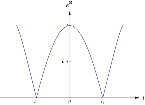
Examples of this case have been studied in the literature before, see e.g. Klaput:2011mz . This flow has also been studied more recently including corrections and the vector bundle over which comes with every heterotic string compactification Klaput:2013nla ; Haupt:2014ufa . Interestingly, it was shown in Klaput:2013nla that can have a finite volume as by choosing appropriately the bundle . It should be noted however that for the -corrected flow in Klaput:2013nla , the dilaton becomes -dependent. Moreover, for solutions where the internal radius tends to a constant, i.e. , the dilaton blows up as . The decompactification limit we found at zeroth order in is therefore traded for a finite volume compactification and a dilaton which blows up.
5.2 Flow with varying
The second solution to equation (116) is
Consider now the equation for (108). Changing variables using (114) we find
where we have used the relation
| (120) |
The sign in this relation is chosen by requiring consistency with equation (115). Integrating we now obtain
| (121) |
In the expression for , we note that must be positive in order for the right hand side to be positive. As a function of , is a monotonically decreasing function and as . The requirement that is a positive function means that for positive, we need to choose the positive sign in equation (114) and the negative sign in (120). Of course, for negative, we chose the opposite signs in these equations.
Finally we need to integrate equation (114) to find as a function of . Integrating the equation
we find
| (122) |
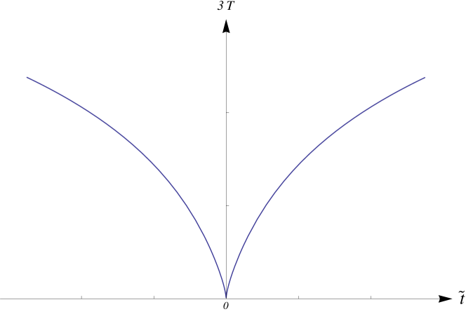
where , is a constant of integration, and is the incomplete Beta function. We choose the constant of integration so that when , that is , we set . Hence
We can always do this as this choice represents a constant shift in the values of . In Figure 3 we present a plot of as a function of .
The solution for the torsion class is
| (123) | ||||
| (124) |
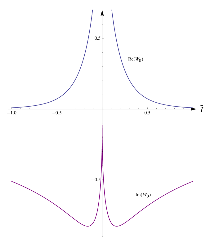
In Figure 4 we show the behaviour of with respect to . The torsion class as , however falls much faster than . In fact, as (or ) we find that
and hence
| (125) |
Finally, note that the point corresponds to a manifold with a curvature singularity as as .
It is interesting also to compute the variation of the dilaton. Recall that
Using equations (110) and (120), we find
and by equation (121)
Thus, the dilaton flows to a constant as .
Just as the case in the previous section, this solution flows to a non-compact Calabi–Yau manifold at . In this limit we have , , and the scalar curvature also vanishes . Moreover, both and increase monotonically to infinity, and hence the volume of at infinity is infinite.
This flow does not intersect the flow discussed in the previous section. The two cases only coincide at where they both flow into a non-compact Calabi–Yau manifold. However, the flow with varying approaches asymptotically the flow with constant when , as it is easily checked by comparing equation (125) with (117).
5.3 Appendix:
In this appendix we prove the claim at the beginning of this section that , or otherwise we fall back on a Calabi–Yau flow. Assume that
and consider the first Bianchi identity
where
Taking the wedge product with , and noting that is primitive, we find
For we must have
Note that this means that
| (126) |
as is a constant.
6 Half-flat structures
In this section we consider the flow of structures which are half-flat, that is when the torsion classes , vanish, but and are non-zero. As we will see below, Hitchin flow Hitchin:2000jd , for which the torsion classes of the manifold are all zero, is recovered as a subcase of this flow, with vanishing flux, constant dilaton and constant embedding functions . We will argue that simplified versions of half-flat flows can allow Calabi–Yau loci, even at finite values of . To conform with the previous sections, we choose .
A flow that preserves a half-flat structure should for all obey
| (127) | ||||
| (128) |
where
is a closed form. Taking the exterior derivative of equation (127) and (128) one finds differential equations for the torsion classes
| (129) |
The flow equations for in this case are
Since is -constant and for all , we find a constraint
| (130) |
This is similar to the nearly Kähler case, with the difference that need not be constant.
The flow equations for are
| (131) | ||||
| (132) |
To study the flow of structures, it is useful to record the -variations of the torsion classes. Compatibility between the flow equation for and the variation of equation (127), or equivalently, using equation (49) with and vanishing Lie forms, gives
| (133) |
Note that this equation satisfies
as required by the primitivity of . It should also satisfy
as required by the fact that is a three form of type . This constraint gives a flow equation for
| (134) |
Compatibility between the flow equation for and the variation of equation (128) gives a flow equation for
| (135) |
By assumption, the variation of the Lie forms is zero along a half-flat flow.
The first Bianchi identity is a constraint on the exterior derivative of . With
we have
| (136) |
Taking the wedge product of this equation with , and recalling that is primitive, we find
| (137) |
which will be of use below.
The second Bianchi identity, , where
determines, among other things, the flow of . For our discussion below, we will be particularly interested in the necessary constraints obtained by wedging the second Bianchi identity with and . From the former, we obtain
| (138) |
where we have used equation (137). From the latter we get
| (139) |
Note that (138) can be viewed as a differential equation for the dilaton , whereas (139) determines the one-form . Moreover, the right hand side of equation (138) is negative definite, hence it gives an inequality
| (140) |
which is saturated only when is a Calabi–Yau manifold.
Given the complexity of the flow equations (133)-(135) and the constraints from the Bianchi identities (136)-(139), we will not attempt to solve this system of equations in full generality. Instead, we proceed to study simplified cases, where we make assumptions on the flux and the embedding of the structure.
We begin by an inspection of the first Bianchi identity (136). This is a strong constraint on that completely determines its non-coclosed components. If we moreover assume that is coclosed, (136) immediately tells us that
| (141) |
and furthermore gives relations that determine the flow of the complex phase of and . Using this in equation (140) and (139), we derive the necessary constraints
where the first inequality can only be saturated when is a Calabi–Yau manifold as mentioned above.
It is interesting that the requirement that is coclosed has so far-reaching consequences for the structure and its embedding. Recall that in our first order analysis of flows away from a Calabi–Yau manifold , we showed that a half-flat structure was obtained when , but (cf. equation (86)). Although the flow of a half-flat structure with vanishing would be a natural guess for the completion of this first order flow, the constraint we just derived shows that this is not the case. A non-zero seems necessary in order for a half-flat flow to contain Calabi–Yau loci at finite values of .
Half-flat flows with coclosed have been studied before Hitchin:2000jd ; chiossi ; Gray:2012md ; Lukas:2010mf ; Klaput:2011mz ; Klaput:2012vv ; Klaput:2013nla . A particular case is Hitchin flow, where not only , but also and vanish, and the dilaton and embedding parameter are both constant. In this case, we can embed the half-flat structure in a holonomy manifold, and the flow equations can be summarised as
| (142) |
in the gauge where is taken to be constant.555Recall that when the two Lie forms vanish, we are free to choose the phase of without changing the properties of the structure. Thus, we can always choose a gauge where the real (imaginary) part of is closed, and hence are imaginary (real). Once we have fixed , these gauge choices correspond to different ways of embedding the structure in a structure. From our discussion above, it is clear that this flow cannot contain Calabi–Yau loci. This can also be seen as follows: and are closed at a Calabi–Yau locus, which means that the right-hand sides of the equations (142) vanish at that point of the flow. It is easy to see that the first order derivatives of the torsion classes (133)-(135) then also vanish. Moreover, a straightforward inductive analysis shows that all higher order -derivatives of the torsion classes vanish, and hence and have to remain closed along the flow. Consequently, Calabi–Yau manifolds are fix points of the Hitchin flow.
In order to connect first order analysis of the flow from a Calabi–Yau threefold in section 4.3, we therefore need flows where either the embedding parameter is non-constant and the flux is non-vanishing. In the next subsection, we analyse a simple type of such a flow.
6.1 Symplectic half-flat
There is a way to simplify the analysis of half-flat flows, that still allows to connect with the perturbative analysis of the Calabi–Yau flow. In section 4.3 we found that, at linear order, a Calabi–Yau manifold with constant and non-harmonic resulted in a symplectic half-flat structure with real , see equation (87). Therefore, let us now consider the flow of such structures, that is where
| (143) | ||||
| (144) |
Since is closed, it provides the six-manifold with a symplectic structure. As above, we will look for points along the flow where vanishes.
We begin by proving that
| (145) |
along this flow. To see this consider the flow of the torsion class , (134), for symplectic half-flat structures. The real and imaginary parts of this equation must vanish separately, so with for all we have
| (146) |
Taking the Hodge dual of the first equation we find
As the left hand side is -exact, and the right hand side is either strictly positive or strictly negative, this identity can only be true if both sides vanish. Hence, equation (145) follows. Recall that any -dependence of a -constant can be absorbed by a coordinate change. We will therefore take constant below.
The flow equations for become (note that )
with solution
| (147) |
The closure of is automatic, since we assume that is zero along the flow. Thus, requiring that is closed for all leads to no further constraints. This is consistent with the fact that the flow equation for , (133), is trivially satisfied along the flow.
The flow equations for are (note that )
| (148) |
For future reference, we record the compatibility conditions coming from :
| (149) |
Finally, the supersymmetry equations fix the flux to
| (150) |
As above, the first Bianchi identity is a constraint on the exterior derivative of , which can be read off from (136) after setting to zero. The second Bianchi identity determines the flow of with . The compatibility of these equations with (149) must be checked. First, we have
| (151) |
which is compatible with (149) if and only if
| (152) |
The second Bianchi identity gives, upon using (152),
| (153) |
Thus, given , the second Bianchi identity further constrains the flow of . This equation is difficult to solve in general, but we note that all terms in the last equation are -closed. Thus, the equation is compatible with the constraints on the flow.
Let us summarise the conditions for a symplectic half-flat flow. We have
| (154) |
and can rewrite (149) and (153) as constraints on :
| (155) |
Consider the wedge product with of the last equation (see equation (138))
As the left hand side is negative definite on a symplectic half-flat manifold, it must be the case that
| (156) |
Consequently, flows with constant dilaton are thus excluded for symplectic half-flat SU(3) structures: the inequality in (156) can only be saturated if and both vanish. This takes us back to a Calabi–Yau flow as discussed earlier.
The flow specified by the equations (155) depends on whether vanishes or not. We therefore have two different classes of solutions.
6.1.1
In the case that for all , which is in particular true if is zero, we can solve (155) explicitly. First, note that implies that and . The flow equations for and then integrate to
| (157) |
where a zero denotes the value of the form at some point along the flow, and . Clearly, there is no non-singular Calabi–Yau locus in this flow: if goes to zero, so do and , leading to a manifold of vanishing volume. As we discuss further below, this is consistent with the first order analysis of flows from Calabi–Yau manifolds.
The third equation of (155) can be decomposed into
| (158) |
where must be positive by (156). The first equation is a constraint on the structure of . The second equation is an non-linear differential equation for the flow of :
where is a positive constant. To solve this, we proceed as in the analysis of nearly Kähler flows (cf. section 5): let
| (159) |
In terms of the differential equation becomes
Substituting and we find a first order differential equation for . Substituting back, we can solve for . We have
Note that the right hand side of always negative irrespective of the sign one chooses for . Inverting this relation we obtain
| (160) |
where must be positive. Moreover, when taking the square root of this relation, one must take the absolute value of the cosine so that is always positive.
At infinitely many points , where and is an integer, we see that
| (161) |
Recalling the relations (157), we thus see that the volume of the structure manifold vanishes at regular intervals. However, this is no curvature singularity, since the scalar curvature is proportional to and hence goes to zero at these points. To follow the flow through these possibly singular points666It is possible that the manifold compactifies and stays regular when the structure fibre shrinks to zero size, in analogy with how a one-circle fibered over an interval forms a two-sphere by shrinking to zero size at the boundaries of the interval. requires an analysis that goes beyond the supergravity approximation used in this paper. Although corrections should still be small at , corrections might still be important. We hope to come back to this discussion in the future. For the present analysis, we will circumvent this discussion by focusing on the flow of in the domain .
Finally, to find as a function of , we solve equation (159). Substituting (160) into (159), we have
For values of in the domain , the integral gives
where is the elliptic function of the second kind. The range of is finite, and bounded by . By inverting this relation to get , we can plot the evolution of in the interval . The result is given in figure 5, where we have chosen and normalised so that .
6.1.2
A non-zero makes the equations (155) more intricate. Indeed, without recourse to the analysis of explicit examples, which goes beyond the scope of this paper, only a few qualitative observations can be made. First, the second equation in (155) clarifies that it is only when is non-closed, that can vanish at some point along the flow, without also going to zero. This is in agreement with the first order analysis of the flow away from Calabi–Yau, where we found that a non-closed was required to generate . In contrast to the nearly Kähler case discussed in section 5, there are no direct obstructions to being finite.777 However, to answer this question in ernest requires the analysis of example manifolds with . On such spaces, can be explicitely computed, and various ansätze for can be tested. We hope to come back to such an analysis in the future.
Second, we recall (156) which shows that symplectic half-flat flows require a non-constant at least for some range of , in order not to fall back into a Calabi–Yau flow for all . This constraint requires that is a concave function of . As such, it will cross the -axis at at least one point, and at these point the structure of is singular, since its volume goes to zero.
Finally, it should be mentioned that it is still allowed that asymptotes to a linear, or even a constant function for some . Concretely, suppose that the strict inequality (156) holds for , but is saturated after : the symplectic half-flat manifold would then flow to a Calabi–Yau manifold without flux, with volume proportional to . However, to keep the dilaton evolution smooth, it is likely that the transition will be asymptotic, and the point will be at infinity. We thus conclude that non-singular Calabi–Yau loci at finite require the presence of flux, and in particular a non-vanishing .
7 Conclusions
In this paper, we have been concerned with heterotic string compactifications to a four-dimensional non-compact space that is is not maximally symmetric. To be more precise, we have focused on four-dimensional half-BPS domain wall compactifications. We saw that by allowing for a non-maximally symmetric spacetime, the internal six-dimensional space is in general torsional, even at zeroth order in . The compact geometry is, however, always a manifold with structure.
This paper is a continuation of an ongoing program that strives to get a better understanding of heterotic string compactifications to non-maximally symmetric spacetimes Lukas:2010mf ; Klaput:2011mz ; Gray:2012md ; Klaput:2012vv ; Klaput:2013nla ; Larfors:2013zva ; Maxfield:2014wea ; Gurrieri:2004dt ; Micu:2004tz ; deCarlos:2005kh ; Gurrieri:2007jg ; Micu:2009ci ; Haupt:2014ufa ; Held:2010az ; Held:2011uz ; Chatzistavrakidis:2012qb . The physical motivation for these studies is that such compactifications might, after inclusion of non-perturbative effects, complete to phenomenologically relevant four-dimensional models. Mathematically, one goal of this program is to get a better understanding of the moduli space of the structures that arise in flux compactifications. This is a very hard question in general. For instance, the usual cohomological tools available for the analysis of the moduli space of Calabi–Yau compactifications no longer apply, or at least require modifications, due to the torsional nature of the compact space.
By focusing on domain wall compactifications, the structure can be embedded into a non-compact seven-dimensional structure. Such an embedding corresponds to a flow along a path in the structure moduli space, thus facilitating the analysis of some of the features of this space. In this paper, we investigated how restrictive the embedding is when selecting these paths. For example, is it possible to flow from one structure with a certain type of torsion classes, to another with different torsion classes turned on? By considering both structure preserving and changing flows, we showed by examples that the answer to this question is yes. In particular, we derived the constraints for a embedding to preserve structures of Calabi–Yau and nearly Kähler type. In both cases, we found that restrictions only apply to a function , which encodes warping in the metric, and a primitive (2,1)-form , that is part of the -flux in the configuration. Through a perturbative analysis of the Calabi–Yau flow to linear order, we showed that if the constraints on and are violated, torsion classes are switched on by the flow.
Additionally, we have analysed the flows of nearly Kähler and half-flat structures, and provided evidence that both contain Calabi–Yau loci. For nearly Kähler manifolds, where we solved the flow equations explicitly, these loci are necessarily in the limit where goes to infinity. For half-flat manifolds, we found support for the existence of Calabi–Yau loci also at finite distance, but due to the complexity of the equations in this case, we cannot present a definite answer to this question. Nevertheless, this does not render the analysis void, as we have discovered attributes to the flow, necessary for consistent non-Calabi–Yau solutions. For example, it seems that at least one singularity or “domain wall” is required along the flow. It would be interesting to find a physical interpretation of these walls, possibly in terms of NS5-branes and Kaluza–Klein monopoles.
From a physics perspective, the relaxation of constraints on the compact geometry can be understood since there is less supersymmetry, and hence more freedom, in the compactification compared with the maximally symmetric case. Still, the structure embedding is under enough control to provide a fertile ground for the study of string compactifications and the moduli space of structures in general. Our study has uncovered some features of these spaces, but many intriguing questions remain for future studies.
These include further investigations of the integrability of flows that connect Calabi–Yau and non-Calabi–Yau manifolds, for example by extending our perturbative analysis to higher orders. It would also be interesting to study the flow of specific examples of structure manifolds with known torsion classes. Our results indicate that symplectic half-flat manifolds are particularly relevant, as they are simple but might still flow to Calabi–Yau manifolds at finite distance. A study of the flow of smooth compact toric varieties with structure, that have been constructed in Larfors:2010wb ; Larfors:2011zz ; Larfors:2013zva , might also be rewarding.
Another area to explore is whether the torsion-changing flows we find also change the topology of the six-dimensional manifold. From our analysis, there are no indications of this: what seems to happen is that different structures on the same topological space flow into each other. However, many flows contain singularities where the volume of the compact space goes to zero, and where the scalar curvature either goes to zero or infinity. In this paper, we have refrained from studying the flow through such points, but we cannot avoid noting the similarities with conifold points in Calabi–Yau moduli spaces, and how they smoothly connect different moduli spaces Candelas:1989js ; Strominger:1995cz ; Chen:2010ssa . Topology-changing Calabi–Yau flows have recently been shown to be relevant in the study of two-dimensional supersymmetric theories Gadde:2013sca . The flows studied here might find similar applications.
In the present paper, we have analysed heterotic compactifications at zeroth order in . It is known that effects at linear order in can change the flow quite drastically for certain structure manifolds, see e.g. Klaput:2012vv ; Haupt:2014ufa . Indeed, such effects couple the gauge and gravity sectors of heterotic supergravity, leading to a more intricate mathematical problem. It would be interesting to see how these effects impact on the findings of the present paper. A relatively straightforward study would be to extend the analysis of Klaput:2012vv ; Haupt:2014ufa to the phase-changing flow of nearly Kähler manifolds that we discussed in section 5.
Furthermore, in order to properly include the gauge sector, a modified description of the heterotic configuration might be required. In delaOssa:2014cia ; Anderson:2014xha ; delaOssa:2014msa it was shown that maximally symmetric heterotic compactifications to six dimensions can be encoded in a holomorphic structure on a certain extension bundle. This structure also relates to the generalised geometric description of the heterotic string Garcia-Fernandez:2013gja ; Baraglia:2013wua ; Bedoya:2014pma ; Coimbra:2014qaa . Moreover, by rephrasing the whole system in terms of a holomorphic structure, it was possible to compute the first order moduli space in the maximally symmetric case. This is done by means of cohomologies of the holomorphic structures involved. It may be that similar structures are required when considering the corrected domain wall compactifications. However, since in this case the base space of the bundle is non-complex in general, these structures will no longer be holomorphic. The framework would therefore have to be generalised to apply to the domain wall case. Hints for such a generalisation might be found in recent studies of cohomologies for flux compactifications of type II supergravities Tseng:2011gv , and it would be interesting to study this in more detail in the future.
Acknowledgements
The authors thank Thomas Bruun Madsen, Philip Candelas, Diego Conti, Tudor Dimofte, Iñaki Garcia-Extebarria, James Gray, Spiro Karigiannis and Simon Salamon for interesting discussions over the course of this project. XD would like to acknowledge the hospitality of Perimeter Institute where part of this project was undertaken. ML would like to thank the University of Oxford for hospitality during the completion of this work. XD’s research was supported in part by the EPSRC grant BKRWDM00. The research of ML was supported by the Swedish Research Council (VR) under the contract 623-2011-7205. ES was supported by the Clarendon Scholarship of OUP, and a Balliol College Dervorguilla Scholarship. Part of ES’s work was also made in the ILP LABEX (under reference ANR-10-LABX-63), and was supported by French state funds managed by the ANR within the Investissements d’Avenir programme under reference ANR-11-IDEX-0004-02.
Appendix A Conventions and identities
In this appendix we collect our conventions and some useful identities. Our conventions conform with those of huybrechts .
Index conventions: we use latin indices for real indices, and greek indices for holomorphic indices.
Torsion:
A.1 Differential forms and wedge products
A -form is defined by
| (162) |
The wedge product between a -form and a -form is
| (163) |
A.2 Hodge operator and the adjoint operator
Let be a -form. The Hodge operator on for a -dimensional manifold is defined by
| (164) |
Then if is even,
and if is odd
In general,
| (165) |
The adjoint operator on is defined by
| (166) |
If is even, then
and if is odd
A.3 Contraction operator
The operator denotes the contraction of forms, and is defined by
| (167) |
where is any -form and is any -form. It is easy to deduce the identity
| (168) |
A.4 Conventions on almost complex manifolds
Real and complex coordinates: We define complex coordinates
and is the real dimension of the manifold.
Hermitian form:
In complex coordinates . We have the identity
| (169) |
Almost complex structure and projection operators
Let be a -form. The almost complex structure acts on a form as follows
| (170) |
The projection operators
| (171) |
project a 1-form onto its holomorphic and antiholomorphic components, respectively.
Volume form
Hodge operator
Let be a primitive -form. Then, with ,
| (172) |
Let be a one form. Then
| (173) |
This identity is a “non-Kähler identity” and reduces to one of the Kähler identities when is -closed.
Identitites in 6 dimensions
Holomorphic volume form
Any almost complex 6-manifold has a nowhere-vanishing holomorphic top form, defined by
The following identities hold
| (174) | ||||
Note that ; together and determine an structure. We also have
Useful identies
Let be a -form
| (175) |
Let be a 1-form
| (176) |
Let be a 2-form
| (177) |
Let be a 3-form
| (178) |
Identities involving a closed holomorphic -form
Let be a function
| (179) |
Let be a two-form
| (180) |
Calabi–Yau identities: On a Calabi–Yau manifold, we have
| (181) |
Let be a function. Then
| (182) |
The almost complex structure in terms of : The (real part of the) complex 3-form determines a unique almost complex structure such that is a -form with respect to ,
| (183) |
The variations of in terms of the variations of are given by
| (184) |
A.5 Conventions on 7-dimensional manifolds
Let be the 3-form that determines the structure. Then
| (185) |
Let be a -form with
then
| (186) |
References
- (1) P. Candelas, G. T. Horowitz, A. Strominger, and E. Witten, Vacuum Configurations for Superstrings, Nucl.Phys. B258 (1985) 46–74.
- (2) A. Strominger, Superstrings with Torsion, Nucl.Phys. B274 (1986) 253.
- (3) C. Hull, Compactifications of the Heterotic Superstring, Phys.Lett. B178 (1986) 357.
- (4) D. Lüst, Compactification of Ten-dimensional Superstring Theories Over Ricci Flat Coset Spaces, Nucl.Phys. B276 (1986) 220.
- (5) K. Dasgupta, G. Rajesh, and S. Sethi, M theory, orientifolds and G - flux, JHEP 9908 (1999) 023, [hep-th/9908088].
- (6) S. Ivanov and G. Papadopoulos, A No go theorem for string warped compactifications, Phys.Lett. B497 (2001) 309–316, [hep-th/0008232].
- (7) K. Becker and K. Dasgupta, Heterotic strings with torsion, JHEP 0211 (2002) 006, [hep-th/0209077].
- (8) K. Becker, M. Becker, P. S. Green, K. Dasgupta, and E. Sharpe, Compactifications of heterotic strings on nonKahler complex manifolds. 2., Nucl.Phys. B678 (2004) 19–100, [hep-th/0310058].
- (9) K. Becker, M. Becker, K. Dasgupta, and P. S. Green, Compactifications of heterotic theory on nonKahler complex manifolds. 1., JHEP 0304 (2003) 007, [hep-th/0301161].
- (10) J. P. Gauntlett, D. Martelli, S. Pakis, and D. Waldram, G structures and wrapped NS5-branes, Commun.Math.Phys. 247 (2004) 421–445, [hep-th/0205050].
- (11) G. Lopes Cardoso, G. Curio, G. Dall’Agata, D. Lüst, P. Manousselis, et. al., NonKahler string backgrounds and their five torsion classes, Nucl.Phys. B652 (2003) 5–34, [hep-th/0211118].
- (12) J. P. Gauntlett, D. Martelli, and D. Waldram, Superstrings with intrinsic torsion, Phys.Rev. D69 (2004) 086002, [hep-th/0302158].
- (13) U. Gran, P. Lohrmann, and G. Papadopoulos, The Spinorial geometry of supersymmetric heterotic string backgrounds, JHEP 0602 (2006) 063, [hep-th/0510176].
- (14) M. Becker, L.-S. Tseng, and S.-T. Yau, Moduli Space of Torsional Manifolds, Nucl.Phys. B786 (2007) 119–134, [hep-th/0612290].
- (15) U. Gran, G. Papadopoulos, and D. Roest, Supersymmetric heterotic string backgrounds, Phys.Lett. B656 (2007) 119–126, [arXiv:0706.4407].
- (16) S. Ivanov, Heterotic supersymmetry, anomaly cancellation and equations of motion, Phys.Lett. B685 (2010) 190–196, [arXiv:0908.2927].
- (17) N. J. Hitchin, The geometry of three-forms in six and seven dimensions, math/0010054.
- (18) S. Chiossi and S. Salamon, The intrinsic torsion of SU(3) and G_2 structures, ArXiv Mathematics e-prints (Feb., 2002) [math/0202].
- (19) M. Graña, Flux compactifications in string theory: A Comprehensive review, Phys.Rept. 423 (2006) 91–158, [hep-th/0509003].
- (20) R. Blumenhagen, B. Kors, D. Lüst, and S. Stieberger, Four-dimensional String Compactifications with D-Branes, Orientifolds and Fluxes, Phys.Rept. 445 (2007) 1–193, [hep-th/0610327].
- (21) P. Koerber, Lectures on Generalized Complex Geometry for Physicists, Fortsch.Phys. 59 (2011) 169–242, [arXiv:1006.1536].
- (22) M. Larfors, Revisiting toric SU(3) structures, Fortsch.Phys. 61 (2013) 1031–1055, [arXiv:1309.2953].
- (23) J. Gray, M. Larfors, and D. Lüst, Heterotic domain wall solutions and SU(3) structure manifolds, JHEP 1208 (2012) 099, [arXiv:1205.6208].
- (24) A. Lukas and C. Matti, G-structures and Domain Walls in Heterotic Theories, JHEP 1101 (2011) 151, [arXiv:1005.5302].
- (25) M. Klaput, A. Lukas, and C. Matti, Bundles over Nearly-Kahler Homogeneous Spaces in Heterotic String Theory, JHEP 1109 (2011) 100, [arXiv:1107.3573].
- (26) M. Klaput, A. Lukas, C. Matti, and E. E. Svanes, Moduli Stabilising in Heterotic Nearly Kähler Compactifications, JHEP 1301 (2013) 015, [arXiv:1210.5933].
- (27) M. Klaput, A. Lukas, and E. E. Svanes, Heterotic Calabi-Yau Compactifications with Flux, JHEP 1309 (2013) 034, [arXiv:1305.0594].
- (28) S. Gurrieri, A. Lukas, and A. Micu, Heterotic on half-flat, Phys.Rev. D70 (2004) 126009, [hep-th/0408121].
- (29) A. Micu, Heterotic compactifications and nearly-Kahler manifolds, Phys.Rev. D70 (2004) 126002, [hep-th/0409008].
- (30) B. de Carlos, S. Gurrieri, A. Lukas, and A. Micu, Moduli stabilisation in heterotic string compactifications, JHEP 0603 (2006) 005, [hep-th/0507173].
- (31) S. Gurrieri, A. Lukas, and A. Micu, Heterotic String Compactifications on Half-flat Manifolds. II., JHEP 0712 (2007) 081, [arXiv:0709.1932].
- (32) A. Micu, Moduli Stabilisation in Heterotic Models with Standard Embedding, JHEP 1001 (2010) 011, [arXiv:0911.2311].
- (33) P. Candelas and X. de la Ossa, Moduli Space of Calabi-Yau Manifolds, Nucl.Phys. B355 (1991) 455–481.
- (34) L.-S. Tseng and S.-T. Yau, Cohomology and Hodge Theory on Symplectic Manifolds. I., J.Diff.Geom. 91 (2012) 383–416, [arXiv:0909.5418].
- (35) L.-S. Tseng and S.-T. Yau, Cohomology and Hodge Theory on Symplectic Manifolds. II, J.Diff.Geom. 91 (2012) 417–444, [arXiv:1011.1250].
- (36) L.-S. Tseng and S.-T. Yau, Generalized Cohomologies and Supersymmetry, arXiv:1111.6968.
- (37) L. B. Anderson, J. Gray, and E. Sharpe, Algebroids, Heterotic Moduli Spaces and the Strominger System, arXiv:1402.1532.
- (38) X. de la Ossa and E. E. Svanes, Holomorphic Bundles and the Moduli Space of N=1 Supersymmetric Heterotic Compactifications, arXiv:1402.1725.
- (39) X. de la Ossa, S. Karigiannis, and E. E. Svanes To appear.
- (40) M. Fernandez and A. Gray, Riemannian manifolds with structure group g2, Ann. Mat. Pura Appl. 32 (1982) 19–45.
- (41) T. Friedrich and S. Ivanov, Killing spinor equations in dimension 7 and geometry of integrable G2-manifolds, Journal of Geometry and Physics 48 (Oct., 2003) 1–11, [math/0112201].
- (42) D. Martelli and J. Sparks, Non-Kahler heterotic rotations, Adv.Theor.Math.Phys. 15 (2011) 131–174, [arXiv:1010.4031].
- (43) A. Gray and L. Hervella, The sixteen classes of almost hermitian manifolds and their linear invariants, Annali di Matematica Pura ed Applicata 123 (1980), no. 1 35–58.
- (44) N. Hitchin, Stable forms and special metrics, in Global differential geometry: the mathematical legacy of Alfred Gray (Bilbao, 2000), number 288 in Contemp. Math, pp. 70–89, 2001.
- (45) K. Kodaira and D. C. Spencer, On deformations of complex analytic structures. I, II, Ann. of Math. (2) 67 (1958) 328–466.
- (46) K. Kodaira and D. Spencer, On deformations of complex analytic structures. III: Stability theorems for complex structures., Ann. Math. (2) 71 (1960) 43–76.
- (47) G. Tian, Smoothness of the universal deformation space of compact calabi-yau manifolds and its petersson-weil metric, in Mathematical aspects of string theory (San Diego, Calif., 1986), Adv. Ser. Math. Phys., pp. 629–646, World Sci. Publishing, Singapore, 1986.
- (48) A. S. Haupt, O. Lechtenfeld, and E. T. Musaev, Order heterotic domain walls with warped nearly Kähler geometry, arXiv:1409.0548.
- (49) L. Bedulli and L. Vezzoni, The Ricci tensor of SU(3)-manifolds, Journal of Geometry and Physics 57 (Mar., 2007) 1125–1146, [math/0606].
- (50) T. Maxfield and S. Sethi, Domain Walls, Triples and Acceleration, JHEP 1408 (2014) 066, [arXiv:1404.2564].
- (51) J. Held, D. Lüst, F. Marchesano, and L. Martucci, DWSB in heterotic flux compactifications, JHEP 1006 (2010) 090, [arXiv:1004.0867].
- (52) J. Held, BPS-like potential for compactifications of heterotic M-theory?, JHEP 1110 (2011) 136, [arXiv:1109.1974].
- (53) A. Chatzistavrakidis, O. Lechtenfeld and A. D. Popov, Nearly Kähler heterotic compactifications with fermion condensates, JHEP 1204 (2012) 114 [arXiv:1202.1278].
- (54) M. Larfors, D. Lüst, and D. Tsimpis, Flux compactification on smooth, compact three-dimensional toric varieties, JHEP 1007 (2010) 073, [arXiv:1005.2194].
- (55) M. Larfors, Flux compactifications on toric varieties, Fortsch.Phys. 59 (2011) 730–733.
- (56) P. Candelas and X. C. de la Ossa, Comments on Conifolds, Nucl.Phys. B342 (1990) 246–268.
- (57) A. Strominger, Massless black holes and conifolds in string theory, Nucl.Phys. B451 (1995) 96–108, [hep-th/9504090].
- (58) F. Chen, K. Dasgupta, P. Franche, and R. Tatar, Toward the Gravity Dual of Heterotic Small Instantons, Phys.Rev. D83 (2011) 046006, [arXiv:1010.5509].
- (59) A. Gadde, S. Gukov, and P. Putrov, Fivebranes and 4-manifolds, arXiv:1306.4320.
- (60) X. de la Ossa and E. E. Svanes, Connections, Field Redefinitions and Heterotic Supergravity, arXiv:1409.3347.
- (61) M. Garcia-Fernandez, Torsion-free generalized connections and Heterotic Supergravity, arXiv:1304.4294.
- (62) D. Baraglia and P. Hekmati, Transitive Courant Algebroids, String Structures and T-duality, arXiv:1308.5159.
- (63) O. A. Bedoya, D. Marques, and C. Nunez, Heterotic ’-corrections in Double Field Theory, arXiv:1407.0365.
- (64) A. Coimbra, R. Minasian, H. Triendl, and D. Waldram, Generalised geometry for string corrections, arXiv:1407.7542.
- (65) D. Huybrechts, Complex Geometry An Introduction. Springer, 2005.