Mass spectral analysis and quantification of Secondary Ion Mass Spectrometry data

Abstract

This work highlights the possibility of improving the quantification aspect of Cs-complex ions in SIMS (Secondary Ion Mass Spectrometry), by combining the intensities of all possible Cs-complexes. Identification of all possible Cs-complexes requires quantitative analysis of mass spectrum from the material of interest. The important steps of this mass spectral analysis include constructing fingerprint mass spectra of the constituent species from the table of isotopic abundances of elements, constructing the system(s) of linear equations to get the intensities of those species, solving them, evaluating the solutions and employing a regularization process when required. These steps are comprehensively described and the results of their application on a SIMS mass spectrum obtained from D9 steel are presented. It is demonstrated that results from the summation procedure, which covers entire range of sputtered clusters, is superior to results from single Cs-complex per element. The result of employing a regularization process in solving a mass spectrum from an SS316LN steel specimen is provided to demonstrate the necessity of regularization.

1 Introduction

Knowledge of chemical composition is an important aspect in the study of materials. As a surface analytical technique, Secondary Ion Mass Spectrometry (SIMS), is employed for composition profiling of materials in widely varying fields like semiconductor industry[1] and nuclear technology[2, 3]. This technique has high sensitivity, surface specificity, and high dynamic range. However, it lacks quantification because of the dependence of yield of secondary ions on the composition (matrix) of the surface from which it is ejected.[4, 5] This artefact of the technique is called as matrix effect. In semiconductor industry, the number of commonly analyzed semiconductor materials is limited. Hence, semiconductor research uses matrix-matched standards to quantify SIMS measurements.[6] However, in a general case, like a compound multilayer or an alloy with oxidized surface, the composition is likely to vary over a vast range in the volume analyzed. Such specimens would require a very large number of standards matching each of those compositions to quantify the data. Hence, employing matrix-matched standards in such cases is near to impossible. The matrix effect in the intensities of XCs${}_{n}^{+}$ secondary ions measured with Cs⁺ primary ions (where X stands for an atom from the specimen and n is equal to 1 or 2) was shown by Gao [7, 8] to be much lower (in some cases, even by orders of magnitude) than that in secondary elemental ions. However, there is considerable deviation of the composition computed from these XCs_n signals from the actual composition. In spite of developments in understanding the formation process of these species (for example, ref [9, 10, 11, 12, 13, 14, 15, 16, 17]), a gap remains in this approach in reaching complete quantification. The current work provides an incremental step in filling this gap.

2 Theory

The XCs⁺ secondary ions are understood to be formed by the combination of a resputtered Cs⁺ ion with a sputtered neutral atom from the specimen [9, 10, 11, 12, 13, 14, 15, 16, 17]. Since secondary neutrals are formed as different atomic clusters[17, 18, 19, 20], the intensities of the Cs complexes of all these clusters should be combined to enhance the quantitativeness of XCs SIMS. This was earlier verified with a limited number of Cs complexes [21]. However, testing this with all the Cs complexes involves quantitative measurement of the intensities of the species constituting a mass spectrum and then computing the composition from those intensities.

3 Material and Methods

In this report, the details of this process are presented by analyzing a mass spectrum obtained from a sample of D9 steel, produced by M/s. Valinox, France. D9 is the steel used in fast reactors as a construction material of core components because of its resistance to void swelling.[3] It was selected as a material for test in this report, because it is a multi-component alloy with known composition. The implementation of the above theory involves setting up and solving systems of linear equations to know the composition of the mass spectrum. A mass spectrum is analyzed completely by considering its peaks one after another. With a peak chosen for analysis, a probable species with its mono-isotopic mass equal to the mass of that peak is first identified. This species could be mono atomic or a poly atomic cluster. Its fingerprint mass spectrum has to be constructed and matched with the experimental mass spectrum. If this species contains $n$ number of elements, the number $N$ of different isotopic combinations forming this species is given by

$$N=\prod_{i=1}^{n}\frac{(r_{i}+s_{i}-1)!}{r_{i}!(s_{i}-1)!}$$ (1)

where $r_{i}$, is the number of atoms of the $i^{th}$ element in the species and $s_{i}$ is the number of isotopes of the $i^{th}$ element. Those isotopic combinations with differences in mass, which are not discernible by the resolving power of the mass analyzer, appear as a single peak in the mass spectrum. (For example, in the cluster species CrFe, the combinations, ⁵⁴Cr⁵⁴Fe and ⁵²Cr⁵⁶Fe differ by a mass of 0.003u. A typical mass spectrometer with mass resolving power (MRP) of 500 cannot resolve these two combinations since the MRP required to resolve these species is 35428.) Hence, generally in a mass spectrum, the number of peaks corresponding to a cluster species is fewer than $N$. This group of peaks from the mass spectrometer forms the fingerprint spectrum of the species after normalizing the sum of their intensities to unity.

The fingerprint spectra of many species are likely to overlap with each other. The difficulty of identifying and measuring the intensities of such species in the measured spectrum depends on the number and complexity of their fingerprint spectra. The overlapping fingerprint spectra in the measured spectrum are mathematically represented by a system of linear equations. This system of equations contains one equation for every peak in the spectrum that is the resultant of overlap. For $q$ number of species, overlapping with each other, constituting $p$ number of peaks, the system of equations is

$$\sum_{j=1}^{q}a_{ij}s_{j}+\delta_{i}=m_{i}$$ (2)

where $i$ runs from $1$ to $p$ representing the $p$ number of equations and $m_{i}$ is the measured intensity of the $i^{th}$ peak. $s_{j}$ is the intensity of the $j^{th}$ species, to be solved for. If the fingerprint mass spectrum of the $j^{th}$ species has a peak at the mass of the $i^{th}$ peak, $a_{ij}$ is the intensity of that peak of the fingerprint mass spectrum. Otherwise, $a_{ij}$ is zero. $\delta_{i}$ is the noise that occurred while measuring $m_{i}$, which is not known. This term was added for completeness of mathematical description. However, the above set of equations has to be solved without the knowledge of this term. The above set of equations can be represented in matrix form, after neglecting the noise term as,

$$\mathbf{A\ s=m}$$ (3)

where $\mathbf{A}$ is the $p\times q$ matrix containing the elements $a_{ij}$ of eqn.2. $\mathbf{s}$ is the $q\times 1$ solution vector and $\mathbf{m}$ is the $p\times 1$ input vector containing $s_{j}$ and $m_{i}$ of eqn.2 as their elements respectively. The solution providing the least squared deviation between the L.H.S. and R.H.S. of the above equation is obtained by solving the normal form of the above equation,

$$\mathbf{A^{T}\ A\ s}=\mathbf{A^{T}\ m}$$ (4)

where $\mathbf{A^{T}A}$ is a $p\times p$ matrix and $\mathbf{A^{T}m}$ is a $p\times 1$ vector. $\mathbf{A^{T}}$ means transpose of $\mathbf{A}$.

In a few circumstances, the solution may turn out to be erroneous (including negative values for the intensities of a few species) due either to the intensity of noise or to wrong choice of species or both. If the error in the solution is due to the noise in the data, the solution can be optimized by following a regularization algorithm such as the iterative algorithm discussed by Gautier et al[22, 23] to deconvolve instrumental broadening from SIMS depth profiles. The convolution matrix, solution of deconvolution and measured depth profile found in Ref. [22, 23] are to be replaced by the isotope abundance matrix $\mathbf{A}$, solution for intensities $\mathbf{s}$ and the measured mass spectrum $\mathbf{m}$ respectively to regularize the solution of eqn 3. Out of the two regularization conditions imposed in Ref. [22, 23], the condition of positivity has to be retained while rejecting the condition of smoothness since the intensities need not vary smoothly from species to species. If the choice of species is wrong, the intensities of one or more species in the solution may remain to be negative even after the regularization process. In such cases, other probable species have to be tried out and the process has to be repeated until all the correct species are identified.

The concentration of an element is computed as the fraction of the number of atoms of that element in the Cs complexes to the total number of atoms in all of the Cs complexes excluding atoms of Cs and any other element like O that might originate from the instrument,

$$c_{i}=\frac{\sum_{j=1}^{m}n_{ji}s_{j}}{\sum_{k=1}^{n}\sum_{l=1}^{e_{k}}n_{lk}s_{k}}$$ (5)

where $c_{i}$ is the concentration of the $i^{th}$ element, $m$ is the number of species containing the $i^{th}$ element, $n_{ji}$ is the number of atoms of $i^{th}$ element in the $j^{th}$ such species, $s_{j}$ is the intensity of that ($j^{th}$) species, $n$ is the total number of species identified, $e_{k}$ is the number of elements (excluding Cs and any other element as mentioned above) in the $k_{th}$ species, $n_{lk}$ is the number of atoms of the $l_{th}$ element in the $k^{th}$ species and $s_{k}$ is the intensity of the $k_{th}$ species.

The process of identifying and measuring the intensities of the species constituting a mass spectrum will be discussed here with a SIMS mass spectrum obtained from a D9 specimen. This mass spectrum was obtained using a SIMS (Cameca ims-4f) system by employing a $20\ nA$, $5.5\ keV$ $Cs^{+}$ primary ion beam for sputtering the specimen. The primary ion beam was rastered over a square area of width $150\ \mu m$ and the secondary ions were collected from the central circular area of diameter $33\ \mu m$. The mass spectrometer was operated with a mass resolving power of $500$ and energy band-pass of $125\ eV$ for the secondary ions . Eleven data points were recorded around each integral mass number to construct the peaks. A portion of the raw mass spectrum in addition to the peak values as calculated below is shown in figure 1.

4 Calculation

The SIMS mass spectral peaks have the shape of the convolution of the ion-beam crossover with the exit slit of the mass analyzer. The data required for analysis are the heights of these peaks. Since the data is subject to noise and the peaks have a sparse density of data, the highest raw data point of many of the peaks do not represent the apex position. Hence, the spectrum was smoothened by 3-point weighted average with the central point receiving a weight of 50% and the neighboring points a weight of 25%. After smoothening, the heights of the peaks decreased proportionately and almost all of the peaks obtained a unique apex point as shown in the figure. The apex values of most of the smoothened peaks could be considered as the heights of the respective peaks. The heights of the remaining peaks were estimated manually. The peak values so estimated are shown as a bar graph in figure 2.

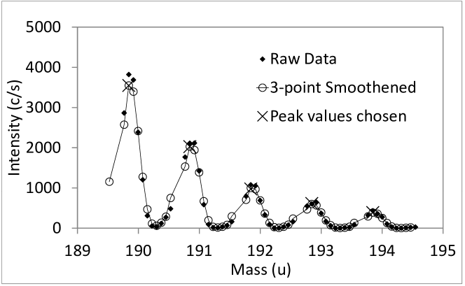
Figure 1: A portion of raw mass spectrum showing extraction of peak values

Figure 2: The mass spectrum over the complete mass range, constructed using the peak values picked up from the raw mass spectrum. The names of a few of the prominent species are labeled to the corresponding peaks.

The two strongest peaks in this mass spectrum, at mass numbers 133u and 266u, are those of Cs and Cs₂ respectively. The next highest peak is at mass number, 189u that is the mass of ⁵⁶Fe¹³³Cs. Setting up and solving eqn.3 for FeCs alone results in a slightly higher estimate for the intensity of FeCs, to minimize the squared deviation from the measured intensity at mass number 187u that is the mass of ⁵⁴Fe¹³³Cs as well as that of ⁵⁴Cr¹³³Cs. The higher estimate for FeCs compensates the absence of ⁵⁴Cr¹³³Cs in the equation for mass number 187u. After including CrCs in the equation, this error in the estimate for FeCs is corrected. In this manner, the probable species contributing to all the peaks can be tried out one after the other until all the peaks are successfully characterized. The final solution is not affected by the order in which the the peaks of the mass spectrum are chosen for analysis.

5 Results and Discussion

In the above mass spectrum, twenty four species were identified overlapping with each other spanning over the mass range from 177u to 208u, as shown in figure 3. In this figure, the measured spectrum is shown wider in the background and the constituent fingerprint spectra multiplied by their respective intensities are shown narrower in the foreground. With the perfect solution, the sum of the constituent spectra should be as equal to the measured spectrum as possible as shown in figure 3. The analysis of the complete mass spectrum resulted in identification of 165 species that are tabulated in Table 1. Most of them are Cs complexes that are required for the proposed quantification process.

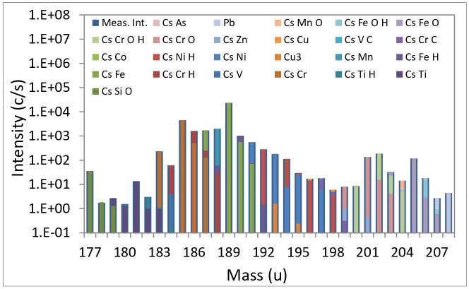
Figure 3: A portion of the complete mass spectrum shown in figure 2, labelled here as “Meas. MS”, and its composition computed using eqn 4

Species	Intensity (c/s)	Species	Int. (c/s)	Species	Int. (c/s)
Cs	23732613.0	Cr O H Cs2	13.70	Fe Ni O Cs2	3.17
Cs2	1745702.5	Fe Cr O Cs2	13.47	C	2.93
Fe Cs	25458.3	Mn	13.12	Cr Fe H Cs	2.86
Cr Cs	5328.6	Cr C Cs	12.86	Cr O2H Cs2	2.78
Ni Cs2	2749.8	Mo O H Cs	10.41	Ti H Cs	2.77
Fe Cs2	2094.4	Al Cs	10.15	Ni O Cs2	2.77
Mn Cs	1919.7	Fe Cr Cs2	9.62	Fe Cr N	2.72
Cr Cs2	1892.2	Si H Cs2	9.58	Cu	2.64
H Cs2	1790.9	Cr Ni Cs	9.42	Fe H	2.58
Cr H Cs	1311.1	O H Cs	9.08	Zn Cs	2.34
Ni Cs	685.7	O3	8.35	V O Cs2	2.32
Cs3	574.3	H Cs	8.16	Al2	2.19
Fe H Cs	511.6	Mn O Cs	8.15	Fe2O Cs	2.14
O H Cs2	507.7	O	8.14	Cr C N Cs2	2.01
Ni H Cs	402.5	Cu3	8.10	W Cs	2.00
Cr	352.8	O Cs	8.07	Fe O2Cs	1.94
O Cs2	315.6	Pb	8.05	Fe2O	1.82
Cr O H Cs	204.6	Ni C Cs2	8.01	Cr O2Cs	1.81
Cl Cs2	197.4	Mo H Cs2	7.97	Mn O Cs2	1.80
Fe	186.2	Ni Cr Cs2	7.35	V	1.72
Na	169.3	Si	6.60	Cu2	1.54
Fe H Cs2	167.4	Fe2O Cs2	6.54	Al Cs2	1.53
Cr O Cs	160.5	Co Cs	6.53	Cr O N Cs2	1.51
Mo Cs	155.1	Na2	6.46	O2	1.39
Cr O Cs2	144.1	Zn	6.44	Cr2	1.37
Si Cs2	139.6	Fe Ni Cs	5.72	Cr Mn O	1.29
Fe O Cs	128.1	Cs H2	5.41	Ni2O Cs2	1.25
Fe O Cs2	114.2	Cr Fe O Cs	5.37	Na Cs	1.24
Mo H Cs	107.1	Fe Cr O	5.27	Fe Cu	1.24
Ni H Cs2	74.7	Fe Ni H Cs2	5.25	S Cs2	1.10
Ti C Cs2	63.8	F Cs2	5.22	O H2Cs2	0.99
Mo Cs2	59.1	Co Cs2	5.07	P Cs2	0.94
K	54.8	Fe2H Cs2	5.02	O H	0.87
Si Cs	49.9	Cr2Cs	5.00	N	0.87
Fe2Cs2	43.2	Fe Cr	4.70	As Cs2	0.86
Si O Cs	38.8	Ti H	4.61	C H	0.85
Al	35.1	Ni2Cs2	4.57	Fe C	0.82
Mo O Cs	32.4	Cr2O Cs2	4.45	Co2	0.81
Cr O2Cs2	32.0	Si O Cs2	4.42	Mn2	0.77
Fe O H Cs2	31.6	Cr2C Cs2	4.35	Fe2H	0.69
Cr H Cs2	31.1	Fe2H Cs	4.24	Si H2	0.69
Ti	28.9	Cr O C Cs2	4.16	Mn O2Cs	0.66
Fe Ni Cs2	26.5	Si O H Cs2	4.14	P Cs	0.66
Ni	25.4	Cr2O	4.08	S	0.66
Cr2O Cs	24.7	V Cs2	3.89	Si H	0.61
Mn Cs2	22.9	Ni Cr O Cs2	3.86	V O2Cs2	0.60
H2O Cs	22.8	Fe Ni	3.75	S Cs	0.48
Cr C	22.1	V Cs	3.73	Na Cs2	0.45
Cr Fe Cs	20.3	Cu Cr O	3.63	V3	0.41
Al2Cs2	20.1	C Cs	3.52	V C Cs	0.35
Ti Cs	18.1	V C Cs2	3.50	Sn Cs	0.26
Ca	17.1	Cu Cs2	3.35	Co	0.20
Fe O H Cs	14.5	Cu Cs	3.34	Ni H	0.17
Fe2Cs	13.9	Fe2	3.27	As Cs	0.06
C Cs2	13.9	Nb Cs	3.17	Nb Cs2	0.06

Table 1: Species identified as constituents of the complete mass spectrum shown in figure 2

Composition of D9 computed from Table 1 using eqn. 5 is shown in Table 2 in the column named ‘Multi-species’. The standard composition of D9 is titled as ‘Known’, the composition computed using one Cs complex per element is titled as ‘Single-species’ and the composition computed using atomic secondary ions like Fe⁺ and Cr⁺ is titled as ‘Atomic sec. ions’.

Element	Concentration from
	Known		Multi Cs-species	Single Cs-species	Atomic sec. ions
Fe	$65.22$		$64.034$	$71.088$	$27.761$
Cr	$16.04$	$\pm$ $0.53$	$20.684$	$14.877$	$52.593$
Ni	$13.27$	$\pm$ $0.47$	$8.896$	$7.678$	$3.786$
Mn	$1.92$	$\pm$ $0.051$	$4.348$	$5.360$	$1.955$
Si	$1.49$	$\pm$ $0.099$	$0.548$	$0.390$	$0.984$
Mo	$1.28$	$\pm$ $0.029$	$0.828$	$0.433$	$0.000$
Ti	$0.29$	$\pm$ $0.006$	$0.188$	$0.050$	$4.314$
C	$0.17$	$\pm$ $0.023$	$0.258$	$0.039$	$0.437$
Al	<$0.10$		$0.115$	$0.028$	$5.231$
V	$0.049$	$\pm$ $0.003$	$0.031$	$0.010$	$0.257$
Cu	<$0.044$		$0.016$	$0.011$	$0.393$
As	<$0.025$		$0.002$	$0.000$	$0.000$
P	<$0.025$		$0.004$	$0.003$	$0.000$
Co	$0.019$	$\pm$ $0.005$	$0.026$	$0.014$	$0.030$
Pb	<$0.019$		$0.000$	$0.000$	$1.200$
W	<$0.017$		$0.004$	$0.006$	$0.000$
Nb	<$0.010$		$0.007$	$0.009$	$0.000$
S	<$0.009$		$0.004$	$0.003$	$0.098$
Sn	<$0.003$		$0.001$	$0.001$	$0.000$
Zn	-		$0.005$	$0.007$	$0.960$

Table 2: Comparison of estimates of composition arrived using different methods with the known composition of D9

The estimate of composition using single Cs-complex per element shows drastic improvement from the estimate obtained by using atomic secondary ions. This improvement is further enhanced by combining Cs complexes. The estimation of the concentration of Fe is very close to the actual concentration and that of Cr exceeds the actual value, while those of most of the other elements show a tendency to approach the actual concentration. The formation of Cs complexes is influenced by different parameters. For example, the intensity of an XCs species, where X is an atom of a compound semiconductor or a dopant in Si, is shown to depend on polarizability of X.[12] Similar are the results in the case of steel, discussed here. The ratios, intensity of Cs complex to concentration, I_XCs/C_X, of Ni, Cr, Fe and Mn, normalized to the ratio of Fe are, 0.137, 0.852, 1 and 2.52 respectively. This is in considerable accordance with Ref [12]. The formation of an XCs₂ species is influenced by the electron affinity of X [8]. The similar ratios, I${}_{XCs_{2}}$/C_X for the above four elements are respectively, 6.46, 3.67, 1 and 0.371. Thus, the disproportionalities caused by the formation of XCs are countered to some extent by the formation of XCs₂. This is overdone in the case of Cr resulting in a net higher estimate for its concentration. In general, combining all the species of the form XCs_n, where X is any cluster, is found to take the estimate for composition towards the actual one.

As an example showing the inevitability of the regularization process, the least squared deviation and the regularized solutions for the intensities of a group of species ejected from the surface of an SS316LN sample kept at $550^{\circ}\mathrm{C}$ for 30,000 hours, is shown in Table 3. This regularized solution was reached through 27 steps of the iterative regularization process discussed in section 3. This is an example showing how weird the initial solution could be and the capability of the regularization process to arrive at a meaningful solution. However, it should be remembered that in addition to mathematical rigor, physical reasoning should also be followed in the choice of species for analysis.

Species	Solution		Species	Solution
	LSD	Regul.		LSD	Regul.
O Cs2	62907	62907	C2Cs2	-702	785
Cl Cs2	35628	35628	O2H Cs2	585	585
Si Cs2	32663	35397	Al Cs2	283383	480
F Cs2	20715	20715	F H2Cs2	417	420
O2Cs2	20658	20664	Na Cs2	305	388
O H Cs2	20460	20460	O H2Cs2	339	340
C2H Cs2	46307724	3110	F H Cs2	222	226
C2H2Cs2	-988227	2998	Cl H Cs2	141	141
P Cs2	2139	2179	Cr5O2	25865	38
O2H2Cs2	844	844	Mn2O3Cs	-45615716	5
Fe5C	-5775	805

Table 3: The least squared deviation (LSD) and regularized (“Regul.”) solutions for a group of species from an SS316LN sample kept at $550^{\circ}\mathrm{C}$ for 30,000 hours

6 Conclusion

The technique of combining all XCs_n complexes (where X is any cluster) to compute composition is verified to advance the current status of quantification with Cs complexes a step further towards better quantification by two means. One is by the inclusion of atoms in the left out Cs complexes. The other is by the tendency of the disproportionalities of the intensities of XCs and XCs₂ species to the concentration of X to counter each other. Delineation of species constituting a mass spectrum, which is a prerequisite for this quantification technique, is aided by the mass spectral analysis described here.

The authors thank Dr. R. Ramaseshan for his help in proof reading and valuable suggestions.

References

- [1] Takayuki Aoyama, Hiroko Tashiro, and Kunihiro Suzuki, J. Electrochem. Soc. 146 (5), 1879 (1999).
- [2] N. Sivai Bharasi, K. Thyagarajan, H. Shaikh, M. Radhika, A.K. Balamurugan, S. Venugopal, A. Moitra, S. Kalavathy, S. Chandramouli, A.K. Tyagi, R.K. Dayal, and K.K. Rajan, Metallurgical and Materials Transactions A 43, 561 (2012).
- [3] C. David, B.K. Panigrahi, S. Balaji, A.K. Balamurugan, K.G.M. Nair, G. Amarendra, C.S. Sundar, Baldev Raj, Journal of Nuclear Materials 383, 132 (2008).
- [4] V. R. Deline, William Katz, C. A. Evans Jr., Peter Williams, Appl. Phys. Lett. 33, 832 (1978).
- [5] Ming L. Yu, Wilhad Reuter, J. Vac. Sci. Technol. 17, 36 (1980).
- [6] D. P. Leta , G. H. Morrison, Anal. Chem. 52 (3), 514 (1980).
- [7] Y. Gao, J. Appl. Phys. 64, 3760 (1988).
- [8] Y. Gao, Y.Marie, F. Saldi, H.N. Migeon, Proceedings of the 9th International Conference on Secondary Ion Mass Spectrometry - SIMS-IX, Yokohama, Japan, 7-12 November, 406 (1993).
- [9] Charles W. Magee, William L. Harrington, Ephraim M. Botnick, International Journal of Mass Spectrometry and Ion Processes 103, 45 (1990).
- [10] H. Gnaser, International Journal of Mass Spectrometry and Ion Processes 174 119 (1998)
- [11] Howard E. Smith, Bang-Hung Tsao, James Scofield, Materials Science Forum 527-529, 629 (2006).
- [12] H. Gnaser, H. Oechsner, Surface Science Letters 302, L289 (1994).
- [13] T. Mootz, F. Adams, International Journal of Mass Spectrometry and Ion Processes 152 209 (1996).
- [14] K. Wittmaack Nuclear Instruments and Methods in Physics Research B 64, 621 (1992).
- [15] T. Wirtz, H.-N. Migeon, H. Scherrer, International Journal of Mass Spectrometry 225, 135 (2003).
- [16] Yu. Kudriavtsev, A. villegas, A. Godines, R. Asomoza. Appl. Surf. Sci. 206, 187 (2003).
- [17] N. Mine, B. Douhard, L. Houssiau, Applied Surface Science 255, 973 (2008).
- [18] J. Goschnick, M. Fichtner, M. Lipp, J. Schuricht, H.J. Ache, Applied Surface Science 70/71, 63 (1993).
- [19] T. Welzel, S. Mandl, K. Ellmer, J. Phys. D: Appl. Phys. 47, 065204 (2014).
- [20] S.F. Belykh, V.I. Matveev, I.V. Veryovkin, A. Adriaens, F. Adams, Nuclear Instruments and Methods in Physics Research B 155, 409 (1999).
- [21] A.K. Balamurugan, S. Rajagopalan, S. Dash, A.K.Tyagi, Proceedings of the 23rd International Conference on Surface Modification Technologies - SMT-XXIII, Mamallapuram, India, November, 537 (2009)
- [22] B. Gautier, R. Prost, G. Prudon, J. C. Dupuy, Surface and Interface Analysis, 24 733 (1996).
- [23] B. Gautier, J. C. Dupuy, R. Prost, G. Prudon, Surface and Interface Analysis, 25, 464 (1997).