Consensus reaching in swarms ruled by a hybrid metric-topological distance

Abstract

Recent empirical observations of three-dimensional bird flocks and human crowds have challenged the long-prevailing assumption that a metric interaction distance rules swarming behaviors. In some cases, individual agents are found to be engaged in local information exchanges with a fixed number of neighbors, i.e. a topological interaction. However, complex system dynamics based on pure metric or pure topological distances both face physical inconsistencies in low and high density situations. Here, we propose a hybrid metric-topological interaction distance overcoming these issues and enabling a real-life implementation in artificial robotic swarms. We use network- and graph-theoretic approaches combined with a dynamical model of locally interacting self-propelled particles to study the consensus reaching process for a swarm ruled by this hybrid interaction distance. Specifically, we establish exactly the probability of reaching consensus in the absence of noise. In addition, simulations of swarms of self-propelled particles are carried out to assess the influence of the hybrid distance and noise.

1 Introduction

One of the paradigmatic examples of emergent behavior in complex systems is given by awe-inspiring collective animal behaviors such as birds flocking, fish schooling, locusts marching, amoebae aggregating and humans crowding camazine ; bouffanais ; viscek2012 ; bouffanais10:_hydrod_of_cell_cell_mechan . Over the past two decades, research into collective phenomena has rapidly expanded. Initially the aim was to gain insight into the elementary rules governing such phenomena viscek2012 ; sumpter06:_princ_of_collec_animal_behav ; sumpter10:_collec_animal_behav . More recently, following a biomimetic approach and free from some of the inherent constraints encountered in biological systems, a host of artificial swarming behaviors have been designed either with actual robots hsieh08:_decen ; naruse13:_veloc_correl_swarm_robtos_direc_neigh or in a simulated environment viscek2012 .

The basic mechanistic functioning of collective motion is now well understood as being the result of multiple uncoordinated local interactions between individuals. The central importance of these local interactions have led scientists to experiment very many different local interaction rules, often with the aim to reproduce fine details of some of the very specific behaviors associated with different species of swarming agents viscek2012 ; sumpter10:_collec_animal_behav . However, two broad groups of local interaction rules can be discerned, each based on the definition of a specific interaction distance thereby defining the so-called neighborhood of interaction. The first group based on a metric distance, was the first considered and has attracted a tremendous amount of attention (see Ref. viscek2012 and references therein). In the metric neighborhood framework, each swarming agent exchanges information with all other agents located at a fixed and given distance—assumed to be the same for all hemelrijk08 ; hemelrijk12:_school ; hemelrijk11:_some_causes_variab_shape_flock_birds . The metric distance was only recently challenged following the analysis of empirical data for the dynamics of flocks of starlings cavagna as well as results from the dynamics of human crowds ginelli10:_relev_metric_inter_flock_phenom ; moussaid11:_how . For instance, in the topological distance framework, each and every agent interacts with a fixed number of neighbors regardless of the distance separating them.

Essentially, both distances are associated with distinct physiological (resp. technological) limitations of living (resp. artificial) agents. Specifically, the metric neighborhood of interaction finds its origin in the limited sensory range of individuals. Indeed, a fish in a school can only interact with other fish it can perceive either through vision or lateral line sensing coombs99:_enigm_later_line_system ; bouffanais09:_hydrod_objec_recog_using_press_sensin . On the other hand, the topological neighborhood of interaction stems from the limited information-processing capabilities of individuals. All living or artificial agents possess limited cognitive and information-processing capabilities enabling them to socially interact with a fixed number of other agents dusenbery92:_sensor_ecolog ; emmerton93:_vision_brain_behav_birds . However, in real-life situations and depending on their positions within the swarm, individuals may found themselves limited either by their sensory apparatuses or by their internal information-processing system. Therefore, a purely metric or purely topological distance is unable to account for this inhomogeneity in limiting factors within the group.

Here, we address the shortcomings associated with all models based on a purely metric or topological distance. We propose a hybrid interaction distance that integrates both limitations in terms of sensory range as well as information processing. Our framework is different from the hybrid metric-topological interaction model proposed by Niizato & Gunji niizato11:_metric , in which cognitional ambiguity is accounted for by a constant switching between class and collection cognition, thereby overcoming the problem of neighbor selection. Very recently, a thorough comparison between the metric model and the topological one—based on an interaction with the seven nearest neighbors—has been carried out by Barberis & Albano barberis14:_eviden . Remarkably, in Ref. barberis14:_eviden , the authors show through extensive simulations that both models share some common features, e.g. the order parameter—scalar quantity measuring the global consensus level within the flock—using both models has approximately the same scaling exponent with respect to time, and the final cluster size distributions of the flock have a similar power-law behavior.

It is worth mentioning here some influential theoretical frameworks dealing with consensus of Vicsek-like models in the absence of noise tanner03:_stabl_flock_mobil_agent_part_i ; tanner07:_flock_fixed_switc_networ . However, these works usually impose quite strong (sometimes unrealistic from the natural swarming standpoint) conditions on the system. Two typical assumptions are: i) some sort of connectivity (e.g., recurrent connectedness or the possession of spanning trees) of the underlying interaction network, and, ii) the required balance condition, i.e., the out-degree equals the in-degree for each agent, when the network is directed. As will be shown in the sequel, these restrictions do not apply to our approach.

In the present framework, using network- and graph-theoretic approaches combined with the linear dynamical model by Komareji & Bouffanais komareji13:_resil_contr_dynam_collec_behav , we prove mathematically that the achievement of global consensus is primarily influenced by the metric component of our hybrid interaction neighborhood in the absence of noise. Furthermore, small swarms ruled by this hybrid interaction distance are simulated using a self-propelled particles model to investigate the influence of three key parameters: noise level, metric radius and number of topological neighbors within that metric radius.

2 Hybrid metric-topological interaction distance

Consider a group of $N$ interacting agents moving in a $\sqrt{N}\times\sqrt{N}$ square area. Each agent $i$ is described by its velocity ${\bf v}_{i}=v_{0}\cos\theta_{i}\hat{x}+v_{0}\sin\theta_{i}\hat{y}$, where $v_{0}$ is the constant speed and $\theta_{i}\in[0,2\pi)$ is the velocity direction for $1\leq i\leq N$. Therefore, the density of the agents is equal to the unity for any size $N$ of the swarm. We assume that each agent can connect to its at most $k$ nearest neighbors via directed information interaction within a physical distance $R>0$. In other words, an agent is connected to at most $k$ neighbors within a disk with radius $R$ centered about itself. Thus the dynamical model for an individual agent $i$ can be described as

$$\dot{\theta}_{i} = \frac{1}{k_{i}}[(\theta_{j}-\theta_{i})+(\theta_{j+1}-\theta_{i})+\cdots+(\theta_{j+k_{i}-1}-\theta_{i})]$$ (1)

$$= \frac{1}{k_{i}}(-k_{i}\theta_{i}+\theta_{j}+\theta_{j+1}+\cdots+\theta_{j+k_{i}-1}),$$

where $\theta_{j},\theta_{j+1},\cdots,\theta_{j+k_{i}-1}$ represent the velocity directions of agent $i$’s $k_{i}$-nearest neighbor within distance $R$ and $k_{i}\leq k$ komareji13:_resil_contr_dynam_collec_behav ; shang14:_influen . The above described $k_{i}$-nearest neighbor rule allows us to locally identify the links between agents. The resulting network, through a bottom-up assembly of the interagent links, is called the swarm signaling network miller ; komareji13:_resil_contr_dynam_collec_behav , for which the specific value of $k$ has a direct impact on its connectivity character.

As stressed in our recent work shang14:_influen , the dynamics of this directed swarm signaling network is intricately connected to the dynamics of the agents in the physical space. Signaling network structure/topology and information dynamics change on the same time scale and are strongly interwoven. Throughout the complete dynamical process, the signaling network maintains a constant number of nodes and some edges are broken while new ones are being created following the hybrid interaction rule—an agent is connected to at most $k$ neighbors within a disk with radius $R$ centered about itself. The rate at which network edges are changing is governed by the pace of the physical dynamics of the swarm. Hence, contrary to the static topology of the network models considered by Aldana et al. aldana07:_phase_trans_system_self_propel , we consider here the more general case of switching networks of interaction. Such switching events intrinsically occur at nonuniform time intervals. As detailed in Ref. shang14:_influen , we can assume without loss of generality that those switching events are evenly distributed in time with the time interval between switching events corresponding to the decorrelation time scale $\tau$ of the matrix of correlations $C_{ij}=\langle\mathbf{s}_{i}\cdot\mathbf{s}_{j}\rangle$ for the normalized velocity $\mathbf{s}_{i}=\mathbf{v}_{i}/v_{0}$. As all agents move at constant speed $v_{0}$, the decorrelation time scale is therefore strictly equivalent to the spatial decorrelation time scale, which given our hybrid interaction rule is directly related to the values of $k$ and $R$.

By considering the underlying swarm signaling network, the dynamics (1) of the agents is recast as

$$\dot{\Theta}(t)=\mathrm{diag}(1/k_{1},\cdots,1/k_{N})(-L(t))\Theta(t),$$ (2)

where $\Theta(t)=[\theta_{1}(t),\cdots,\theta_{N}(t)]^{T}$ and $L(t)$ is the time-dependent outdegree Laplacian graph of the swarm signaling network. Our following analysis is formally built on the framework of hybrid $(k,R)$-nearest neighbor digraph model.

Switching networks are generally modeled using a dynamic graph $G_{s(t)}$ parameterized with a switching signal $s(t)$ that takes its values in an index set $\{1,\cdots,m\}$ olfati-saber07:_consen_cooper_networ_multi_agent_system . That is equivalent to choosing $\tau=1$, thereby imposing one specific choice of the unit of time of the swarm dynamics. Following that approach, let $G(N,k,R)$ denote the hybrid $(k,R)$-nearest neighbor digraph model by placing $N$ agents randomly and uniformly on a $\sqrt{N}\times\sqrt{N}$ square. If $R\geq\sqrt{N}$, the model reduces to the random nearest neighbor digraph ref:eppstein ; ref:balister1 ; ref:balister2 . We randomly choose a sequence $G_{1},G_{2},\cdots,G_{m},\cdots$ in $G(N,k,R)$, and generate a dynamical random network $G(t)$ as

$$G(t)=G_{m},\quad\mathrm{for}\ \mathrm{any}\ t\in[m-1,m).$$ (3)

Let ${\bf 1}=(1,\cdots,1)^{T}\in\mathbb{R}^{N}$. We want to show the following result

Theorem A. Assume that $k\geq 1$. For all random sequences $G_{1},G_{2},\cdots,G_{m},\cdots$ in $G(N,k,R)$, the switching system

$$\dot{\Theta}(t)=\mathrm{diag}(1/k_{1},\cdots,1/k_{N})(-L(t))\Theta(t)$$ (4)

reaches a consensus with probability at least $1-e^{-R^{2}\pi}$, as $N\rightarrow\infty$. Here $L(t)$ is the corresponding (outdegree) Laplacian matrix of $G(t)$, and $\Theta(t)=[\theta_{1}(t),\cdots,\theta_{N}(t)]^{T}$.

Proof. Since reaching consensus of system (4) is a monotone increasing property with respect to the number of edges of $G(t)$ ref:ren , it suffices to show the case $k=1$.

Let $\xi_{ij}(t)$ be a random variable representing the directed connection from agent $i$ to agent $j$ at time $t$. More specifically, $P(\xi_{ij}(t)=1)=(\pi R^{2}k)/(N(N-1))$ and $P(\xi_{ij}(t)=0)=1-(\pi R^{2}k)/(N(N-1))$ for all $i,j\in\{1,\cdots,N\}\ (i\not=j)$ and $t\geq 0$. Let $M\geq 1$ be an integer. By the law of large numbers, we have

$$P\left(\sum_{m=1}^{M}\xi_{ij}(m)\leq\frac{M\pi R^{2}k}{2N(N-1)}\right)$$ (5)

$$= P\left(\frac{1}{M}\sum_{m=1}^{M}\xi_{ij}(m)-\frac{\pi R^{2}k}{N(N-1)}\leq-\frac{\pi R^{2}k}{2N(N-1)}\right)$$

$$\leq P\left(\left|\frac{1}{M}\sum_{m=1}^{M}\xi_{ij}(m)-\frac{\pi R^{2}k}{N(N-1)}\right|\geq\frac{\pi R^{2}k}{2N(N-1)}\right)$$

$$\leq \frac{4(N(N-1)-\pi R^{2}k)}{M\pi R^{2}k},$$

where we have used the variance of $\xi_{ij}(m)$ as $\pi R^{2}k(N(N-1)-\pi R^{2}k)/N^{2}(N-1)^{2}$. Hence, we obtain

$$P\left(\bigcap_{i\not=j}\left\{\sum_{m=1}^{M}\xi_{ij}(m)>\frac{M\pi R^{2}k}{2N(N-1)}\right\}\right)$$ (6)

$$= 1-P\left(\bigcup_{i\not=j}\left\{\sum_{m=1}^{M}\xi_{ij}(m)\leq\frac{M\pi R^{2}k}{2N(N-1)}\right\}\right)$$

$$\geq 1-\frac{4N(N-1)(N(N-1)-\pi R^{2}k)}{M\pi R^{2}k},$$

which tends to 1 as $M\rightarrow\infty$.

Now define a graph $\tilde{G}$ of order $N$ whose adjacency matrix $(a_{ij})$ is given by

$$a_{ij}=\left\{\begin{array}[]{ll}1,&\int_{0}^{\infty}\xi_{ij}(t)dt=\infty;\\ 0,&\int_{0}^{\infty}\xi_{ij}(t)dt<\infty.\end{array}\right.$$ (7)

Note that $\int_{0}^{M}\xi_{ij}(t)dt=\sum_{m=1}^{M}\xi_{ij}(m)$. Thus, Eq. (6) implies that $\tilde{G}$ is a completely connected digraph for almost all sequences $G_{1},G_{2},\cdots,G_{m},\cdots$.

For each agent $i$, we estimate the probability $q_{k}$ that there are at least $k$ other agents within distance $R$ from it. We have

$$q_{k} = \sum_{j=k}^{N-1}{N\choose j}\left(\frac{\pi R^{2}}{N}\right)^{j}\left(1-\frac{\pi R^{2}}{N}\right)^{N-j}$$ (8)

$$= \sum_{j=k}^{N-1}\frac{\prod_{l=0}^{j-1}\left(1-\frac{l}{N}\right)}{j!}(\pi R^{2})^{j}e^{-\frac{\pi R^{2}}{N}(N-j)}$$

$$\approx \sum_{j=k}^{N-1}\frac{(\pi R^{2})^{j}}{j!}e^{-\pi R^{2}},$$

for large $N$. Taking $N\rightarrow\infty$, we obtain $q_{1}=1-e^{-\pi R^{2}}$. In the following, we assume that there are at least one other agent within distance $R$ from each agent. From the comment below Eq. (7), we see that each agent $i$ is within distance $R$ from any other agent infinitely many times. We fix any such sequence $G_{1},G_{2},\cdots,G_{m},\cdots$, we will show that the consensus can be reached for the system (4) where $k_{1}=\cdots=k_{N}=k=1$.

Let $\Phi(t)=[\phi_{1}(t),\cdots,\phi_{N}(t)]^{T}$ be a rearrangement of the vector $\Theta(t)=[\theta_{1}(t),\cdots,\theta_{N}(t)]^{T}$ such that

$$\phi_{1}(t)\leq\phi_{2}(t)\leq\cdots\leq\phi_{N}(t).$$ (9)

Note that this new vector still satisfies the equation

$$\dot{\Phi}(t)=\mathrm{diag}(1/k_{1},\cdots,1/k_{N})(-L(t))\Phi(t)=-L(t)\Phi(t),$$ (10)

except that the matrix $L(t)$ now is a result of conjugation transform made by some permutation matrix at time $t$. In Eq. (10) we still write it as $L(t)$ for simplicity. It is clear that $\dot{\phi}_{1}(t)=\sum_{j}\xi_{1j}(\phi_{j}(t)-\phi_{1}(t))\geq 0$ and $\dot{\phi}_{N}(t)=\sum_{j}\xi_{Nj}(\phi_{j}(t)-\phi_{N}(t))\leq 0$. Recall from  Eq.(9) that $\phi_{1}(t)\leq\phi_{N}(t)$. Therefore, $\phi_{1}(t)$ and $\phi_{N}(t)$ are monotonic and bounded functions. We obtain

$$\phi_{1}(t)\rightarrow\phi_{1}^{*}\quad\mathrm{and}\quad\phi_{N}(t)\rightarrow\phi_{N}^{*},$$ (11)

as $t\rightarrow\infty$ for some $\phi_{1}^{*}$ and $\phi_{N}^{*}$.

Define $\Psi(t)=[\psi_{1}(t),\cdots,\psi_{N}(t)]^{T}$. Recall that $k=1$. Then the outdegree of any vertex in $G(t)$ is equal to 1. Hence, it is easy to see that there exists a diagonal matrix $B$ with diagonal elements equal to 1 or $-1$ such that

$$\Psi(t)=B\Phi(t),$$ (12)

and $\dot{\psi_{i}}(t)\geq 0$ for all $i$. Since $\psi_{i}(t)\leq|\phi_{N}(0)|$ (i.e., bounded), $\psi_{i}(t)$ converges for all $i$. It follows from Eq. (12) that $\phi_{i}(t)$ also converges. We write

$$\Phi(t)\rightarrow\Phi^{*}=[\phi_{1}^{*},\cdots,\phi_{N}^{*}]^{T}.$$ (13)

Next, we claim that $\theta_{i}(t)$ converges for $i=1,\cdots,N$. This can be seen as follows. Note that there exists an $\varepsilon_{0}>0$ such that for any $\varepsilon<\varepsilon_{0}$, any pair of intervals in the family $\{(\phi_{i}^{*}-\varepsilon,\phi_{i}^{*}+\varepsilon)\}_{i=1}^{N}$ is either coincident or disjoint. For such $\varepsilon$ there exists $T>0$ such that for $t>T$,

$$\{\theta_{i}(t)\}_{i=1}^{N}=\{\phi_{i}(t)\}_{i=1}^{N}\in\cup_{i=1}^{N}(\phi_{i}^{*}-\varepsilon,\phi_{i}^{*}+\varepsilon)$$ (14)

by invoking Eq. (13). Since $\theta_{i}(t)$ is continuous, for any $t_{1},t_{2}>T$ we obtain $|\theta_{i}(t_{1})-\theta_{i}(t_{2})|<2\varepsilon$. Therefore, by the Cauchy convergence criterion we have

$$\Theta(t)\rightarrow\Theta^{*}=[\theta_{1}^{*},\cdots,\theta_{N}^{*}]^{T},$$ (15)

for some $\theta_{i}^{*}$ $(i=1,\cdots,N)$.

Finally, we need to show that all the above $\theta_{i}^{*}$ are equal. From Eq. (4) we have

$$\dot{\theta_{i}}=\sum_{j=1}^{N}\xi_{ij}(\theta_{j}-\theta_{i}).$$ (16)

In the following we will use the method of proof by contradiction. Without loss of generality, we assume that $\theta_{j_{0}}^{*}>\theta_{i_{0}}^{*}$. Then there exists some $T>0$ such that

$$\theta_{j_{0}}(t)-\theta_{i_{0}}(t)\geq\frac{\theta_{j_{0}}^{*}-\theta_{i_{0}}^{*}}{2}:=\delta>0$$ (17)

holds for any $t>T$. Using Eqs. (16) and (17) we obtain

$$\int_{T}^{\infty}\xi_{i_{0}j_{0}}dt \leq \frac{1}{\delta}\int_{T}^{\infty}\xi_{i_{0}j_{0}}(\theta_{j_{0}}-\theta_{i_{0}})dt$$ (18)

$$= \frac{1}{\delta}\int_{T}^{\infty}\dot{\theta}_{i_{0}}dt$$

$$= \frac{\theta_{i_{0}}^{*}-\theta_{i_{0}}(T)}{\delta}.$$

It then follows from the definition (7) that $a_{i_{0}j_{0}}=0$, and hence $\{i_{0},j_{0}\}$ is not an edge in $\tilde{G}$. This yields a contradiction since we know that $\tilde{G}$ is a complete digraph. Therefore, we have $\theta_{1}^{*}=\cdots=\theta_{N}^{*}$, which is the final consensus value of the agents. $\Box$

As mentioned earlier, the swarm signaling network considered in our model switches independently at each time instant with the characteristic time scale $\tau=1$. In other words, it follows a Markovian process of order “zero”. More realistic models should take into account the velocity/position co-evolution since there are several features of self-propelled particle models that depend crucially on the fact that motion in space is linked to local order chate08:_model ; ginelli10:_relev_metric_inter_flock_phenom ; gregoire03:_movin ; gregoire04:_onset_of_collec_and_cohes_motion . This simple yet tractable model is adopted here as a very first step in understanding collective behavior ruled by a hybrid interaction distance. A possible improvement to the model is to consider a continuous-time Markovian system. Formally, the random network $G(t)$ in (3) switches among $m$ topologies $G_{1},\cdots,G_{m}$ in $G(N,k,R)$, and $G(t)=G_{i}$ if and only if the switching signal $s(t)=i\in\mathcal{M}:=\{1,\cdots,m\}$. The random process $\{s(t),t\geq 0\}$ is ruled by a Markov process with state space $\mathcal{M}$ and infinitesimal generator $\Gamma=(\gamma_{ij})$ given by

$$\mathbb{P}(s(t+h)=j|s(t)=i)=\\ \left\{\begin{array}[]{cc}\gamma_{ij}h+\mathrm{o}(h),&\mathrm{when}\ s(t)\ \mathrm{jumps}\ \mathrm{from}\ i\ \mathrm{to}\ j,\\ 1+\gamma_{ii}h+\mathrm{o}(h),&\mathrm{otherwise}.\end{array}\right.$$ (19)

Here, $\mathbb{P}$ is the concerned probability measure, $\gamma_{ij}$ is the transition rate from state $i$ to state $j$ with $\gamma_{ij}\geq 0$ if $i\not=j$, $\gamma_{ii}=-\sum_{j\not=i}\gamma_{ij}$, and $\mathrm{o}(h)$ represents an infinitesimal of higher order than $h$. For practical implementation, we may set $\gamma_{ij}$ large (thus more likely) if $G_{i}$ and $G_{j}$ differ only locally, while set $\gamma_{ij}$ small (thus less likely) if $G_{i}$ and $G_{j}$ differ violently. The multiagent dynamical systems driven by the above Markovian switching networks have been studied in control theory intensively during the past few years to generate consensus behaviors; see e.g. matei13:_conver_markov ; matei08:_almos_markov ; huang10:_stoch_markov . One of the common restrictive assumptions in these work again turns out to be the balance condition. Clearly, these existing results do not directly apply here.

Above we assumed that the speed $v_{0}$ for each agent $i$ is kept the same and only the heading $\theta_{i}$ is evolving. Let $v_{i}^{x}=v_{0}\cos\theta_{i}$ and $v_{i}^{y}=v_{0}\sin\theta_{i}$. In the following, we seek consensus of the velocity ${\bf v}_{i}=(v_{i}^{x},v_{i}^{y})$ of each agent $i$. Similarly as in Eq. (1), the dynamical model for an individual agent $i$ can be described as

$$\dot{v}_{i}^{\alpha} = \frac{1}{k_{i}}[(v_{j}^{\alpha}-v_{i}^{\alpha})+(v_{j+1}^{\alpha}-v_{i}^{\alpha})+\cdots+(v_{j+k_{i}-1}^{\alpha}-v_{i}^{\alpha})]$$ (20)

$$= \frac{1}{k_{i}}(-k_{i}v_{i}^{\alpha}+v_{j}^{\alpha}+v_{j+1}^{\alpha}+\cdots+v_{j+k_{i}-1}^{\alpha}),$$

with $\alpha=x$ or $y$ and where $v_{j}^{\alpha},v_{j+1}^{\alpha},\cdots,v_{j+k_{i}-1}^{\alpha}$ represent the $\hat{\alpha}$-component of velocities of agent $i$’s $k_{i}$-nearest neighbors within distance $R$ and $k_{i}\leq k$. Denote by $\Gamma(t)=[v_{1}^{x}(t),\cdots,v_{N}^{x}(t),v_{1}^{y}(t),\cdots,v_{N}^{y}(t)]^{T}$ and $L(t)$ the time-dependent outdegree Laplacian graph of the swarm signaling network as before. The dynamics (20) of the agents can be recast as

$$\dot{\Gamma}(t)=(I_{2}\otimes\mathrm{diag}(1/k_{1},\cdots,1/k_{N})(-L))\Gamma(t).$$ (21)

We have the following result

Theorem B. Assume that $k\geq 1$. For all random sequences $G_{1},G_{2},\cdots,G_{m},\cdots$ in $G(N,k,R)$, the switching system

$$\dot{\Gamma}(t)=(I_{2}\otimes\mathrm{diag}(1/k_{1},\cdots,1/k_{N})(-L(t)))\Gamma(t)$$ (22)

reaches a consensus with probability at least $1-e^{-R^{2}\pi}$, as $N\rightarrow\infty$. Here $L(t)$ is the corresponding (outdegree) Laplacian matrix of $G(t)$, and $\Gamma(t)$ is given by $\Gamma(t)=[v_{1}^{x}(t),\cdots,v_{N}^{x}(t),v_{1}^{y}(t),\cdots,v_{N}^{y}(t)]^{T}$.

Proof. This result can be proved similarly as Theorem A. Note that instead of the rearrangement (9) we will assume

$$\phi_{1}^{x}(t)\leq\phi_{2}^{x}(t)\leq\cdots\leq\phi_{N}^{x}(t),$$ (23)

$$\phi_{1}^{y}(t)\leq\phi_{2}^{y}(t)\leq\cdots\leq\phi_{N}^{y}(t),$$ (24)

where $\Phi^{\alpha}(t)=[\phi_{1}^{\alpha}(t),\cdots,\phi_{N}^{\alpha}(t)]^{T}$ with $\alpha=x$ or $y$ are rearrangements of the two vectors $[v_{1}^{x}(t),\cdots,v_{N}^{x}(t)]^{T}$ and $[v_{1}^{y}(t),\cdots,v_{N}^{y}(t)]^{T}$, respectively. Now, let us set $\Phi(t)=[\Phi^{x}(t)^{T},\Phi^{y}(t)^{T}]^{T}$. Similarly as in Eq. (10), we have

$$\dot{\Phi}(t)=\left(\begin{array}[]{cc}-L_{1}(t)&0\\ 0&-L_{2}(t)\end{array}\right)\Phi(t).$$ (25)

Since the $x$-system and $y$-system are decoupled, we can prove $v_{i}^{x}\rightarrow v^{x*}$ and $v_{i}^{y}\rightarrow v^{y*}$ ($\forall$ $i=1,\cdots,N$), respectively, for them as in the proof of Theorem A. $\Box$

3 Self-propelled particles subjected to the hybrid interaction distance

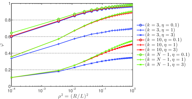
Figure 1: Order parameter $\varphi$ versus square of the normalized metric distance $\rho^{2}=(R/L)^{2}$ in log scale for three different values of $k$: $k=3,\ 10,\ N-1$, and three noise levels: low $\eta=0.1$, medium $\eta=1$, and high $\eta=3$. Each data point is obtained by means of a mixed ensemble averaging of 20 independently-computed dynamics of 500 iteration steps yielding a statistically ample enough sampling.

Up to this point, our analysis of the swarm dynamics was limited to the ideal case of dynamics in the absence of any noise source—stimulus and response noises dusenbery92:_sensor_ecolog . With both a metric and topological distance, it is well known that an increasing level of extraneous noise triggers a second-order phase transition viscek2012 ; komareji13:_resil_contr_dynam_collec_behav . For very low noise levels, a consensus is guaranteed and after a certain transient the swarm is globally aligned. On the contrary, beyond a certain critical noise level no global consensus can be achieved. The consensus level within the swarm is measured by the following order parameter

$$\varphi=\frac{1}{N}\sum\limits^{N}_{j=1}\frac{v_{j}(t)}{v_{0}}=\frac{1}{N}\sum\limits^{N}_{j=1}\exp\left(\textrm{i}\theta_{j}(t)\right),$$ (26)

with $v_{j}$ the velocity of agent $j$ in complex notation. In the particular case of self-propelled particles, the order parameter $\varphi$ represents the alignment of the collective.

At this stage it is worth highlighting that there exists a vast range of models of self-propelled particles reported in the literature, all stemming from the original Vicsek’s model vicsek95:_novel . Our objective here is not to provide an exhaustive list of those models—many of which can be found in the following review viscek2012 —but instead a representative samples of some of the key developments in relation with the present work. Alternative ways of imposing noise have been considered in Ref. gregoire04:_onset_of_collec_and_cohes_motion , and the inclusion of cohesive forces reported in Refs. gregoire03:_movin ; chate08:_model , while also considering the effects of the ambient fluid in Ref. chate08:_model . Pure topological interactions have been reported in Refs. barberis14:_eviden ; komareji13:_resil_contr_dynam_collec_behav ; shang14:_influen , while a topological density invariant rule based on Voronoi neighbors has been considered in Refs. gregoire03:_movin ; gregoire04:_onset_of_collec_and_cohes_motion , with a particular emphasis on metric-free interactions that can be found in Ref. ginelli10:_relev_metric_inter_flock_phenom . Very recently, the effects of limited information flow due to limitations in the bandwidth of the signaling network have been reported in Ref. komareji14:_swarm .

We now turn to the simulations of the dynamics of a swarm of $N=100$ agents initially evenly distributed in a square domain of size $L=\sqrt{N}$ so as to have a unit density as considered in Sec. 2. We intentionally consider the dynamics of small-size swarms as our interest lies in artificial swarms hsieh08:_decen ; naruse13:_veloc_correl_swarm_robtos_direc_neigh and some other natural collectives calovi14:_collec ; attanasi14:_infor with swarmers numbering in the tens to a few hundreds maximum. Given the value of $N$ considered here, some strong small-size effects are expected and in particular, the phase transitions—from a disordered state to collective motion when reducing the ambient noise level—will appear to be continuous (i.e. of second-order type) while they are actually discontinuous (i.e. of first-order type) as proved in several studies chate08:_collec ; chate08:_model ; gregoire04:_onset_of_collec_and_cohes_motion .

For simplicity, we focus on the constant speed case corresponding to $v_{0}=0.1$ that falls into the typical range of values used for such simulations viscek2012 . Noise can generally be assumed to be random fluctuations with a normal distribution dusenbery92:_sensor_ecolog . In the sequel, the background noise is considered to have a normal distribution fully characterized by its noise level, $\eta$. Specifically, starting from the continuous-time equation (1), the presence of noise leads to the following discrete-time equation governing the dynamics of agent $i$:

$$\theta_{i}(t+\Delta t)=\theta_{i}(t)+\frac{\Delta t}{k_{i}}\left[(\theta_{j}(t)-\theta_{i}(t))+\cdots\right.$$

$$\left.+(\theta_{j+k_{i}-1}(t)-\theta_{i}(t))\right]+\Delta\theta_{i},$$ (27)

where $\Delta\theta_{i}$ is a random number chosen with a uniform probability from the interval $[-\eta/2,\ \eta/2]$. The agents positions $\{\mathbf{x}_{i}\}_{i=1,\dots,N}$ are updated according to the discrete-time kinematic rule

$$\mathbf{x}_{i}(t+\Delta t)=\mathbf{x}_{i}(t)+\mathbf{v}_{i}\Delta t,$$ (28)

with $\mathbf{v}_{i}$ having the same definition as previously introduced in Sec. 2. As for the time advance, the canonical value $\Delta t=1$ is considered throughout viscek2012 .The neighborhood of interaction for this swarm model being given by the hybrid metric-topological one, three independent parameters—namely the metric radius $R$, the maximum number of topological neighbors $k$ within the radius $R$ and the noise level $\eta$—influence the emergence of order.

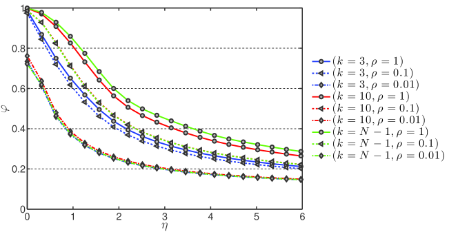
Figure 2: Order parameter $\varphi$ versus noise level $\eta$ for three different values of $k$: $k=3,\ 10,\ N-1$, and three vastly different values of the normalized metric distance: $\rho=R/L=1,\ 0.1,\ 0.01$. Each data point is obtained by means of a mixed ensemble averaging of 20 independently-computed dynamics of 500 iteration steps yielding a statistically ample enough sampling.

Figure 1 displays the variations of the order parameter $\varphi$ with the square of the normalized metric radius $\rho^{2}=(R/L)^{2}$ as hinted from Theorem A. The results gathered in Fig. 1 allow us to draw several interesting comments. First, as expected from the mathematical results in Sec. 2, an increase in the metric radius $R$ systematically yields an increase in the alignment of the swarm for all values of $k$ and of the noise level considered. Second, for any given value of $R$ and for all three noise levels considered, the order parameter is found to increase with $k$ with a dramatic jump in $\varphi$ when $k$ goes from 3 to 10 but with a minute and yet noticeable increase when $k$ goes from 10 to $N-1$. Note that the case $k=N-1$ corresponds to the extreme case of an all-to-all connectivity of the swarm interaction network; in other words each agent interacts with all the others which amounts to what is probably the most cost-ineffective mode of swarming. This case $k=N-1$ also corresponds to a pure metric interaction while the case $\rho=1$ corresponds to the purely topological one. This second result is in complete agreement with the analysis of the influence of the value of $k$ on the consensus reaching dynamics by Shang & Bouffanais shang14:_influen .

To further appreciate the transition between the topological and the metric component of the hybrid interaction distance, one may compare $k$ with the actual number $n^{*}(k)$ of neighbors typically found within the metric disk of radius $R$ centered about the agent. For a given value of the density $\nu=N/L^{2}$ of the swarmers, one finds $n^{*}(k)\simeq\nu\pi R^{2}$. On the one hand, when $k>n^{*}(k)$ it is expected that the topological component becomes ineffective and therefore the hybrid interaction reduces to a purely metric one. Since we investigate the constant density $\nu=1$ case, this situation is bound to happen for small values of $R$, or equivalently $\rho$. On the other hand, when $k<n^{*}(k)$, the topological component takes over the hybrid interaction. This indeed is the case for the largest possible value for $R$, namely $R=L$ or equivalently $\rho=1$. This analysis is consistent with the results shown in Fig. 1 and the related discussion above.

The influence of the noise level is better appreciated when turning to the results reported in Fig. 2. An increase in the noise $\eta$ systematically translates into a reduction of the swarm alignment. As anticipated, the phase transition from an aligned state to a disordered one occurs much earlier for smaller values of $R$. This observation also holds for smaller values of $k$. However, the cases $k=10$ and $k=N-1$ yield extremely close results for not too large values of $R$ and at any given noise level $\eta$. Furthermore, the phase transitions associated with the rapid decay of the order parameter $\varphi$ with noise level $\eta$, for different values of $(k,\rho)$ shown in Fig. 2 are qualitatively consistent with those reported by Barberis & Albano barberis14:_eviden . Note that the comparison can only be qualitative owing to the fact that the time update rule used in Ref. barberis14:_eviden is slightly different from the one considered in the present study, namely Eq. (27). The exact same comment also applies to the comparison of our results gathered in Fig. 2 with those obtained by Niizato & Gunji niizato11:_metric with yet another time update rule and another framework for their hybrid metric-topological interaction distance.

4 Conclusions

A combined computational and theoretical analysis of the dynamics of swarms of self-propelled agents subjected to a hybrid metric-topological neighborhood of interaction has been performed. The hybrid interaction distance is devised to overcome fundamental issues associated with inherent limitations in the sensory range and information-processing capabilities encountered in real-life natural and artificial complex systems. The results reported in this article allow us to formulate the following important conclusions:

• When the agent density in the field is constant (here the unity), the consensus dynamics is exclusively dominated by the metric component $R$ of our hybrid model. As long as $k\geq 1$, one can always observe the emergence of consensus with some positive probability in the absence of noise. This result is further extended to the case of agents having non-constant speeds.

• For large swarms and still in the absence of noise, the probability of emergence of consensus is approximately proportional to $R^{2}$.

• Similarly to swarms subjected to a purely metric or a purely topological distance, a collapse of the swarm alignment is observed in the presence of a sufficiently-high noise level using our hybrid model. Furthermore, our results confirm the ineffectiveness of the purely metric model which yields a marginally higher alignment at the expense of a very large number of social interactions as compared to the case $k=10$ shang14:_influen .

Furthermore, our initial observations reveal that the number of topological neighbors $k$ solely affects the speed with which consensus is reached as observed in the purely topological distance case shang14:_influen . However, this last point requires a more thorough investigation to provide a clear picture of the consensus reaching dynamics for a swarm ruled by a hybrid interaction distance.

5 Acknowledgments

We thank Dr. Mohammad Komareji for fruitful and stimulating conversations.

This work was supported by a grant from the SUTD-MIT International Design Centre (RB) and a grant by the Temasek Lab (TL$@$SUTD) under the STARS project (YS & RB).

References

- (1) S. Camazine, J.-L. Deneubourg, N. R. Franks, J. Sneyd, G. Theraulaz, and E. Bonabeau. Self-Organization in Biological Systems. Princeton University Press, Princeton, New Jersey, 2001.
- (2) R. Bouffanais. Design and Control of Swarm Dynamics. Springer, Complexity Series, Singapore, 2016.
- (3) T. Vicsek and A. Zafeiris. Collective motion. Phys. Rep., 517:71–140, 2012.
- (4) R. Bouffanais and D. K. P. Yue. Hydrodynamics of cell-cell mechanical signaling in the initial stages of aggregation. Phys. Rev. E, 81:041920, 2010.
- (5) D. J. T. Sumpter. The principles of collective animal behaviour. Phil. Trans. R. Soc. B, 361:5–22, 2006.
- (6) D. J. T. Sumpter. Collective Animal Behavior. Princeton University Press, Princeton, NJ, 2010.
- (7) M. Ani Hsieh, Vijay Kumar, and Luiz Chaimowicz. Decentralized controllers for shape generation with robotic swarms. Robotica, 26:691–701, 8 2008.
- (8) Keitaro Naruse. Velocity correlation in swarm robots with directional neighborhood. In S. Lee, H.S. Cho, K.J. Yoon, and J.M. (Eds.) Lee, editors, Intelligent Autonomous Systems 12, pages 843–851. Advances in Intelligent Systems and Computing, 2013.
- (9) C. K. Hemelrijk and H. Hildenbrandt. Self-organised shape and frontal density of fish schools. Ethology, 114:245–254, 2008.
- (10) C. K. Hemelrijk and H. Hildenbrandt. Schools of fish and flocks of birds: Their shape and internal structure by self-organization. Interface Focus, 2:726–737, 2012.
- (11) C. K. Hemelrijk and H. Hildenbrandt. Some causes of the variable shape of flocks of birds. PLoS one, 6:e22479, 2011.
- (12) M. Ballerini, N. Cabibbo, R. Candelier, A. Cavagna, E. Cisbani, I. Giardina, V. Lecomte, A. Orlandi, G. Parisi, A. Procaccini, M. Viale, and V. Zdravkovic. Interaction ruling animal collective behavior depends on topological rather than metric distance: Evidence from a field study. Proc. Natl. Acad. Sci. USA, 105:1232–1237, 2008.
- (13) F. Ginelli and H. Chaté. Relevance of metric-free interactions in flocking phenomena. Phys. Rev. Lett., 105:168103, 2010.
- (14) M. Moussaïd, D. Helbing, and G. Theraulaz. How simple rules determine pedestrian behavior and crowd disasters. Proc. Natl. Acad. Sci. USA, 108:6884–6888, 2011.
- (15) S. Coombs and J. C. Montgomery. The enigmatic lateral line system. In R. R. Fay and A. N. Popper, editors, Comparative Hearing: Fish and Amphibians, Springer Handbook of Auditory Research, pages 319–362. Springer-Verlag, New York, 1999.
- (16) R. Bouffanais, G. D. Weymouth, and D. K. P. Yue. Hydrodynamic object recognition using pressure sensing. Proc. R. Soc. A, 467:19–38, 2011.
- (17) David B. Dusenbery. Sensory Ecology: How organisms acquire and respond to information. W. H. Freeman and Co., New York, 1992.
- (18) J. Emmerton and J. Delius. Vision, Brain, and Behavior in Birds, chapter Beyond sensation: Visual cognition in pigeons, pages 377–390. MIT Press, Cambridge MA, Zeigler, H. and Bischof, H.J. edition, 1993.
- (19) T. Niizato and Y.-P. Gunji. Metric-topological interaction model of collective behavior. Ecol. Model., 222:3041–3049, 2011.
- (20) L. Barberis and E. V. Albano. Evidence of a robust universality class in the critical behavior of self-propelled agents: Metric versus topological interactions. Phys. Rev. E, 89:012139, 2014.
- (21) H. G. Tanner, A. Jadbabaie, and J. P. Pappas. Stable flocking of mobile agents, part i: Fixed topology. In Proc. of the 42nd IEEE Conference on Decision and Control, pages 2010–2015, Maui, Hawaii USA, 2003. IEEE.
- (22) H. G. Tanner, A. Jadbabaie, and J. P. Pappas. Flocking in fixed and switching networks. IEEE Trans. Automat. Control, 52:863–868, 2007.
- (23) M. Komareji and R. Bouffanais. Resilience and controllability of dynamic collective behaviors. PLoS One, 8:e82578, 2013.
- (24) Y. Shang and R. Bouffanais. Influence of the number of topologically interacting neighbors on swarm dynamics. Sci. Rep., 4:4184, 2014.
- (25) P. Miller. The Smart Swarm. Penguin Group, 2010.
- (26) M. Aldana, V. Dossetti, C. Huepe, V. M. Kenkre, and H. Larralde. Phase transitions in systems of self-propelled agents and related network models. Phys. Rev. Lett., 98:095702, 2007.
- (27) R. Olfati-Saber, J. A. Fax, and R. M. Murray. Consensus and cooperation in networked multi-agent systems. Proc. IEEE, 95(1):215–233, 2007.
- (28) D. Eppstein, M. S. Paterson, and F. F. Yao. On nearest-neighbor graphs. Discrete and Computational Geometry, 17:263–282, 1997.
- (29) P. Balister, B. Bollobás, A. Sarkar, and M. Walters. Connectivity of random -nearest neighbour graphs. Adv. Appl. Probab., 37:1–24, 2005.
- (30) P. Balister, B. Bollobás, A. Sarkar, and M. Walters. A critical constant for the -nearest neighbour model. Adv. Appl. Probab., 41:1–12, 2009.
- (31) W. Ren and R.W. Beard. Consensus seeking in multiagent systems under dynamically changing interaction topologies. IEEE Trans. Autom. Control, 50:655–661, 2005.
- (32) H. Chaté, F. Ginelli, G. Grégoire, F. Peruani, and F. Raynaud. Modeling collective motion: variations on the vicsek model. Eur. Phys. J. B, 64:451–456, 2008.
- (33) G. Grégoire, H. Chaté, and Y. H. Tu. Moving and staying together without a leader. Physica D-nonlinear Phenomena, 181:157–170, 2003.
- (34) G. Grégoire and H. Chaté. Onset of collective and cohesive motion. Phys. Rev. Lett., 92:025702, 2004.
- (35) I. Matei, J. Baras, and C. Somarakis. Convergence results for the linear consensus problem under markovian random graphs. SIAM J. Control Optim., 51:1574–1591, 2013.
- (36) I. Matei, N. Martins, and J. Baras. Almost sure convergence to consensus in Markovian random graphs. In Proc. of the 47th IEEE Conference on Decision and Control, pages 3535––3540, Cancún, Mexico, 2008.
- (37) M. Huang, S. Dey, G. N. Nair, and J. H. Manton. Stochastic consensus over noisy networks with Markovian and arbitrary switches. Automotica, 46:1571–1583, 2010.
- (38) T. Vicsek, A. Czirók, E. Ben-Jacob, I. Cohen, and O. Shochet. Novel type of phase-transition in a system of self-driven particles. Phys. Rev. Lett., 75:1226–1229, 1995.
- (39) M. Komareji, Y. Shang, and R. Bouffanais. Swarming collapse under limited information flow between individuals. arXiv:1409.7207, September 2014.
- (40) D. S. Calovi, U. Lopez, P. Schuhmacher, H. Chaté, C. Sire, and G. Theraulaz. Collective response to perturbations in a data-driven fish school model. arXiv:1409.6430, September 2014.
- (41) A. Attanasi, A. Cavagna, L. Del Castello, I. Giardina, T. S. Grigera, A. Jelić, S. Melillo, L. Parisi, O. Pohl, E. Shen, and M. Viale. Information transfer and behavioural inertia in starling flocks. Nature Phys., 10:691–696, 2014.
- (42) H. Chaté, F. Ginelli, G. Grégoire, and F. Raynaud. Collective motion of self-propelled particles interacting without cohesion. Phys. Rev. E, 77:046113, 2008.