Range-separated meta-GGA functional designed for noncovalent interactions

Abstract

The accuracy of applying density functional theory to noncovalent interactions is hindered by errors arising from low-density regions of interaction-induced change in the density gradient, error compensation between correlation and exchange functionals, and dispersion double counting. A new exchange-correlation functional designed for noncovalent interactions is proposed to address these problems. The functional consists of the range-separated PBEsol exchange considered in two variants, pure and hybrid, and the semilocal correlation functional of Modrzejewski et al. [J. Chem. Phys. 137, 204121 (2012)] designed with the constraint satisfaction technique to smoothly connect with a dispersion term. Two variants of dispersion correction are appended to the correlation functional: the atom-atom pairwise additive DFT-D3 model and the density-dependent many-body dispersion with self-consistent screening (MBD-rsSCS). From these building blocks a set of four functionals is created to systematically examine the role of pure versus hybrid exchange and the underlying models for dispersion. The new functional is extensively tested on benchmark sets with diverse nature and size. The truly outstanding performance is demonstrated for water clusters of varying size, ionic hydrogen bonds, and thermochemistry of isodesmic n-alkane fragmentation reactions. The merits of each component of the new functional are discussed.

I Introduction

DFT is one of few quantum-chemical methods capable of dealing with problems germane to molecular biology and materials science which involve electronic structure, yet on a scale too large for ab initio wavefunction tools. So far, however, the approximate character of affordable functionals seriously restricts their predictive power in several important areas, the most prominent ones being related to noncovalently bound systems. An approximate functional focused on performance for noncovalent interactions is the subject of this work.

During the past decade, a large effort has been devoted to resolve the deficiencies in the description of noncovalent interactions. The progress has been indicated by steady improvement of statistical errors in databases of noncovalent interactions.Burns et al. (2011); Podeszwa and Szalewicz (2012) Still, part of this apparent advancement is a result of error cancellation between the dispersion-free part of a functional and its a posteriori dispersion correction. Consequently, even for the best performing methods, there exist systems for which the cancellation does not occur and error spikes beyond the average levels. Examples of such problematic systems are water clusters studied in this work.

A practical chemist copes with the issue of large, unpredictable errors by cross-checking her calculations with several independent approximate functionals. Thus, to make DFT a dependable tool, we still need new functionals developed independently from the currently existing ones and built from well-defined components, which do not exploit obscure error cancellation.

This work introduces a set of new DFT exchange-correlation functionals intended primarily for noncovalent interactions. They are composed of the recent meta-GGA correlation developed by Modrzejewski et al. (2012), the range-separated PBEsol exchangePerdew et al. (2008); Csonka et al. (2008); Henderson, Janesko, and Scuseria (2008) ($\omega$PBEsol), and a dispersion correction,

$$E_{\mathrm{XC}}=E_{\mathrm{C}}+E_{\mathrm{X}}(\omega\text{PBEsol})+E_{\mathrm{disp}}.$$ (1)

The two variants of the dispersion correction employed in this work are DFT-D3 by Grimme et al. (2010) (abbreviated as D3) and MBD-rsSCS by Ambrosetti et al. (2014) (abbreviated as MBD). There are other possible ways of including dispersion not explored here.Lee et al. (2010); Vydrov and Van Voorhis (2010); Sato and Nakai (2010); Becke and Johnson (2005) Furthermore, we assess two variants of short-range exchange: pure PBEsol and a hybrid with an addition of the short-range HF exchange. For brevity, the full exchange will be called either pure or hybrid depending on the fraction of the short-range exact exchange. In total, there are four combinations of the exchange and dispersion components: MCS-D3, MCS-MBD, MCSh-D3, and MCSh-MBD, where the first part of the label denotes the exchange approximation (MCS for the pure exchange and MCSh for the hybrid) and the second part specifies the dispersion correction. This set of functionals will be collectively referred to as MCS.

The MCS functionals are designed to overcome several issues of the currently available exchange-correlation approximations.

First, a part of the difficulties in the description of noncovalent systems can be pinpointed to the poor behavior of approximate exchange functionals in the low-density regions where the density gradient changes substantially upon bond formation.Lacks and Gordon (1993); Murray, Lee, and Langreth (2009) The emergence of such regions is the signature of noncovalent bondingJohnson et al. (2010) and is the source of major contributions to the interaction energy.Lacks and Gordon (1993); Murray, Lee, and Langreth (2009) For example, depending on the limit of an exchange enhancement factor for large reduced gradients, the exchange-only interaction curve of a noble gas dimer can be either attractive (as in PBE) or much more repulsive than the Hartree-Fock limit (as in B88).Kannemann and Becke (2009) Although the behavior of the exchange is not decisive for the performance of the full exchange-correlation functional due to the possible error cancellation, it may obscure the interpretation of interaction energies and eventually worsen the compatibility with dispersion corrections. One way of ensuring that DFT exchange-only interaction curves resemble the Hartree-Fock ones is by employing range-separated exchange functionals.Kamiya, Tsuneda, and Hirao (2002) Also inclusion of the exact second-order gradient expansion of the exchange functional improves description of the regions relevant for noncovalent systems.Csonka et al. (2008); Johnson, Contreras-García, and Yang (2012) The $\omega$PBEsol exchange included in the MCS functionals combines both of these remedies.

The second problem with the existing DFT treatments of noncovalent interactions is that a dispersion correction, such as D3, tends to disguise the shortcomings of the base semilocal functional. This may lead to an inconsistency that the long-range dispersion correction calibrated for an underbinding semilocal functional becomes larger than the reference value of the total dispersion as obtained from the SAPT approach.Misquitta et al. (2005) A BLYP-D3 treatment of complexes from the S22 database serves as an example of such an inconsistency. We discuss this issue later in the text.

The third possible source of errors is double counting of short-range correlation by a semilocal correlation functional and a dispersion correction. The semilocal correlation model employed here is designed to avoid this issue via the design of the corresponding correlation hole. The hole is equipped with a single empirical parameter to control its range. To eliminate the overlap with the dispersion correction, the damping of the hole for large $r_{12}$ is adjusted through empirical optimization.Modrzejewski et al. (2012)

Some of the features of a density functional deemed here important for noncovalent systems have been recognized and built into the $\omega$B97X-DChai and Head-Gordon (2008) and $\omega$B97X-D3Lin et al. (2013) functionals. Both of these models employ range-separated exchange and have $15$ empirical parameters in their energy expressions optimized simultaneously with the dispersion corrections. (A systematic analysis of the B97-type functionals has demonstrated, however, that the number of empirical parameters should be reduced to improve the performance outside the training sets.Mardirossian and Head-Gordon (2014)) The dispersionless density functional of Pernal et al. (2009) is also an example of a heavily parametrized functional designed to be used in combination with a dispersion term.

II Theory

II.1 Semilocal correlation

The first term of Eq. 1, $E_{\mathrm{C}}$, stands for the recently proposed correlation functional of Modrzejewski et al. (2012) The functional has been derived starting from a meta-GGA model for the spin-resolved correlation hole,

$$h_{\mathrm{C}\lambda}^{\alpha\beta}(\mathbf{r}_{1},r_{12}) =(a_{\alpha\beta}+b_{\alpha\beta}r_{12}+c_{\alpha\beta}r_{12}^{2})\exp(-d_{\alpha\beta}r_{12}),$$ (2)

$$h_{\mathrm{C}\lambda}^{\alpha\alpha}(\mathbf{r}_{1},r_{12}) =r_{12}^{2}(a_{\alpha\alpha}+b_{\alpha\alpha}r_{12}+c_{\alpha\alpha}r_{12}^{2})\exp(-d_{\alpha\alpha}r_{12}),$$ (3)

where $a_{\sigma\sigma^{\prime}}$, $b_{\sigma\sigma^{\prime}}$, and $c_{\sigma\sigma^{\prime}}$ are functions of density at a given point, obtained from analytic formulas for the short-range (small $r_{12}$) part of the pair correlation function in the homogeneous electron gas.Gori-Giorgi and Perdew (2001); Rassolov, Pople, and Ratner (2000) These formulas were modified to include dependence on the kinetic energy density to eliminate the spurious self-interaction in the parallel-spin part.Modrzejewski et al. (2012) The only empirical parameter of the correlation model, $G$, governs the exponential damping,

$$d_{\alpha\beta} =\frac{2.1070}{r_{\mathrm{s}}^{\alpha\beta}}+d_{\mathrm{grad}},$$ (4)

$$d_{\alpha\alpha} =\frac{2.6422}{r_{\mathrm{s}}^{\alpha\alpha}}+d_{\mathrm{grad}},$$ (5)

$$d_{\mathrm{grad}} =\frac{G}{r_{\mathrm{s}}}\frac{\nabla\rho\cdot\nabla\rho}{\rho^{8/3}}.$$ (6)

The larger the numerical value of $G$, the more short-ranged character of $h_{\mathrm{C}\lambda}^{\sigma\sigma^{\prime}}(\mathbf{r}_{1},r_{12})$. Thus, $G$ can be optimized to adjust the range of the approximate correlation hole to complement, in the manner that avoids double counting, the long-range correlation contributed by the selected variant of a dispersion correction. It should be emphasized that all the exact constraints that are built into our correlation model are obeyed when varying the value of $G$.Modrzejewski et al. (2012) In particular, the short-range Taylor expansion of $h_{\mathrm{C}\lambda}^{\sigma\sigma^{\prime}}(\mathbf{r}_{1},r_{12})$, which has been accurately modeled after the homogeneous electron gas,Gori-Giorgi and Perdew (2001) remains unchanged when tuning the correlation functional to a specific dispersion correction and an exchange functional. Put differently, the empirical adjustment applied to merge the long-range dispersion with the semilocal correlation does not adversely affect the features which are reliable already at the semilocal level.Burke, Perdew, and Ernzerhof (1998)

For reader’s convenience, we present $E_{\mathrm{C}}$ in a form ready for implementation. Following Ref. 3, $E_{\mathrm{C}}$ is represented as a sum of spin-parallel and antiparallel components:

$$E_{\mathrm{C}}=E_{\mathrm{C}}^{\alpha\beta}+E_{\mathrm{C}}^{\beta\alpha}+E_{\mathrm{C}}^{\alpha\alpha}+E_{\mathrm{C}}^{\beta\beta}.$$ (7)

As for any semilocal functional, $E_{\mathrm{C}}$ is evaluated by numerically integrating the density of the correlation energy on a molecular grid,

$$E_{\mathrm{C}}^{\alpha\beta} =\frac{1}{2}\int\mathrm{d}^{3}\mathbf{r}_{1}\int_{0}^{1}\mathrm{d}\lambda\int_{0}^{\infty}\frac{\rho_{\alpha}(\mathbf{r}_{1})h_{\mathrm{C}\lambda}^{\alpha\beta}(\mathbf{r}_{1},r_{12})}{r_{12}}4\pi r_{12}^{2}\mathrm{d}r_{12}$$

$$=\int\mathrm{d}^{3}\mathbf{r}_{1}\rho_{\alpha}\pi\frac{\mathcal{B}_{\alpha\beta}+\mathcal{A}_{\alpha\beta}d_{\alpha\beta}}{d_{\alpha\beta}^{3}},$$ (8)

$$E_{\mathrm{C}}^{\alpha\alpha} =\frac{1}{2}\int\mathrm{d}^{3}\mathbf{r}_{1}\int_{0}^{1}\mathrm{d}\lambda\int_{0}^{\infty}\frac{\rho_{\alpha}(\mathbf{r}_{1})h_{\mathrm{C}\lambda}^{\alpha\alpha}(\mathbf{r}_{1},r_{12})}{r_{12}}4\pi r_{12}^{2}\mathrm{d}r_{12}$$

$$=\int\mathrm{d}^{3}\mathbf{r}_{1}\rho_{\alpha}\pi\frac{8\mathcal{B}_{\alpha\alpha}+4\mathcal{A}_{\alpha\alpha}d_{\alpha\alpha}}{d_{\alpha\alpha}^{5}}.$$ (9)

The integral over the coupling constant $\lambda$ is done analytically. $\mathcal{A}_{\alpha\beta}$, $\mathcal{B}_{\alpha\beta}$, $\mathcal{A}_{\alpha\alpha}$, $\mathcal{B}_{\alpha\alpha}$, $d_{\alpha\beta}$, and $d_{\alpha\alpha}$ are functions evaluated at each grid point,

$$\mathcal{A}_{\alpha\beta} =\frac{\rho_{\beta}}{r_{\mathrm{s}}^{\alpha\beta}}\left[\left(-P_{0}+\sum_{k=1}^{4}P_{k}(r_{\mathrm{s}}^{\alpha\beta})^{k}\right)\exp\left(-P_{5}r_{\mathrm{s}}^{\alpha\beta}\right)+P_{0}\right]-\rho_{\beta},$$ (10)

$$\mathcal{B}_{\alpha\beta} =\frac{\rho_{\beta}}{(r_{\mathrm{s}}^{\alpha\beta})^{2}}\left[\left(-Q_{0}+\sum_{k=1}^{5}Q_{k}(r_{\mathrm{s}}^{\alpha\beta})^{k}\right)\exp\left(-Q_{6}r_{\mathrm{s}}^{\alpha\beta}\right)+Q_{0}\right]+d_{\alpha\beta}\mathcal{A}_{\alpha\beta},$$ (11)

$$\mathcal{A}_{\alpha\alpha} =\frac{D_{\alpha}}{3r_{\mathrm{s}}^{\alpha\alpha}}\left[\left(-R_{0}+\sum_{k=1}^{2}R_{k}(r_{\mathrm{s}}^{\alpha\alpha})^{k}\right)\exp\left(-R_{3}r_{\mathrm{s}}^{\alpha\alpha}\right)+R_{0}\right]-\frac{D_{\alpha}}{3},$$ (12)

$$\mathcal{B}_{\alpha\alpha} =\frac{D_{\alpha}}{6(r_{\mathrm{s}}^{\alpha\alpha})^{2}}\left[\left(-S_{0}+\sum_{k=1}^{3}S_{k}(r_{\mathrm{s}}^{\alpha\alpha})^{k}\right)\exp\left(-S_{4}r_{\mathrm{s}}^{\alpha\alpha}\right)+S_{0}\right]+d_{\alpha\alpha}\mathcal{A}_{\alpha\alpha}.$$ (13)

The symbols in Eqs. 4-6 and Eqs. 8-13 are defined as follows: $\rho_{\alpha}$ and $\rho_{\beta}$ are electronic spin-densities; $\rho$ is the total electronic density; $\tau_{\alpha}$ is the kinetic energy density,

$$\tau_{\alpha}=\sum_{i}^{N_{\alpha}}|\nabla\psi_{i\alpha}|^{2};$$ (14)

the variable $D_{\alpha}$ appearing in the parallel-spin part depends on the electron density, its gradient, and $\tau_{\alpha}$,

$$D_{\alpha}=\tau_{\alpha}-\frac{|\nabla\rho_{\alpha}|^{2}}{4\rho_{\alpha}};$$ (15)

$r_{\mathrm{s}}^{\alpha\alpha}$, $r_{\mathrm{s}}^{\alpha\beta}$, and $r_{\mathrm{s}}$ depend only on electron (spin)-densities:

$$r_{\mathrm{s}}^{\alpha\alpha} =\frac{\left(3/\pi\right)^{1/3}}{2\rho_{\alpha}^{1/3}},$$ (16)

$$r_{\mathrm{s}}^{\alpha\beta} =\frac{\left(3/\pi\right)^{1/3}}{\rho_{\alpha}^{1/3}+\rho_{\beta}^{1/3}},$$ (17)

$$r_{\mathrm{s}} =\left(\frac{3}{4\pi\rho}\right)^{1/3}.$$ (18)

$E_{\mathrm{C}}^{\beta\beta}$ is obtained by relabeling the spin indices in $E_{\mathrm{C}}^{\alpha\alpha}$; note also that the equality $E_{\mathrm{C}}^{\alpha\beta}=E_{\mathrm{C}}^{\beta\alpha}$ holds. The only empirical parameter in the correlation functional is $G$ (see Table 2). The nonempirical parameters appearing in Eqs. 10-13 are derived from a short-range model of the correlation hole in the homogeneous electron gas.Modrzejewski et al. (2012) Their values are defined in Table 1.

Table 1: Ab initio numerical constants appearing in Eqs. 10–13.

k	$P_{k}$	$Q_{k}$	$R_{k}$	$S_{k}$
$0$	$1.696$	$3.356$	$1.775$	$3.205$
$1$	$-0.2763$	$-2.525$	$0.01213$	$-1.784$
$2$	$-0.09359$	$-0.4500$	$-4.743\times 10^{-3}$	$3.613\times 10^{-3}$
$3$	$3.837\times 10^{-3}$	$-0.1060$	$0.5566$	$-4.743\times 10^{-3}$
$4$	$-2.471\times 10^{-3}$	$5.532\times 10^{-4}$		$0.5566$
$5$	$0.7524$	$-2.471\times 10^{-3}$
$6$		$0.7524$

Table 2: Empirical parameters of the four tested MCS functionals. The columns labeled “MCS” and “MCSh” correspond to the pure and hybrid variants of the exchange, respectively.

name	MCS	MCSh	definition
$G$	0.075	0.100	Eq. 6
$\omega$	0.300	0.200	Eq. 24
$\alpha$	0.000	0.200	Eq. 23
D3 dispersion
$r_{6}$	1.1822	1.2900	Eq. 20
$s_{8}$	0.7740	1.3996	Eq. 19
MBD dispersion
$\beta$	0.8033	0.7242	Eq. 22

II.2 Dispersion correction

The semilocal exchange-correlation functional is supplemented with a dispersion correction. To confirm the versatility of our approach, we assess two models of the dispersion interaction: D3Grimme et al. (2010) and MBD.Ambrosetti et al. (2014)

The dispersion energy in the D3 approximation is defined as

$$E_{\mathrm{disp}}(\text{D3}) =\sum_{AB}\sum_{n=6,8}s_{n}\frac{C^{AB}_{n}}{R^{n}_{AB}}f_{n}\left(R_{AB}\right),$$ (19)

$$f_{n}\left(R_{AB}\right) =\frac{1}{1+6(R_{AB}/(r_{n}R^{AB}_{0}))^{-\alpha_{n}}}.$$ (20)

The D3 model contains two empirical, functional-dependent parameters:Grimme et al. (2010) $s_{8}$ and $r_{6}$. Other parameters appearing in Eqs. 19 and 20 are common to all functionals and are defined in Ref. 7. The $C_{6}^{AB}$ coefficients are interpolated from the ab initio tabulated data obtained for hydrides.Grimme et al. (2010) The main advantage of D3 is that it is thoroughly testedBurns et al. (2011) and available in almost any quantum-chemical program. It also offers simple to compute derivatives with respect to nuclear coordinates, which is important for structure optimizations.

The second considered model of the dispersion interaction is MBD.Ambrosetti et al. (2014) A computation of the MBD energy requires two steps. First, the screening equationTkatchenko et al. (2012) is solved for frequency-dependent polarizabilities. Then, the solution of the screening equation is used to set up the Hamiltonian of interacting quantum harmonic oscillators whose correlation energy models the long-range dispersion energy of the real system. While the computational cost of MBD is larger than that of D3, it is still negligible compared to the SCF step. The dipole interaction in the screening equation as well as in the MBD Hamiltonian is range separated with a Fermi-type damping function:Ambrosetti et al. (2014)

$$f_{\mathrm{MBD}}(R_{AB}) =\frac{1}{1+\exp\left[-6\left(R_{AB}/S_{\mathrm{vdW}}-1\right)\right]},$$ (21)

$$S_{\mathrm{vdW}} =\beta(R_{\mathrm{vdW}}^{A}+R_{\mathrm{vdW}}^{B}),$$ (22)

where $\beta$ is the only functional-dependent parameter of the model. The MBD model is expected to be a good approximation for large molecular systems where an atom-pairwise approximation may no longer capture the many-body contributions to the total interaction energy.Ruzsinszky et al. (2012); Gobre and Tkatchenko (2013)

II.3 Exchange

The exchange functional is composed of the short-range $\omega$PBEsol exchange,Henderson, Janesko, and Scuseria (2008) long-range HF exchange, and optionally a fraction $\alpha$ of the short-range HF exchange,

$$E_{\mathrm{X,SR}}=(1-\alpha)E_{\mathrm{X,SR}}(\omega\mathrm{PBEsol})+\alpha E_{\mathrm{X,SR}}(\mathrm{HF}).$$ (23)

The short-range and long-range parts of $E_{\mathrm{X}}$ are defined through the decomposition of the $1/r_{12}$ operator,

$$\frac{1}{r_{12}}=\frac{\mathrm{erfc}\left(\omega r_{12}\right)}{r_{12}}+\frac{\mathrm{erf}\left(\omega r_{12}\right)}{r_{12}}.$$ (24)

We test two variants of the exchange functional: pure ($\alpha=0$ and $\omega=0.3$) and hybrid ($\alpha=0.2$ and $\omega=0.2$). The range separation parameter $\omega$ for the pure variant is obtained via empirical optimization. The parameters $\alpha$ and $\omega$ of the hybrid variant are assumed the same as for the LRC-$\omega$PBEh functional of Rohrdanz, Martins, and Herbert (2009) It is worthwhile to note that whereas the fixed value of $\omega$ is convenient in practical computations, the optimal $\omega$ depends on the system size and electronic structure, which is especially important for donor-acceptor systems.Modrzejewski et al. (2013); Koppen et al. (2014)

The PBEsol exchange,Perdew et al. (2008) which is the basis for $\omega$PBEsol, has the exact second-order gradient expansion. This feature is important for solidsPerdew et al. (2008) and for large organic molecules.Csonka et al. (2008) In contrast to PBEsol, the gradient expansion of the PBE exchange is not exact; it is designed to cancel the gradient term of the PBE correlation,Csonka et al. (2008) which makes it less suitable than PBEsol in conjunction with our correlation functional.

III Technical details

The functionals employed in this study, besides the MCS functionals, are $\omega$PBE,Perdew, Burke, and Ernzerhof (1996); Henderson, Janesko, and Scuseria (2008) B3LYP,Stephens et al. (1994) BLYP,Gill et al. (1992) M06,Zhao and Truhlar (2008) M06-2X,Zhao and Truhlar (2008) and $\omega$B97X-D.Chai and Head-Gordon (2008) $\omega$PBE has its range separation parameter fixed at $\omega=0.4$. The suffix “-D3” denotes functionals with added Grimme’s D3 correction.Grimme et al. (2010) For water 16-mers and for the S22 database the energies are obtained with the LC-$\omega$PBE functionalVydrov et al. (2006) instead of $\omega$PBE. We supply $\omega$PBE and LC-$\omega$PBE with the same D3 correction calibrated by Grimme et al. (2010) All DFT computations employ the def2-TZVPPD basisWeigend and Ahlrichs (2005); Schuchardt et al. (2007) unless noted otherwise. The acronyms used to name the types of errors are: mean-absolute percentage deviation (MAPD), root-mean-square deviation (RMSD), mean absolute deviation (MAD), and mean signed deviation (MSD). Energies are given in kcal/mol.

The training set for the MCS-D3 and MCSh-D3 functionals is composed of the noncovalent interactions database of Zhao and Truhlar.Zhao and Truhlar (2005a, b) The training database is partitioned into subsets according to the nature of the represented interactions. The subsets are as follows: WI7/05 (small, dispersion-dominated complexes), PPS5/05 ($\pi$-electron dispersion interactions), DI6-04 (dispersion and dipole interactions), HB6/04 (hydrogen bonds), and CT7/04 (ground-state charge-transfer interactions).

The optimization of the MCS-D3 functional consisted of the following steps. First, we generated a grid of parameters $(\omega,G)$ satisfying $0.100\leq\omega\leq 0.450$ and $0.050\leq G\leq 0.150$; for each pair $(\omega,G)$, we optimized the D3 correction by finding the pair $(r_{6},s_{8})$ which minimized the objective function

$$F(r_{6},s_{8};\omega,G)=10\times\text{RMSD(WI7/05)}+\text{RMSD(other)},$$ (25)

where RMSD(X) denotes the root-mean-square deviation within the subset X of the training set. Finally, we selected the parameters $(\omega,G,r_{6},s_{8})$ corresponding the smallest MAD and MAPD. Table 3 presents the results for the training set.

For the MCS-MBD functional we kept the same values of $\omega$ and $G$ as for MCS-D3. The only difference is that the parameter $\beta$ of the MBD dispersion was obtained by minimization of RMSD for the S22 set.Jurecka et al. (2006) The different choice of the training sets for the D3 and MBD corrections was due to the poor behavior of the latter for small dispersion-bound dimers.

For the hybrid MCS functionals, MCSh-D3 and MCSh-MBD, we did not optimize $\alpha$ and $\omega$, but fixed these parameters at the same values as in the LRC-$\omega$PBEh functional.Rohrdanz, Martins, and Herbert (2009) The parameter $G$ in the semilocal correlation and the dispersion corrections were optimized in the same way as for MCS-D3 and MCS-MBD.

Table 3: Training database for the MCS-D3 and MCSh-D3 functionals. The interaction energies are grouped into five subsets: WI7/05, DI6/04, CT7/04, HB6/04, and PPS5/05. The reference CCSD(T) energies are taken from Ref. 23. The monomer geometries are held rigid at their dimer values. The units are kcal/mol.

Dimer	CCSD(T)	MCS-D3	MCSh-D3
He … Ne	-0.041	-0.020	-0.033
He … Ar	-0.058	-0.016	-0.034
Ne … Ne	-0.086	-0.015	-0.048
Ne … Ar	-0.131	-0.039	-0.061
CH4 … Ne	-0.18	-0.18	-0.18
C6H6 … Ne	-0.41	-0.41	-0.52
CH4 … CH4	-0.53	-0.55	-0.47
H2S … H2S	-1.62	-1.40	-1.52
HCl … HCl	-1.91	-1.54	-1.68
HCl … H2S	-3.26	-3.18	-3.32
CH3Cl … HCl	-3.39	-3.08	-3.26
CH3SH … HCN	-3.58	-3.54	-3.70
CH3SH … HCl	-4.74	-4.94	-5.13
C2H4 … F2	-1.06	-0.98	-1.06
NH3 … F2	-1.80	-1.93	-1.95
C2H2 … ClF	-3.79	-3.74	-3.93
HCN … ClF	-4.80	-4.15	-4.03
NH3 … Cl2	-4.85	-4.86	-5.07
H2O … ClF	-5.20	-5.12	-5.10
NH3 … ClF	-11.17	-13.65	-13.89
NH3 … NH3	-3.09	-2.78	-2.77
HF … HF	-4.49	-4.06	-4.13
H2O … H2O	-4.91	-4.60	-4.61
NH3 … H2O	-6.38	-6.35	-6.29
(HCONH2)2	-15.41	-15.02	-15.14
(HCOOH)2	-17.60	-18.10	-17.94
(C2H2)2	-1.36	-1.24	-1.29
(C2H4)2	-1.44	-1.59	-1.54
sandwich (C6H6)2	-1.65	-1.58	-1.51
T-shaped (C6H6)2	-2.63	-2.79	-2.86
displaced (C6H6)2	-2.59	-2.80	-2.49

To determine the stabilization energy upon complex formation, two definitions are employed: the interaction energy and the binding energy. The interaction energy is defined as

$$E_{\mathrm{int}}=E\left(\text{dimer AB}\right)-E\left(\text{isolated A}\right)-E\left(\text{isolated B}\right),$$ (26)

where the monomer geometries are held rigid at their dimer values, and the counterpoise correction is employed. In the case of water clusters, we use the binding energy instead of $E_{\mathrm{int}}$,

$$E_{\mathrm{bind}}=E\left(\ce{(H2O)_{n}}\right)-nE\left(\ce{(H2O)_{isolated}}\right),$$ (27)

where the coordinates of water molecules relax upon dissociation from the cluster. $E_{\mathrm{bind}}$ does not include the energy of zero-point vibrations. The basis set employed for the isolated H2O monomers does not include any functions centered on the ghost centers.

The reference binding energies of water 16-mers were obtained by combining $\Delta E_{\mathrm{CCSD(T)}}$ with the extrapolated binding energies at the MP2 level, as proposed by Rezac, Riley, and Hobza (2011),

$$E_{\mathrm{bind,CCSD(T)}}^{CBS(AVTZ\rightarrow AVQZ)}=E_{\mathrm{HF}}^{AVQZ}+E_{\mathrm{MP2}}^{CBS(AVTZ\rightarrow AVQZ)}+\underbrace{\left(E_{\mathrm{CCSD(T)}}^{AVTZ}-E_{\mathrm{MP2}}^{AVTZ}\right)}_{\Delta E_{\mathrm{CCSD(T)}}},$$ (28)

where AVTZ and AVQZ stand for the aug-cc-pVTZ and aug-cc-pVQZ bases.Schuchardt et al. (2007) We employed the extrapolation scheme of Halkier et al. (1999),

$$E^{CBS(X\rightarrow X+1)}_{\mathrm{MP2}}=\frac{(X+1)^{3}E_{\mathrm{MP2}}^{X+1}-X^{3}E_{\mathrm{MP2}}^{X}}{(X+1)^{3}-X^{3}}$$ (29)

with the aug-cc-pVTZ and aug-cc-pVQZ basis sets ($X=3$). $E_{\mathrm{MP2}}^{CBS(AVTZ\rightarrow AVQZ)}$ was computed with NWChemValiev et al. (2010) within the resolution-of-identity approximation (RI-MP2) and with the oxygen $1s$ orbitals frozen. $E_{\mathrm{CCSD(T)}}^{AVTZ}$ and $E_{\mathrm{MP2}}^{AVTZ}$ were taken from Yoo et al. (2010) These contributions do not employ the RI approximation.

IV Numerical results and discussion

This section is split into four parts covering a broad spectrum of possible applications. (i) We begin with two databases of noncovalent systems (S22 and A24) which are typical tests for methods focused on noncovalent interactions.Burns et al. (2011); Li, Muddana, and Gilson (2014) (ii) Next, we turn to water clusters of increasing size to test how the accuracy of our method changes when going from small dimers to clusters with a large number of distant-neighbor interactions. (iii) We assess the performance of the MCS functionals for ionic hydrogen-bonded interactions, which is a common motif in biological systems. (iv) Finally, we focus on the isodesmic reaction of n-alkanes, which is a well-known case where approximate functionals fail to fully account for the effect of intramolecular noncovalent interactions.

IV.1 S22 and A24 databases

S22 and A24 are two databases of noncovalent dimers which facilitate comparisons of density-functional approximations.Jurecka et al. (2006); Rezac and Hobza (2013) The molecules contained in these databases are listed in Figs. 1 and 2. We compare the MCS functionals against the leading functionals in the field of noncovalent interactions:Burns et al. (2011); Li, Muddana, and Gilson (2014) Minnesota-family functionals M06-2X and M06-2X-D3, dispersion-corrected range-separated hybrid $\omega$B97X-D, and two functionals based on the B88 exchange:Becke (1988) B3LYP-D3 and BLYP-D3.

An inspection of Table 4 shows that all the MCS functionals afford small percentage errors within the S22 database. Notably, the two hybrids, MCSh-D3 and MCSh-MBD, have errors below $6\%$. The pure variants, MCS-D3 and MCS-MBD, tend to underbind the dimers from the hydrogen-bonded subset of S22 (see Fig. 1). For the formamide and uracil dimers the error is the most pronounced and reaches about $1\text{\,}\mathrm{k}\mathrm{c}\mathrm{a}\mathrm{l}\mathrm{/}\mathrm{m}\mathrm{o}\mathrm{l}$. The underbinding is eliminated completely only when both the hybrid exchange and MBD correction are employed simultaneously. The resulting functional, MCSh-MBD, has exceptionally small absolute as well as relative errors.

Contrary to the results for the S22 database, for A24 we observe that substituting MBD for D3 worsens the percentage errors. This is observed especially for small systems weakly bound by dispersion: (CH4)2, Ar…CH4, and Ar…C2H4. We stress, however, that these are the only cases where MBD is systematically inferior to D3.

Although the functionals based on the B88 exchange,Becke (1988) B3LYP-D3 and BLYP-D3, yield excellent total interaction energies for the S22 database, the physical content of these energies is troubling. It has been known since the work of Lacks and Gordon (1993) that B88 is a much more repulsive exchange component than the exact HF exchange. To cancel this contribution, a massive attractive term must be added to the interaction energy. Indeed, the D3 correction for the B88-based functionals tends to be tens of percent larger than $E_{\mathrm{disp}}$ for the MCS-D3 functional (see Table 5).

While it is impossible to ascertain the precise, physically-sound amount of the D3 correction, we argue that a large part of the dispersion contribution for the B88-based functionals serves only to cancel the overrepulsive exchange. D3 is based on the asymptotic multipole form of the dispersion term defined in SAPT (Eq. 19). Thus, it accounts only for the long-range part of the dispersion interaction, and cannot, for the equilibrium dimers of S22, be as large as the total dispersion defined in SAPT, let alone be larger. The D3 corrections for BLYP-D3 presented in Table 5 are therefore unphysical. The spuriously large dispersion contribution is only somewhat reduced for B3LYP-D3.

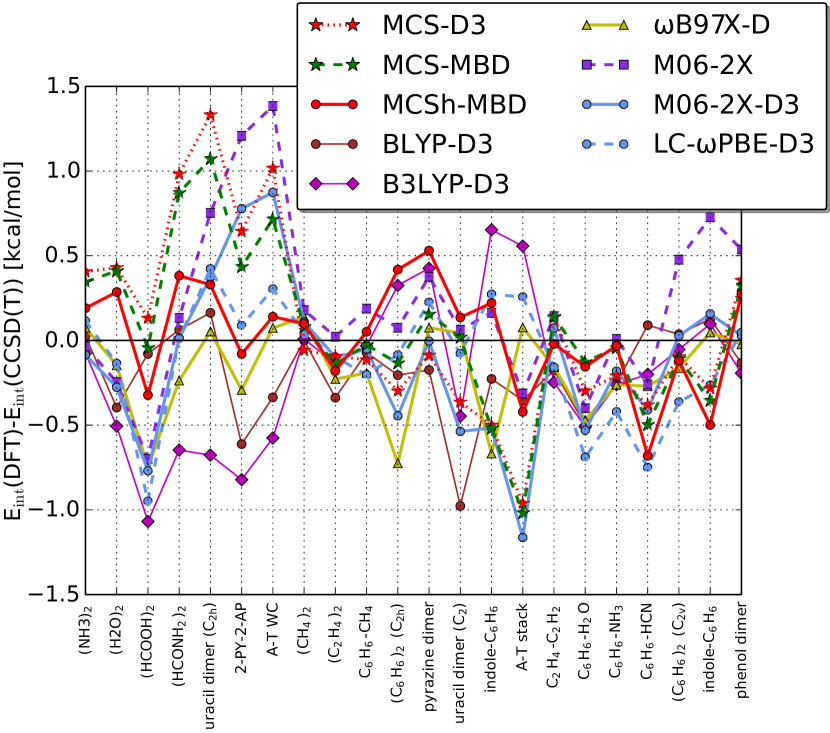
Figure 1: Detailed results for the S22 database. The deviations are with respect to the CCSD(T) results of Podeszwa, Patkowski, and Szalewicz (2010) The energies for the functionals other than MCS are taken from Goerigk and Grimme (2011). 2-PY-2-AP denotes 2-pyridone…2-aminopyridine.

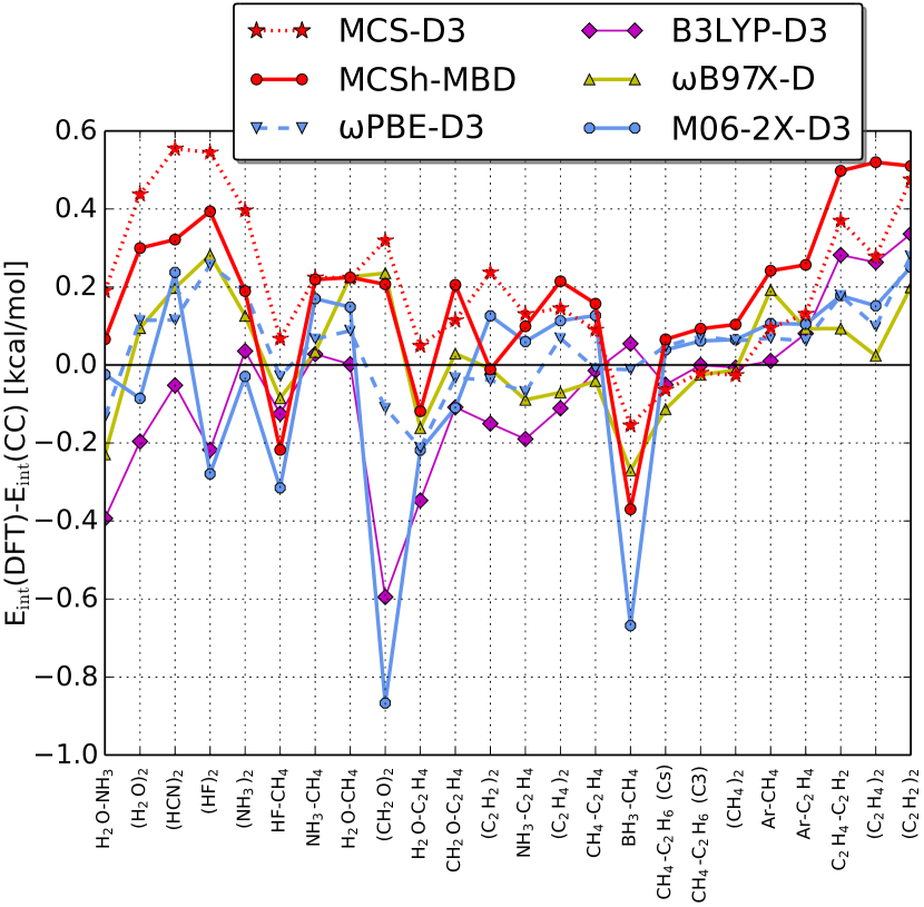
Figure 2: Detailed results for the A24 database. The deviations are with respect to the nonrelativistic interaction energies at the CCSD(T)/CBS level plus CCSDT(Q) corrections.Rezac and Hobza (2013) The energies for the functionals other than MCS are taken from Li, Muddana, and Gilson (2014)

Table 4: Statistical errors for the S22 and A24 databases.Jurecka et al. (2006); Rezac and Hobza (2013) The units are kcal/mol.

	MAPD	RMSD	MAD	MSD
S22
MCS-D3	7.05	0.54	0.42	0.08
MCS-MBD	6.05	0.47	0.34	0.07
MCSh-D3	5.44	0.44	0.34	0.15
MCSh-MBD	5.94	0.31	0.25	0.03
$\omega$PBE-D3	6.65	0.36	0.27	-0.11
M06-2X	7.38	0.53	0.38	0.20
M06-2X-D3	6.39	0.47	0.34	-0.12
B3LYP	86.4	4.91	3.76	3.76
B3LYP-D3	6.68	0.48	0.39	-0.20
BLYP-D3	5.41	0.33	0.24	-0.20
$\omega$B97X-D	7.37	0.32	0.23	-0.18
A24
MCS-D3	16.38	0.27	0.22	0.20
MCS-MBD	23.67	0.30	0.27	0.24
MCSh-D3	16.45	0.27	0.21	0.21
MCSh-MBD	22.82	0.27	0.23	0.17
$\omega$PBE-D3	8.06	0.12	0.10	0.05
M06-2X	20.51	0.29	0.23	0.04
M06-2X-D3	14.47	0.27	0.19	-0.03
B3LYP	99.6	1.10	1.00	1.00
B3LYP-D3	9.58	0.21	0.15	-0.06
$\omega$B97X-D	10.05	0.15	0.12	0.03

Table 5: Comparison of the D3 dispersion correction and SAPT dispersion plus exchange-dispersion for selected complexes from the S22 database. The SAPT dispersion energies are taken from Pernal et al. (2009) The units are kcal/mol.

dimer	SAPT	B3LYP-D3	MCS-D3	BLYP-D3
(CH4)_2	-1.06	-0.92	-0.79	-1.18
(C_2H_4)_2	-2.58	-2.12	-1.52	-2.90
uracil dimer stack	-11.08	-9.16	-6.87	-11.52
C6H6-H2O	-2.82	-2.32	-1.73	-2.89
C6H6-NH3	-2.86	-2.36	-1.76	-2.91

IV.2 Water clusters

Water clusters constitute a challenge for approximate DFT methods. Although water molecules are polar, their clusters are bound not only by electrostatics and induction, but also largely by the dispersion effects. More importantly, the clusters sample interactions not represented in the standard test databases: interactions with distant neighbors and multiple hydrogen bonds formed by a single water molecule.

Water clusters exemplify the advantage of our approach over the dispersion-corrected functionals based on massive error cancellation. Fig. 3 shows the system-size dependence of the errors of various methods. The MCS functionals show no systematic underbinding or overbinding. This is in contrast to the functionals based on the B88 exchange: B3LYP systematically underbinds, while both B3LYP-D3 and BLYP-D3 systematically overbind due to the overcorrection of the B88 exchange by the D3 term. This error cancellation had no adverse effects in the previous test cases.

Table 6 illustrates that all four MCS functionals yield exceptionally small relative and absolute errors for (H2O)_n with $n=2,\ldots,10$. While the choice of the dispersion correction does not influence the average errors, the choice of the exchange functional is more important. The hybrid MCS functionals perform significantly better than the pure counterparts. Of all the tested functionals, MCSh-MBD offers the best performance for the water clusters of Fig. 3.

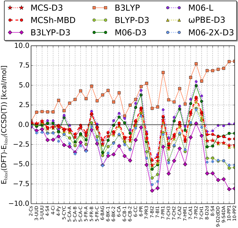
Figure 3: Differences between the CCSD(T)/CBS and DFT binding energies for (H2O)_n with $n=2,\ldots,10$. The coordinates, reference energies, and labels of the water clusters are taken from Temelso, Archer, and Shields (2011)

Table 6: Statistical errors of DFT methods for (H2O)_n with $n=2,\ldots,10$. The units are kcal/mol.

Functional	MAD	MAPD	MSD	RMSD
MCS-D3	1.53	3.17	-0.94	1.92
MCS-MBD	1.52	3.12	-1.02	1.91
MCSh-D3	1.25	2.92	0.87	1.69
MCSh-MBD	1.28	2.65	-0.59	1.64
M06-D3	1.71	3.58	-0.43	2.22
M06-2X-D3	2.75	5.79	-2.58	3.35
B3LYP	4.01	8.53	4.01	4.52
B3LYP-D3	3.66	7.39	-3.65	4.39
BLYP-D3	2.42	4.68	-2.18	3.04
$\omega$PBE-D3	1.55	3.06	-1.09	1.97
M06-L	1.40	3.13	0.29	1.98

Figs. 4 and 5 focus on the performance of approximate methods for water hexamers and 16-mers. All the MCS functionals yield small absolute errors, excellent ordering of the hexamers, and well reproduced (although not perfectly) tiny energy differences between the 16-mers. The effect of changing the dispersion correction is negligible when the exchange is pure ($\alpha=0$). However, there is an appreciable difference between MCSh-D3 and MCSh-MBD for the water 16-mers. While the binding energy for MCSh-MBD agrees almost perfectly with the reference values, MCSh-D3 underbinds by about $4\text{\,}\mathrm{k}\mathrm{c}\mathrm{a}\mathrm{l}\mathrm{/}\mathrm{m}\mathrm{o}\mathrm{l}$.

The excellent performance of the MCS functionals for the 16-mers is encouraging because these systems exhibit features that are expected in even larger clusters. First, among the systems considered in this study, only the 16-mers contain water molecules participating in four hydrogen bonds. Moreover, the energetics of the 16-mers include significant many-body effects, which are large compared to the energy differences between the isomers. Indeed, Wang, Deible, and Jordan (2013) have estimated that the 5-body and higher effects in the 4444-a 16-mer to contribute $-2.3\text{\,}\mathrm{k}\mathrm{c}\mathrm{a}\mathrm{l}\mathrm{/}\mathrm{m}\mathrm{o}\mathrm{l}$ to the binding energy at the MP2 level. This is a highly probable estimate since in our computations the MP2 method is shown to approach extremely close the CCSD(T)/CBS limits for all 16-mers (see Table 7).

Many-body effects in the 16-mers are dominated by induction terms, as shown by several studies on trimers of polar molecules.Szcześniak and Chałasiński (1992); Szcześniak, Kendall, and Chałasiński (1991); Chałasiński et al. (1991) This explains why the performance of MP2 is excellent for the 16-mers despite inability of MP2 to recover the third-order triple-dipole dispersion terms. The induction nature of many-body effects justifies the D3 atom-pairwise dispersion correction, which does not comprise any nonadditive three-body dispersion terms.Grimme et al. (2010) In fact, we have not observed any significant improvement attributable to the MBD dispersion correction which is capable of recovering many-body dispersion.

It should be emphasized that our reference binding energies of the 16-mers are uniformly shifted with respect to those used by Leverentz, Qi, and Truhlar (2013) This is because these authors employed the CCSD(T)/aug-cc-pVTZ energies of Yoo et al. (2010) as their final reference values, whereas in our study these energies have been refined in the extrapolation scheme defined in Eq. 28. The extrapolation has introduced an upward shift of about $6.5\text{\,}\mathrm{k}\mathrm{c}\mathrm{a}\mathrm{l}\mathrm{/}\mathrm{m}\mathrm{o}\mathrm{l}$ relative to CCSD(T)/aug-cc-pVTZ. A recent quantum Monte Carlo result of Wang, Deible, and Jordan (2013) for the 4444-a isomer ($-165.1(8)\text{\,}\mathrm{k}\mathrm{c}\mathrm{a}\mathrm{l}\mathrm{/}\mathrm{m}\mathrm{o}\mathrm{l}$) is in excellent agreement with our CCSD(T)/CBS extrapolation ($-164.51\text{\,}\mathrm{k}\mathrm{c}\mathrm{a}\mathrm{l}\mathrm{/}\mathrm{m}\mathrm{o}\mathrm{l}$).

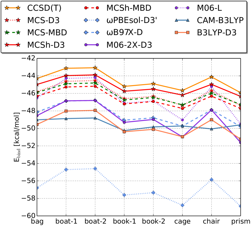
Figure 4: Binding energies of water hexamers. The coordinates and reference CCSD(T)/CBS energies are taken from Bates and Tschumper (2009). The energies for the functionals other than MCS are taken from Leverentz, Qi, and Truhlar (2013)

Table 7: Binding energies of water 16-mers. The CCSD(T) and RI-MP2 energies are extrapolated according to Eq. 28 and Eq. 29, respectively. The units are kcal/mol.

system	CCSD(T)	RI-MP2	MCS-D3	MCSh-MBD
4444-a	-164.51	-163.91	-166.54	-164.55
4444-b	-163.97	-163.46	-166.37	-164.24
antiboat	-164.11	-164.07	-166.48	-164.88
boat-a	-164.40	-164.45	-166.99	-165.36
boat-b	-164.28	-164.33	-166.79	-165.17

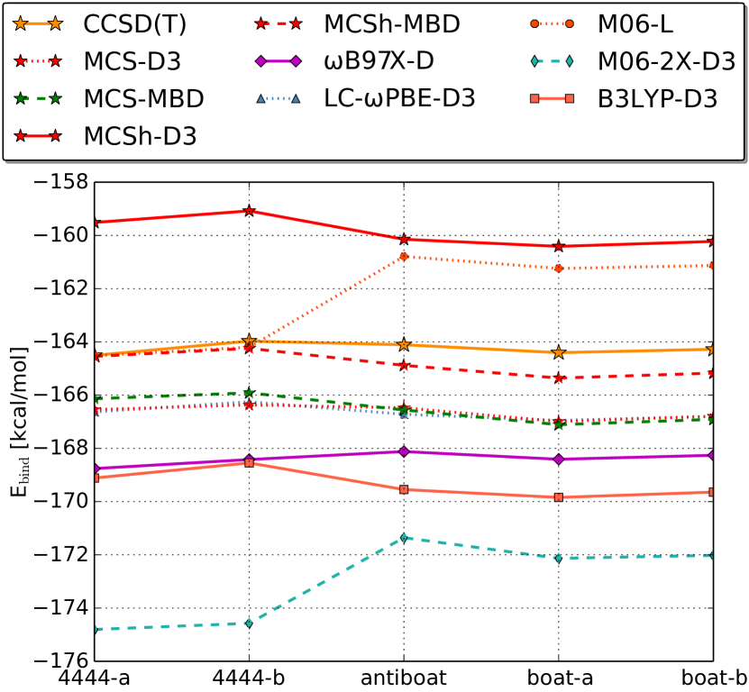
Figure 5: Binding energies of water 16-mers. The coordinates are taken from Yoo et al. (2010). The energies for the functionals other than MCS are taken from Leverentz, Qi, and Truhlar (2013).

IV.3 Ionic hydrogen bonds

Hydrogen-bonded systems composed of an ion interacting with a closed-shell molecule provide a simple model of interactions ubiquitous in biochemistry. From the point of view of dispersion corrections, charged dimers belong to the hardest cases: if a dispersion correction does not depend on the density, it will not reflect any alterations of dispersion due to the density change from a neutral to an ion, which is often dramatic. This is the case of the D3 model which has been parametrized within a set of neutral dimers, and its input consists of atomic coordinates only.Grimme, Hujo, and Kirchner (2012) However, because the total interaction is dominated by electrostatic and induction components, this weakness may not be especially relevant, as dispersion itself is relatively small and thus its accuracy not critical.

Figs. 6 and 7 show the performance of MCSh-MBD and compare this functional with the results of popular DFT methods. The differences between MCSh-MBD, B3LYP-D3, M06-2X-D3, and $\omega$B97X-D are small, and all of the curves are close to the reference ones. The $\omega$PBE-D3 functional is consistently worse than any of the MCS functionals (see Table 8) despite its good performance for water clusters.

Table 8 shows that switching from D3 to MBD changes little when applied with the pure MCS functionals. However, the choice the dispersion correction appears more important for the hybrid variants, and the MBD model works better in this case. This observation is consistent with our findings for the hydrogen-bonded dimers of the S22 database and for water clusters.

Table 8: Interaction energies of ionic hydrogen-bonded dimers at the equilibrium distances. The units are kcal/mol.

dimer	CCSD(T)	MCS-D3	MCS-MBD	MCSh-D3	MCSh-MBD	$\omega$PBE-D3
acetate…X
methanol	-19.75	-19.46	-19.57	-19.28	-19.74	-18.82
water	-21.06	-20.97	-21.15	-20.73	-21.22	-20.71
methylamine	-11.46	-10.96	-11.01	-10.85	-11.20	-10.45
imidazolium…X
formaldehyde	-16.41	-15.84	-15.86	-15.94	-16.14	-15.75
methylamine	-25.98	-26.58	-26.62	-26.69	-27.04	-26.86
water	-16.49	-16.25	-16.30	-16.30	-16.54	-15.89

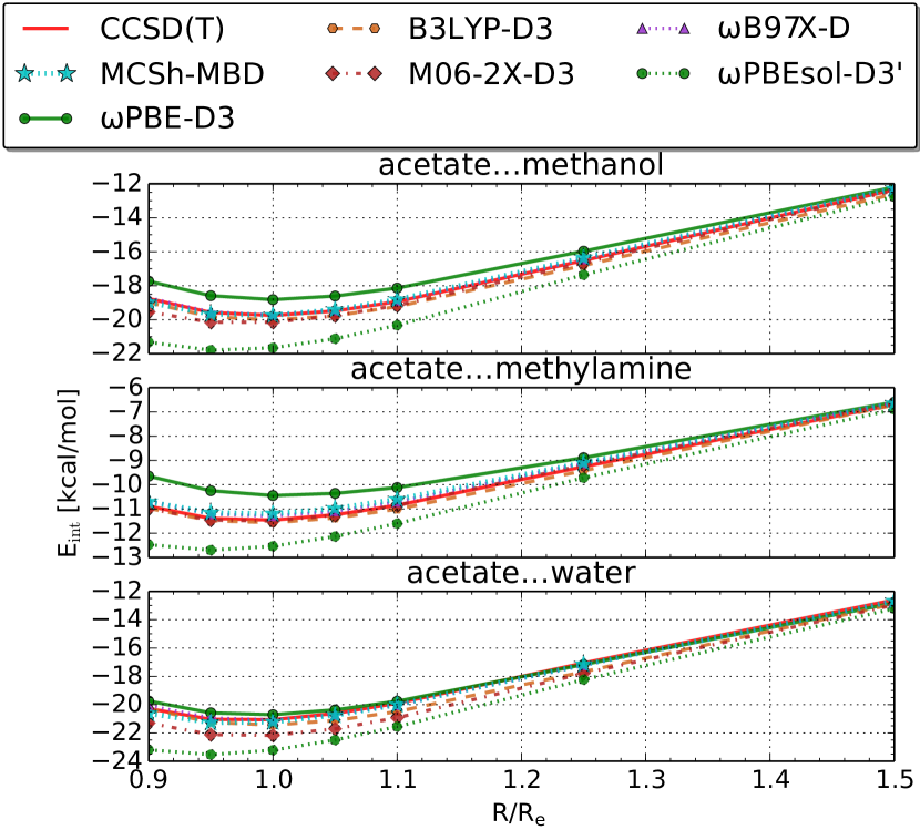
Figure 6: Interaction energy curves for hydrogen-bonded dimers including the acetate anion. The data for B3LYP-D3, M06-2X-D3, and B97X-D are taken from Ref. 47.

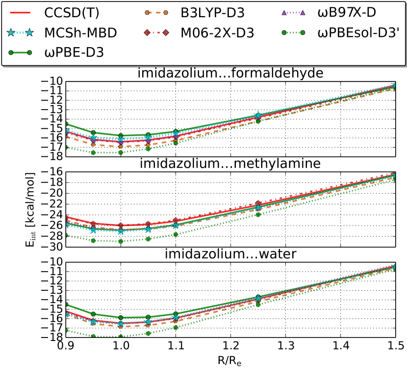
Figure 7: Interaction energy curves for hydrogen-bonded dimers including the imidazolium cation. The data for B3LYP-D3, M06-2X-D3, and B97X-D are taken from Ref. 47.

IV.4 Isodesmic reaction of n-alkanes

The systematic errors of DFT approximations in predicting alkane thermochemistry were discussed by Wodrich, Corminboeuf, and von Ragué Schleyer (2006), Song et al. (2010), and Grimme (2010). They observed that there is a substantial error in reaction energies of isodesmic ethane fragmentation reactions of alkanes, which accumulates as the chain length grows,

$$\ce{CH3(CH2)_{m}CH3+mCH4->(m+1)C2H6}.$$ (30)

The performance of approximate functionals for these reactions is connected to the quality of the description of noncovalent interactions. Johnson, Contreras-García, and Yang (2012) found that the error in the reactions of Eq. 30 has its origin in the region of space between 1,3 methylene groups where the reduced density gradient changes upon fragmentation of an alkane to ethane. This change is a signature of noncovalent bonds.Johnson et al. (2010)

Previous studies identified the features that a functional should possess to alleviate this problem: (i) range-separation of the exchange functional,Song et al. (2010) (ii) restoration of the exact gradient expansion of the exchangeCsonka et al. (2008) (as in PBEsol), (iii) a dispersion correction.Song et al. (2010); Grimme (2010) The MCS functionals as well as $\omega$PBEsol-D3’ (discussed in the next section) include all of the above features. As shown in Fig. 8, these methods are by far the best performers for reactions in question.

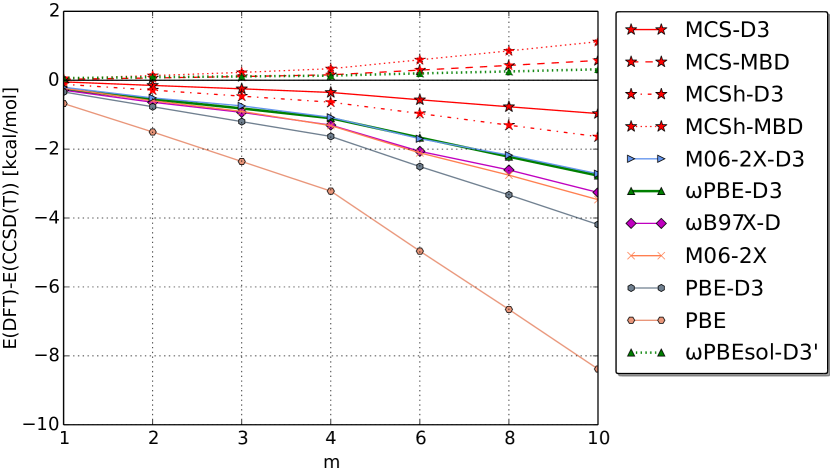
Figure 8: Errors in the energy of the isodesmic reaction. The reference energies and coordinates are taken from Grimme (2010).

IV.5 Merit of the MCS correlation

The question remains as to whether the correlation functional of our approach is indeed crucial to the quality of the above presented results. One might argue that this accuracy is primarily determined by the exchange and dispersion parts, and only weakly dependent on the semilocal correlation. To verify this hypothesis, we have composed a functional which differs from MCS-D3 only by the PBEsol correlation (denoted as $\omega$PBEsol-D3’), that is, both MCS-D3 and $\omega$PBEsol-D3’ share the same $\omega$PBEsol exchange with $\omega=0.3$ and the same D3 correction. Fig. 4 shows that keeping the PBEsol correlation leads to ca. $25\%$ overbinding in the case of water hexamers. A similar overbinding occurs for the 16-mers (e.g. $E_{\mathrm{bind}}=$-206.1\text{\,}\mathrm{k}\mathrm{c}\mathrm{a}\mathrm{l}\mathrm{/}\mathrm{m}\mathrm{o}\mathrm{l}$$ for the isomer 4444-a). Furthermore, $\omega$PBEsol-D3’ overestimates the interaction energies for every ionic hydrogen-bonded dimer presented in Figs. 6 and 7. Evidently, the role of the MCS correlation is essential in these examples, and its replacement by the standard PBEsol correlation leads to serious overestimation of interaction energies.

Nonetheless, it is of note that there exist cases where the choice of a semilocal correlation part matters less. For alkane fragmentation reactions, Fig. 8, $\omega$PBEsol-D3’ performs even better than the MCS functionals, which suggests the dominant role of the $\omega$PBEsol exchange in this case.

V Summary and conclusions

We have proposed a new DFT exchange-correlation functional that is specifically optimized for noncovalent interactions. It is composed of well-defined and physically meaningful components, with minimum of empiricism and reduced opportunity for error cancellation. It is built of the meta-GGA correlation functional developed by Modrzejewski et al. (2012) and the range-separated PBEsol exchange. The exchange and correlation contain a slight amount of empiricism in a form of parameters defining the scope of various approximations: a single parameter which governs damping of the semilocal correlation hole at large $r_{12}$, a range-separation parameter controlling the onset of the long-range HF exchange, and—in the case of the hybrid exchange—a fraction of the short-range HF exchange.

The novel piece of our functional, the correlation functional, is designed with the constraint satisfaction technique, but with the aid of its single empirical parameter it may be finely adjusted to any accurate variant of a dispersion correction without compromising any formal or physical constraints that it satisfies.

We have calibrated two long-range dispersion corrections to work with the remaining part of the functional: D3Grimme et al. (2010) and MBD.Ambrosetti et al. (2014) Taking into account the two possible variants of exchange and the two variants of dispersion, there is a set of four MCS functionals which are tested in this study.

The test set is composed of popular databases of small noncovalent dimers, but includes also the more demanding cases of water clusters, hydrogen-bonded interactions in ion-neutral pairs, and the thermochemistry of isodesmic reactions of n-alkanes. For the classic S22 database, the MCS functionals perform on a par or better than the leading functionals in the field of noncovalent interactions: B3LYP-D3, M06-2X-D3, and $\omega$B97X-D. More importantly, the MCS functionals perform markedly better than these functionals for large water clusters for which they successfully predict the binding energies from the newly refined CCSD(T)/CBS benchmarks. The good performance for hydrogen bonding extends to ionic hydrogen bonds. Finally, all four MCS functionals display excellent performance in predicting the energetics of isodesmic reactions of n-alkanes in direct consequence of the good description of the intramolecular interactions between methylene groups. We find that the PBEsol exchange combined with range separation and a dispersion correction essentially solves the known problems of DFT with isodesmic reactions of alkanes.

In view of the presented results, all four MCS functionals could be recommended for the description of noncovalent systems. The best performer in any case except few-atom dispersion-bound systems is MCSh-MBD.

VI Acknowledgments

This work was supported by the National Science Foundation (Grant No. CHE-1152474) and by the Polish Ministry of Science and Higher Education (Grant No. N204 248440). M.M. and G.C. gratefully acknowledge additional financial support from the Foundation for Polish Science. Special thanks to Aleksandra Tucholska for creating the TOC graphic for this paper.

Figure 9: For table of contents only

References

- Burns et al. (2011) L. A. Burns, A. Vazquez-Mayagoitia, B. G. Sumpter, and C. D. Sherrill, J. Chem. Phys. 134, 084107 (2011).
- Podeszwa and Szalewicz (2012) R. Podeszwa and K. Szalewicz, J. Chem. Phys. 136, 161102 (2012).
- Modrzejewski et al. (2012) M. Modrzejewski, M. Lesiuk, Ł. Rajchel, M. M. Szcz\textpolhookeśniak, and G. Chałasiński, J. Chem. Phys. 137, 204121 (2012).
- Perdew et al. (2008) J. P. Perdew, A. Ruzsinszky, G. I. Csonka, O. A. Vydrov, G. E. Scuseria, L. A. Constantin, X. Zhou, and K. Burke, Phys. Rev. Lett. 100, 136406 (2008).
- Csonka et al. (2008) G. I. Csonka, A. Ruzsinszky, J. P. Perdew, and S. Grimme, J. Chem. Theory Comput. 4, 888 (2008).
- Henderson, Janesko, and Scuseria (2008) T. M. Henderson, B. G. Janesko, and G. E. Scuseria, J. Chem. Phys. 128, 194105 (2008).
- Grimme et al. (2010) S. Grimme, J. Antony, S. Ehrlich, and H. Krieg, J. Chem. Phys. 132, 154104 (2010).
- Ambrosetti et al. (2014) A. Ambrosetti, A. M. Reilly, R. A. DiStasio Jr, and A. Tkatchenko, J. Chem. Phys. 140, 18A508 (2014).
- Lee et al. (2010) K. Lee, É. Murray, L. Kong, B. Lundqvist, and D. Langreth, Phys. Rev. B 82, 081101 (2010).
- Vydrov and Van Voorhis (2010) O. Vydrov and T. Van Voorhis, J. Chem. Phys. 133, 244103 (2010).
- Sato and Nakai (2010) T. Sato and H. Nakai, J. Chem. Phys. 133, 194101 (2010).
- Becke and Johnson (2005) A. Becke and E. Johnson, J. Chem. Phys. 122, 154104 (2005).
- Lacks and Gordon (1993) D. J. Lacks and R. G. Gordon, Phys. Rev. A 47, 4681 (1993).
- Murray, Lee, and Langreth (2009) E. D. Murray, K. Lee, and D. C. Langreth, J. Chem. Theory Comput. 5, 2754 (2009).
- Johnson et al. (2010) E. R. Johnson, S. Keinan, P. Mori-Sanchez, J. Contreras-Garcia, A. J. Cohen, and W. Yang, J. Am. Chem. Soc. 132, 6498 (2010).
- Kannemann and Becke (2009) F. O. Kannemann and A. D. Becke, J. Chem. Theory Comput. 5, 719 (2009).
- Kamiya, Tsuneda, and Hirao (2002) M. Kamiya, T. Tsuneda, and K. Hirao, J. Chem. Phys. 117, 6010 (2002).
- Johnson, Contreras-García, and Yang (2012) E. R. Johnson, J. Contreras-García, and W. Yang, J. Chem. Theory Comput. 8, 2676 (2012).
- Misquitta et al. (2005) A. Misquitta, R. Podeszwa, B. Jeziorski, and K. Szalewicz, J. Chem. Phys. 123, 214103 (2005).
- Chai and Head-Gordon (2008) J.-D. Chai and M. Head-Gordon, Phys. Chem. Chem. Phys. 10, 6615 (2008).
- Lin et al. (2013) Y.-S. Lin, G.-D. Li, S.-P. Mao, and J.-D. Chai, J. Chem. Theory Comput. 9, 263 (2013).
- Mardirossian and Head-Gordon (2014) N. Mardirossian and M. Head-Gordon, J. Chem. Phys. 140, 18A527 (2014).
- Pernal et al. (2009) K. Pernal, R. Podeszwa, K. Patkowski, and K. Szalewicz, Phys. Rev. Lett. 103, 263201 (2009).
- Gori-Giorgi and Perdew (2001) P. Gori-Giorgi and J. Perdew, Phys. Rev. B 64, 155102 (2001).
- Rassolov, Pople, and Ratner (2000) V. Rassolov, J. Pople, and M. Ratner, Phys. Rev. B 62, 2232 (2000).
- Burke, Perdew, and Ernzerhof (1998) K. Burke, J. Perdew, and M. Ernzerhof, J. Chem. Phys. 109, 3760 (1998).
- Tkatchenko et al. (2012) A. Tkatchenko, R. A. DiStasio Jr, R. Car, and M. Scheffler, Phys. Rev. Lett. 108, 236402 (2012).
- Ruzsinszky et al. (2012) A. Ruzsinszky, J. P. Perdew, J. Tao, G. I. Csonka, and J. Pitarke, Phys. Rev. Lett. 109, 233203 (2012).
- Gobre and Tkatchenko (2013) V. V. Gobre and A. Tkatchenko, Nat. Commun. 4, 2341 (2013).
- Rohrdanz, Martins, and Herbert (2009) M. A. Rohrdanz, K. M. Martins, and J. M. Herbert, J. Chem. Phys. 130, 054112 (2009).
- Modrzejewski et al. (2013) M. Modrzejewski, Ł. Rajchel, G. Chałasiński, and M. M. Szcz\textpolhookeśniak, J. Phys. Chem. A 117, 11580 (2013).
- Koppen et al. (2014) J. V. Koppen, M. Hapka, M. Modrzejewski, M. M. Szczęśniak, and G. Chałasiński, J. Chem. Phys. 140, 244313 (2014).
- Perdew, Burke, and Ernzerhof (1996) J. Perdew, K. Burke, and M. Ernzerhof, Phys. Rev. Lett. 77, 3865 (1996).
- Stephens et al. (1994) P. J. Stephens, F. J. Devlin, C. F. Chabalowski, and M. J. Frisch, J. Phys. Chem. 98, 11623 (1994).
- Gill et al. (1992) P. M. Gill, B. G. Johnson, J. A. Pople, and M. J. Frisch, Chem. Phys. Lett. 197, 499 (1992).
- Zhao and Truhlar (2008) Y. Zhao and D. Truhlar, Theor. Chem. Acc. 120, 215 (2008).
- Vydrov et al. (2006) O. A. Vydrov, J. Heyd, A. V. Krukau, and G. E. Scuseria, J. Chem. Phys. 125, 074106 (2006).
- Weigend and Ahlrichs (2005) F. Weigend and R. Ahlrichs, Phys. Chem. Chem. Phys. 7, 3297 (2005).
- Schuchardt et al. (2007) K. L. Schuchardt, B. T. Didier, T. Elsethagen, L. Sun, V. Gurumoorthi, J. Chase, J. Li, and T. L. Windus, J. Chem. Inf. Model. 47, 1045 (2007).
- Zhao and Truhlar (2005a) Y. Zhao and D. Truhlar, J. Phys. Chem. A 109, 5656 (2005a).
- Zhao and Truhlar (2005b) Y. Zhao and D. Truhlar, J. Chem. Theory Comput. 1, 415 (2005b).
- Jurecka et al. (2006) P. Jurecka, J. Sponer, J. Cerny, and P. Hobza, Phys. Chem. Chem. Phys. 8, 1985 (2006).
- Rezac, Riley, and Hobza (2011) J. Rezac, K. E. Riley, and P. Hobza, J. Chem. Theory Comput. 7, 2427 (2011).
- Halkier et al. (1999) A. Halkier, W. Klopper, T. Helgaker, P. Jorgensen, and P. R. Taylor, J. Chem. Phys. 111, 9157 (1999).
- Valiev et al. (2010) M. Valiev, E. J. Bylaska, N. Govind, K. Kowalski, T. P. Straatsma, H. J. Van Dam, D. Wang, J. Nieplocha, E. Apra, T. L. Windus, and W. de Jong, Comput. Phys. Commun. 181, 1477 (2010).
- Yoo et al. (2010) S. Yoo, E. Apra, X. C. Zeng, and S. S. Xantheas, J. Phys. Chem. Lett. 1, 3122 (2010).
- Li, Muddana, and Gilson (2014) A. Li, H. S. Muddana, and M. K. Gilson, J. Chem. Theory Comput. 10, 1563 (2014).
- Rezac and Hobza (2013) J. Rezac and P. Hobza, J. Chem. Theory Comput. 9, 2151 (2013).
- Becke (1988) A. D. Becke, Phys. Rev. A 38, 3098 (1988).
- Podeszwa, Patkowski, and Szalewicz (2010) R. Podeszwa, K. Patkowski, and K. Szalewicz, Phys. Chem. Chem. Phys. 12, 5974 (2010).
- Goerigk and Grimme (2011) L. Goerigk and S. Grimme, Phys. Chem. Chem. Phys. 13, 6670 (2011).
- Temelso, Archer, and Shields (2011) B. Temelso, K. A. Archer, and G. C. Shields, J. Phys. Chem. A 115, 12034 (2011).
- Wang, Deible, and Jordan (2013) F.-F. Wang, M. J. Deible, and K. D. Jordan, J. Phys. Chem. A 117, 7606 (2013).
- Szcz\textpolhookeśniak and Chałasiński (1992) M. M. Szcz\textpolhookeśniak and G. Chałasiński, J. Mol. Struct. THEOCHEM 261, 37 (1992).
- Szcz\textpolhookeśniak, Kendall, and Chałasiński (1991) M. M. Szcz\textpolhookeśniak, R. A. Kendall, and G. Chałasiński, J. Chem. Phys. 95, 5169 (1991).
- Chałasiński et al. (1991) G. Chałasiński, M. M. Szcz\textpolhookeśniak, P. Cieplak, and S. Scheiner, J. Chem. Phys. 94, 2873 (1991).
- Leverentz, Qi, and Truhlar (2013) H. R. Leverentz, H. W. Qi, and D. G. Truhlar, J. Chem. Theory Comput. 9, 995 (2013).
- Bates and Tschumper (2009) D. M. Bates and G. S. Tschumper, J. Phys. Chem. A 113, 3555 (2009).
- Grimme, Hujo, and Kirchner (2012) S. Grimme, W. Hujo, and B. Kirchner, Phys. Chem. Chem. Phys. 14, 4875 (2012).
- Wodrich, Corminboeuf, and von Ragué Schleyer (2006) M. D. Wodrich, C. Corminboeuf, and P. von Ragué Schleyer, Org. Lett. 8, 3631 (2006).
- Song et al. (2010) J.-W. Song, T. Tsuneda, T. Sato, and K. Hirao, Org. Lett. 12, 1440 (2010).
- Grimme (2010) S. Grimme, Org. Lett. 12, 4670 (2010).