Measuring CP violation in Two-Higgs-Doublet models
in light of the LHC Higgs data

Abstract

In Two-Higgs-Doublet models, the conditions for CP violation can be expressed in terms of invariants under U(2) rotations among the two SU(2) Higgs doublet fields. In order to design a strategy for measuring the invariants we express them in terms of observables, i.e., masses and couplings of scalar bosons. We find amplitudes directly sensitive to the invariants. Observation of the Standard-Model-like Higgs boson at the LHC severely constrains the models. In particular, in the model with ${\mathbbm{Z}}_{2}$ symmetry imposed on dimension-4 terms (in order to eliminate tree-level flavour-changing neutral currents), CP violation is strongly suppressed. On the other hand, the most general Two-Higgs-Doublet model (without ${\mathbbm{Z}}_{2}$ symmetry) is compatible with the LHC data, and would still allow for CP violation to be present in the model. Consequently, also flavour-changing neutral currents would in general be expected. We briefly sketch a strategy for measuring the remaining CP violation.

1 Introduction

As is well known, the Two-Higgs-Doublet model (2HDM) allows for extra sources of CP violation that originate in the scalar potential. This possibility opens interesting perspectives for cosmology Riotto:1999yt . Nevertheless, this option receives little attention in much of the literature Branco:2011iw . The 2HDM can be formulated in any basis chosen for the Higgs doublets, e.g. any U(2) rotation acting upon the doublets $(\Phi_{1},\Phi_{2})$ would lead to an equivalent basis. Thus, physical implications, such as cross sections, decay widths etc., can only depend on quantities that are basis independent. In this paper we discuss CP violation originating from the scalar sector of the 2HDM. In order to present results in a basis independent way, we are going to study weak basis invariants sensitive to CP violation.

Necessary conditions for having CP violation in this model were first formulated in terms of invariants 20 years ago by Lavoura, Silva and Botella Lavoura:1994fv ; Botella:1994cs . More recently, this issue was addressed by Branco, Rebelo and Silva-Marcos Branco:2005em , by Gunion and Haber Gunion:2005ja and by Haber and O’Neil Haber:2006ue . Independent approaches have been presented both in terms of algebraic invariants Davidson:2005cw and geometric quantities Ivanov:2005hg ; Nishi:2006tg ; Ivanov:2006yq ; Maniatis:2007vn . Detailed discussions of CP-violating invariants are also contained in Branco:1999fs . These invariants are analogous to the Jarlskog invariant $J$ Jarlskog:1985ht describing CP violation induced by the Yukawa couplings in the Standard Model (SM).

There exist several versions of the 2HDM which differ by the Yukawa interactions, e.g. type I or type II 2HDM. Our intention in this paper is to present results which are type-independent, thus insensitive to the Yukawa structure, and hence applicable in any 2HDM. Therefore we are going to restrict ourselves to the bosonic sector of the model. The Yukawa sector will in general supply additional sources of CP violation.

The paper is organized as follows. In section 2 we review the model, and establish our notation. In section 3 we discuss CP violation, and present the criteria for CP violation in terms of physical couplings and masses. In section 4 we relate these invariants to physical amplitudes involving scalars and vector bosons. Then, in section 5 we discuss the limit in which the 125 GeV Higgs particle observed at the LHC Aad:2012tfa ; Chatrchyan:2012ufa is the lightest neutral Higgs boson of the model, and couples to vector bosons like the SM Higgs boson. We show that the most general 2HDM still allows for CP violation involving the heavier companions, and also that tree-level flavour violation in couplings of neutral scalars could be present. In section 6 we present some numerical illustrations, in section 7 we outline a strategy for systematically excluding or discovering CP violation in the model, and in section 8 we summarize our main points. Technical details are relegated to two appendices.

2 The model

The scalar potential of the 2HDM shall be parametrized in the standard fashion:

$$V(\Phi_{1},\Phi_{2}) =-\frac{1}{2}\left\{m_{11}^{2}\Phi_{1}^{\dagger}\Phi_{1}+m_{22}^{2}\Phi_{2}^{\dagger}\Phi_{2}+\left[m_{12}^{2}\Phi_{1}^{\dagger}\Phi_{2}+\hbox{H.c.}\right]\right\}$$

$$+\frac{\lambda_{1}}{2}(\Phi_{1}^{\dagger}\Phi_{1})^{2}+\frac{\lambda_{2}}{2}(\Phi_{2}^{\dagger}\Phi_{2})^{2}+\lambda_{3}(\Phi_{1}^{\dagger}\Phi_{1})(\Phi_{2}^{\dagger}\Phi_{2})+\lambda_{4}(\Phi_{1}^{\dagger}\Phi_{2})(\Phi_{2}^{\dagger}\Phi_{1})$$

$$+\frac{1}{2}\left[\lambda_{5}(\Phi_{1}^{\dagger}\Phi_{2})^{2}+\hbox{H.c.}\right]+\left\{\left[\lambda_{6}(\Phi_{1}^{\dagger}\Phi_{1})+\lambda_{7}(\Phi_{2}^{\dagger}\Phi_{2})\right](\Phi_{1}^{\dagger}\Phi_{2})+{\rm\hbox{H.c.}}\right\}$$ (2.1)

$$\equiv Y_{a\bar{b}}\Phi_{\bar{a}}^{\dagger}\Phi_{b}+\frac{1}{2}Z_{a\bar{b}c\bar{d}}(\Phi_{\bar{a}}^{\dagger}\Phi_{b})(\Phi_{\bar{c}}^{\dagger}\Phi_{d}).$$ (2.2)

In the second form, Eq. (2.2), a summation over barred with un-barred indices is implied, e.g., $a=\bar{a}=1,2$. Thus,

$$Y_{11}=-\frac{m_{11}^{2}}{2},\quad Y_{12}=-\frac{m_{12}^{2}}{2},\quad Y_{21}=-\frac{(m_{12}^{2})^{*}}{2},\quad Y_{22}=-\frac{m_{22}^{2}}{2}$$ (2.3)

and

$$Z_{1111}=\lambda_{1},\quad Z_{2222}=\lambda_{2},\quad Z_{1122}=Z_{2211}=\lambda_{3},$$

$$Z_{1221}=Z_{2112}=\lambda_{4},\quad Z_{1212}=\lambda_{5},\quad Z_{2121}=(\lambda_{5})^{*},$$

$$Z_{1112}=Z_{1211}=\lambda_{6},\quad Z_{1121}=Z_{2111}=(\lambda_{6})^{*},$$

$$Z_{1222}=Z_{2212}=\lambda_{7},\quad Z_{2122}=Z_{2221}=(\lambda_{7})^{*}.$$ (2.4)

All other $Z_{a\bar{b}c\bar{d}}$ vanish.

Usually a ${\mathbbm{Z}}_{2}$ symmetry is imposed on the dimension-4 terms in order to eliminate potentially large flavour-changing neutral currents in the Yukawa couplings. We will in the present work not restrict ourselves by imposing this symmetry, and therefore we are going to consider the most general scalar potential, keeping also terms that are not allowed by ${\mathbbm{Z}}_{2}$ symmetry.

In an arbitrary basis, the vacuum may be complex, and the Higgs doublets can be parameterized as

$$\Phi_{j}=e^{i\xi_{j}}\left(\begin{array}[]{c}\varphi_{j}^{+}\\ (v_{j}+\eta_{j}+i\chi_{j})/\sqrt{2}\end{array}\right),\quad j=1,2.$$ (2.5)

Here $v_{j}$ are real numbers, so that $v_{1}^{2}+v_{2}^{2}=v^{2}$. The fields $\eta_{j}$ and $\chi_{j}$ are real. The phase difference between the two vevs is given by

$$\xi\equiv\xi_{2}-\xi_{1}.$$ (2.6)

The vevs may also be written as

$$\left<\Phi_{j}\right>=\frac{1}{\sqrt{2}}\left(\begin{array}[]{c}0\\ v\hat{v}_{j}\end{array}\right).$$ (2.7)

where

$$\hat{v}_{1}=\frac{v_{1}}{v}e^{i\xi_{1}},\quad\hat{v}_{2}=\frac{v_{2}}{v}e^{i\xi_{2}},$$ (2.8)

which will be useful later. Next, let’s define orthogonal states

$$\left(\begin{array}[]{c}G_{0}\\ \eta_{3}\end{array}\right)=\left(\begin{array}[]{cc}v_{1}/v&v_{2}/v\\ -v_{2}/v&v_{1}/v\end{array}\right)\left(\begin{array}[]{c}\chi_{1}\\ \chi_{2}\end{array}\right)$$ (2.9)

and

$$\left(\begin{array}[]{c}G^{\pm}\\ H^{\pm}\end{array}\right)=\left(\begin{array}[]{cc}v_{1}/v&v_{2}/v\\ -v_{2}/v&v_{1}/v\end{array}\right)\left(\begin{array}[]{c}\varphi_{1}^{\pm}\\ \varphi_{2}^{\pm}\end{array}\right).$$ (2.10)

Then $G_{0}$ and $G^{\pm}$ become the massless Goldstone fields, and $H^{\pm}$ are the charged scalars.

The model also contains three neutral scalars, which are linear compositions of the $\eta_{i}$,

$$\begin{pmatrix}H_{1}\\ H_{2}\\ H_{3}\end{pmatrix}=R\begin{pmatrix}\eta_{1}\\ \eta_{2}\\ \eta_{3}\end{pmatrix},$$ (2.11)

with the $3\times 3$ orthogonal rotation matrix $R$ satisfying

$$R{\cal M}^{2}R^{\rm T}={\cal M}^{2}_{\rm diag}={\rm diag}(M_{1}^{2},M_{2}^{2},M_{3}^{2}),$$ (2.12)

and with $M_{1}\leq M_{2}\leq M_{3}$. A convenient parametrization of the rotation matrix $R$ is Accomando:2006ga ; El_Kaffas:2006nt

$$R=\begin{pmatrix}R_{11}&R_{12}&R_{13}\\ R_{21}&R_{22}&R_{23}\\ R_{31}&R_{32}&R_{33}\end{pmatrix}=\begin{pmatrix}c_{1}\,c_{2}&s_{1}\,c_{2}&s_{2}\\ -(c_{1}\,s_{2}\,s_{3}+s_{1}\,c_{3})&c_{1}\,c_{3}-s_{1}\,s_{2}\,s_{3}&c_{2}\,s_{3}\\ -c_{1}\,s_{2}\,c_{3}+s_{1}\,s_{3}&-(c_{1}\,s_{3}+s_{1}\,s_{2}\,c_{3})&c_{2}\,c_{3}\end{pmatrix}.$$ (2.13)

Since $R$ is orthogonal, only three of the elements $R_{ij}$ are independent. The rest can be expressed by these through the use of orthogonality relations. From the potential one can now derive expressions for the masses of the scalars as well as Feynman rules for scalar interactions. For a general basis that we consider here, these expressions are quite involved and lengthy so we have chosen to collect them in Appendix A.

3 CP violation

The addition of the second doublet triggers qualitatively new phenomena originating from interactions of scalar particles. The crucial one is the attractive possibility of CP violation in the scalar potential Lee:1973iz . This extra source of CP violation might be very essential for explaining the baryon asymmetry. In this section we are going to discuss parametrization of CP violation in terms of weak-basis invariants.

3.1 Conditions for CP violation

As pointed out by Gunion and Haber, the conditions for having CP violation in the model can be expressed in terms of three U(2) invariants constructed from coefficients of the quadratic ($Y$) and dimension-4 ($Z$) terms of the potential, together with the vacuum expectation values.

It was found Gunion:2005ja that in order to break CP at least one of following three invariants had to be non-zero:

$$\mbox{Im\thinspace}J_{1} =-\frac{2}{v^{2}}\mbox{Im\thinspace}\bigl{[}\hat{v}_{\bar{a}}^{*}Y_{a\bar{b}}Z_{b\bar{d}}^{(1)}\hat{v}_{d}\bigr{]},$$ (3.1a)

$$\mbox{Im\thinspace}J_{2} =\frac{4}{v^{4}}\mbox{Im\thinspace}\bigl{[}\hat{v}_{\bar{b}}^{*}\hat{v}_{\bar{c}}^{*}Y_{b\bar{e}}Y_{c\bar{f}}Z_{e\bar{a}f\bar{d}}\hat{v}_{a}\hat{v}_{d}\bigr{]},$$ (3.1b)

$$\mbox{Im\thinspace}J_{3} =\mbox{Im\thinspace}\bigl{[}\hat{v}_{\bar{b}}^{*}\hat{v}_{\bar{c}}^{*}Z_{b\bar{e}}^{(1)}Z_{c\bar{f}}^{(1)}Z_{e\bar{a}f\bar{d}}\hat{v}_{a}\hat{v}_{d}\bigr{]},$$ (3.1c)

where $Z_{a\bar{d}}^{(1)}\equiv\delta_{b\bar{c}}Z_{a\bar{b}c\bar{d}}$. Having invariants expressed by the parameters of the potential and the vevs, one is faced with the challenge of measuring all these parameters in order to determine the CP properties of the model Grzadkowski:2013rza . For this purpose it would be much more convenient to formulate the conditions for CP violation in terms of physically measurable quantities like masses and couplings.

3.2 Expressing $\mbox{Im\thinspace}J_{i}$ in terms of masses and couplings

Our aim is to express $\mbox{Im\thinspace}J_{i},$ $i=1,2,3$ in terms of physical quantities. We shall start by first writing out these expressions explicitly in terms of the parameters of the potential and the vevs. Then we will re-express the original parameters of the potential in terms of another set of parameters :

$${\cal P}_{67}\equiv\{M_{H^{\pm}}^{2},\mu^{2},M_{1}^{2},M_{2}^{2},M_{3}^{2},{\rm Im}\lambda_{5},{\rm Re}\lambda_{6},{\rm Re}\lambda_{7},v_{1},v_{2},\xi,\alpha_{1},\alpha_{2},\alpha_{3}\}.$$ (3.2)

See Appendix A for details.

The resulting expressions are large, but can be handled efficiently by computer algebra. We used Mathematica mathematica for this purpose. Using (A.1)–(A.3) along with (A.18)–(A.2), we are able to express $\mbox{Im\thinspace}J_{i}$ in terms of the parameters ${\cal P}_{67}$ listed in (3.2). It is also worth noticing that each of the $\mbox{Im\thinspace}J_{i}$ is a homogeneous polynomial in a subset of ${\cal P}_{67}$ defined as

$${\cal P}_{0}=\{M_{H^{\pm}}^{2},\mu^{2},M_{1}^{2},M_{2}^{2},M_{3}^{2},{\rm Im}\lambda_{5},{\rm Re}\lambda_{6},{\rm Re}\lambda_{7}\},$$ (3.3)

for details see (A.18)–(A.2). In particular, $\mbox{Im\thinspace}J_{1}$ is of order 2, whereas $\mbox{Im\thinspace}J_{2}$ and $\mbox{Im\thinspace}J_{3}$ are of order 3. This means that by expanding these expressions in the parameters of ${\cal P}_{0}$, we get 36 terms in the expansion of $\mbox{Im\thinspace}J_{1}$ and 120 terms in the expansions of $\mbox{Im\thinspace}J_{2}$ and $\mbox{Im\thinspace}J_{3}$.

We denote the couplings $(H_{i}VV)$, $(H_{i}H^{+}H^{-})$ and $(H^{+}H^{-}H^{+}H^{-})$, by $e_{i}$, $q_{i}$ and $q$, respectively, details are contained in Appendix B.

Let us start by investigating $\mbox{Im\thinspace}J_{2}$, since this turns out to be the simplest of the three invariants. By writing out all the 120 terms of this invariant, using the orthogonality of the rotation matrix, we find that the terms containing $M_{H^{\pm}}^{2},\mu^{2},{\rm Im}\lambda_{5},{\rm Re}\lambda_{6},{\rm Re}\lambda_{7}$ all vanish. The resulting expression becomes

$$\mbox{Im\thinspace}J_{2} = \frac{2e_{1}e_{2}e_{3}}{v^{9}}(M_{1}^{2}-M_{2}^{2})(M_{2}^{2}-M_{3}^{2})(M_{3}^{2}-M_{1}^{2})$$ (3.4)

$$= \frac{2}{v^{9}}\sum_{i,j,k}\epsilon_{ijk}e_{i}e_{j}e_{k}M_{i}^{4}M_{k}^{2}=\frac{2e_{1}e_{2}e_{3}}{v^{9}}\sum_{i,j,k}\epsilon_{ijk}M_{i}^{4}M_{k}^{2}.$$

We note that this expression is completely antisymmetric under the interchange of two of the indices $i,j,k$, labeling the three neutral Higgs fields. The above formula found in the general basis confirms the result obtained in the “Higgs basis” ($v_{1}=v$ and $v_{2}=0$) in Lavoura:1994fv .

Next, we turn to $\mbox{Im\thinspace}J_{1}$. By writing out all the 36 terms of this invariant, using the orthogonality of the rotation matrix, we find that terms not containing neutral Higgs masses vanish. Also, the terms containing $M_{i}^{4}$ vanish in this expansion. Inspired by the results for $\mbox{Im\thinspace}J_{2}$, we conjectured that also the expression for $\mbox{Im\thinspace}J_{1}$ should be completely antisymmetric under the exchange of two of the indices $i,j,k$. A careful study of the coefficients of $\mbox{Im\thinspace}J_{1}$ in the expansion of parameters of ${\cal P}_{0}$ suggests we look for an expression proportional to $\sum_{i,j,k}\epsilon_{ijk}e_{i}^{a}e_{j}^{b}e_{k}^{c}M_{i}^{2}q_{j}$ which is of order 2 in the parameters of ${\cal P}_{0}$. Under this conjecture, we tried out different small values of $a,b,c$, seeing if we could reproduce the expression for $\mbox{Im\thinspace}J_{1}$. After a small game of trial and error we hit the jackpot by putting $a=c=1$ and $b=0$, establishing the relation

$$\mbox{Im\thinspace}J_{1} = \frac{1}{v^{5}}\sum_{i,j,k}\epsilon_{ijk}M_{i}^{2}e_{i}e_{k}q_{j}$$ (3.5)

$$= \frac{1}{v^{5}}[M_{1}^{2}e_{1}(e_{3}q_{2}-e_{2}q_{3})+M_{2}^{2}e_{2}(e_{1}q_{3}-e_{3}q_{1})+M_{3}^{2}e_{3}(e_{2}q_{1}-e_{1}q_{2})].$$

$\mbox{Im\thinspace}J_{3}$ turns out to be more complex. In fact it contains some terms with $\mbox{Im\thinspace}J_{1}$ and $\mbox{Im\thinspace}J_{2}$ plus “independent” terms. We have established the following identity

$$\mbox{Im\thinspace}J_{3}=K\,\mbox{Im\thinspace}J_{1}+\mbox{Im\thinspace}J_{2}+\frac{2}{v^{7}}\sum_{i,j,k}\epsilon_{ijk}(v^{2}q_{i}+2e_{i}M_{i}^{2})M_{i}^{2}e_{j}q_{k}$$ (3.6)

with

$$K =\frac{2}{v^{4}}\left[(e_{1}^{2}M_{1}^{2}+e_{2}^{2}M_{2}^{2}+e_{3}^{2}M_{3}^{2})+v^{2}(e_{1}q_{1}+e_{2}q_{2}+e_{3}q_{3})+2v^{2}M_{H^{\pm}}^{2}\right]$$

$$=\frac{2}{v^{4}}\left[(e_{1}^{2}M_{1}^{2}+e_{2}^{2}M_{2}^{2}+e_{3}^{2}M_{3}^{2})+2v^{4}\sigma-4v^{4}q+2v^{2}M_{H^{\pm}}^{2}\right],$$ (3.7)

where $\sigma$ and $q$ are defined in equations (B.11) and (B.7).

By putting all the $\mbox{Im\thinspace}J_{i}=0$ and solving the resulting three equations, we arrive at six distinct cases under which we have CP conservation:

Case 1: $M_{1}=M_{2}=M_{3}$. Full mass degeneracy.
Case 2: $M_{1}=M_{2}$ and $e_{1}q_{2}=e_{2}q_{1}$.
Case 3: $M_{2}=M_{3}$ and $e_{2}q_{3}=e_{3}q_{2}$.
Case 4: $e_{1}=0$ and $q_{1}=0$.
Case 5: $e_{2}=0$ and $q_{2}=0$.
Case 6: $e_{3}=0$ and $q_{3}=0$.

The obvious solution $e_{1}=e_{2}=e_{3}=0$ is not included since $e_{1}^{2}+e_{2}^{2}+e_{3}^{2}=v^{2}\neq 0$, and this solution would be unphysical. If one (or more) of the 6 above cases occur, it means that the 2HDM is CP conserving. If none of the above cases occurs, it means that the 2HDM violates CP. It is worth noticing that the nature of CP violation is not revealed at this point, i.e., CP could be broken explicitly or spontaneously Grzadkowski:2013rza .

3.3 Re-expressing the conditions for CP violation

While $\mbox{Im\thinspace}J_{1}$ and $\mbox{Im\thinspace}J_{2}$ are somewhat “atomic” in form when written as an antisymmetric sum, $\mbox{Im\thinspace}J_{3}$ is not. Let us therefore focus on the “independent” terms in the expression for $\mbox{Im\thinspace}J_{3}$, and split them like

$$\frac{2}{v^{7}}\sum_{i,j,k}\epsilon_{ijk}(v^{2}q_{i}+2e_{i}M_{i}^{2})M_{i}^{2}e_{j}q_{k}=4\mbox{Im\thinspace}J_{10}+2\mbox{Im\thinspace}J_{30}.$$ (3.8)

where we have put

$$\mbox{Im\thinspace}J_{10} = \frac{1}{v^{7}}\sum_{i,j,k}\epsilon_{ijk}e_{i}M_{i}^{4}e_{j}q_{k},$$ (3.9)

$$\mbox{Im\thinspace}J_{30} = \frac{1}{v^{5}}\sum_{i,j,k}\epsilon_{ijk}q_{i}M_{i}^{2}e_{j}q_{k}.$$ (3.10)

The quantity $\mbox{Im\thinspace}J_{10}$ is similar to $\mbox{Im\thinspace}J_{1}$ in the sense that it is bilinear in $e_{i}$ and linear in $q_{i}$, whereas $\mbox{Im\thinspace}J_{30}$ is linear in $e_{i}$ and bilinear in $q_{i}$. It is straightforward to show that if both $\mbox{Im\thinspace}J_{1}$ and $\mbox{Im\thinspace}J_{2}$ vanish, then also $\mbox{Im\thinspace}J_{10}$ vanishes. Thus, we may conclude the following:

CP is conserved if and only if $\mbox{Im\thinspace}J_{1}=\mbox{Im\thinspace}J_{2}=\mbox{Im\thinspace}J_{30}=0$.

The reason for using $\mbox{Im\thinspace}J_{30}$ instead of $\mbox{Im\thinspace}J_{3}$ is that $\mbox{Im\thinspace}J_{30}$ is much easier to connect directly to an experimentally observable quantity due to its “atomic” form.

It is also worth noting that one can write these expressions as determinants:

$$\mbox{Im\thinspace}J_{1} =\frac{1}{v^{5}}\left|\begin{matrix}q_{1}&q_{2}&q_{3}\\ e_{1}&e_{2}&e_{3}\\ e_{1}M_{1}^{2}&e_{2}M_{2}^{2}&e_{3}M_{3}^{2}\end{matrix}\right|,$$ (3.11)

$$\mbox{Im\thinspace}J_{2} =\frac{2}{v^{9}}\left|\begin{matrix}e_{1}&e_{2}&e_{3}\\ e_{1}M_{1}^{2}&e_{2}M_{2}^{2}&e_{3}M_{3}^{2}\\ e_{1}M_{1}^{4}&e_{2}M_{2}^{4}&e_{3}M_{3}^{4}\end{matrix}\right|,$$ (3.12)

$$\mbox{Im\thinspace}J_{30} =\frac{1}{v^{5}}\left|\begin{matrix}e_{1}&e_{2}&e_{3}\\ q_{1}&q_{2}&q_{3}\\ q_{1}M_{1}^{2}&q_{2}M_{2}^{2}&q_{3}M_{3}^{2}\end{matrix}\right|.$$ (3.13)

Comparing these expressions to the invariants found by Lavoura and Silva Lavoura:1994fv , who worked in the “Higgs basis”, we see that our expressions reduce to theirs for this particular basis:

$$\left[\mbox{Im\thinspace}J_{2}\right]_{\text{Higgs-basis}} = -2v^{6}J_{1}^{\text{LS}},$$ (3.14)

$$\left[\mbox{Im\thinspace}J_{1}\right]_{\text{Higgs-basis}} = v^{3}J_{3}^{\text{LS}},$$ (3.15)

$$\left[\mbox{Im\thinspace}J_{30}\right]_{\text{Higgs-basis}} = -v^{4}J_{2}^{\text{LS}}.$$ (3.16)

where $J_{i}^{\text{LS}}$, $i=1,2,3$ refer to the expressions found by Lavoura:1994fv .

4 An attempt to measure $\mbox{Im\thinspace}J_{i}$

We here outline a systematic approach to discover or exclude CP violation in the 2HDM, starting with observables which are theoretically easier to interpret.

4.1 $\mbox{Im\thinspace}J_{2}$

Since $\mbox{Im\thinspace}J_{2}$ is trilinear in $e_{i}$ we look for Feynman diagrams containing three vertices, where each vertex is proportional to $e_{i}$. Also, since $\mbox{Im\thinspace}J_{2}$ contains the antisymmetric tensor $\epsilon_{ijk}$, we are led to choose one of the vertices to be $ZH_{i}H_{j}$. This leads us to a study of the Feynman amplitude structures shown in figure 1.

                 

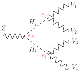
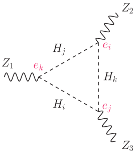
Figure 1: Feynman diagrams related to $\mbox{Im\thinspace}J_{2}$.

The amplitude of the left (tree level) diagrams (a total of six diagrams) will be proportional to

$${\cal M}\propto\sum_{i,j,k}\epsilon_{ijk}e_{i}e_{j}e_{k}\frac{1}{p_{34}^{2}-M_{i}^{2}}\frac{1}{p_{12}^{2}-M_{j}^{2}}$$ (4.1)

where $p_{12}$ is the sum of the momenta of $V_{1}$ and $V_{2}$, whereas $p_{34}$ is the sum of the momenta of $V_{3}$ and $V_{4}$. The pairs $V_{1}V_{2}$ and $V_{3}V_{4}$ may be either $ZZ$-pairs or $W^{+}W^{-}$-pairs. Performing the sum over all possible combinations of internal $H_{i}$ and $H_{j}$ and over $k$, we get

$${\cal M}\propto\frac{(p_{34}^{2}-p_{12}^{2})v^{9}\mbox{Im\thinspace}J_{2}}{\displaystyle\prod_{n=1}^{3}(p_{12}^{2}-M_{n}^{2})(p_{34}^{2}-M_{n}^{2})}.$$ (4.2)

The amplitude of the right (triangle loop) diagrams (six in total) will be proportional to

$${\cal M} \propto \sum_{i,j,k}\int d^{4}q\sum_{a,b,c}\epsilon_{ija}\epsilon_{kjb}\epsilon_{ikc}e_{a}e_{b}e_{c}\frac{1}{q^{2}-M_{i}^{2}}\frac{1}{(q+p_{1})^{2}-M_{j}^{2}}\frac{1}{(q+p_{1}+p_{2})^{2}-M_{k}^{2}}$$ (4.3)

$$\times(2q+p_{1})^{\mu_{1}}(2q+2p_{1}+p_{2})^{\mu_{2}}(2q+p_{1}+p_{2})^{\mu_{3}}$$

where $p_{1}$ and $p_{2}$ are the (incoming) momenta of $Z_{1}$ and $Z_{2}$, respectively. Performing the sum over $i,j,k$, we find

$${\cal M} \propto \int d^{4}q\frac{[q^{2}-(q+p_{1})^{2}][q^{2}-(q+p_{1}+p_{2})^{2}][(q+p_{1})^{2}-(q+p_{1}+p_{2})^{2}]v^{9}\mbox{Im\thinspace}J_{2}}{\displaystyle\prod_{n=1}^{3}(q^{2}-M_{n}^{2})((q+p_{1})^{2}-M_{n}^{2})((q+p_{1}+p_{2})^{2}-M_{n}^{2})}$$ (4.4)

$$\times(2q+p_{1})^{\mu_{1}}(2q+2p_{1}+p_{2})^{\mu_{2}}(2q+p_{1}+p_{2})^{\mu_{3}}.$$

We see from this that the amplitudes of both these diagrams are directly proportional to $\mbox{Im\thinspace}J_{2}$.

4.2 $\mbox{Im\thinspace}J_{1}$

Since $\mbox{Im\thinspace}J_{1}$ is bilinear in $e_{i}$ and linear in $q_{i}$, we look for Feynman diagrams containing three vertices, where two of the vertices are proportional to $e_{i}$, and the third vertex is an $H_{i}H^{+}H^{-}$-vertex. Also, since $\mbox{Im\thinspace}J_{1}$ contains the antisymmetric tensor $\epsilon_{ijk}$, we are led to choose one of the vertices to be $ZH_{i}H_{j}$. This leads us to a study of the Feynman amplitude structure shown in figure 2.

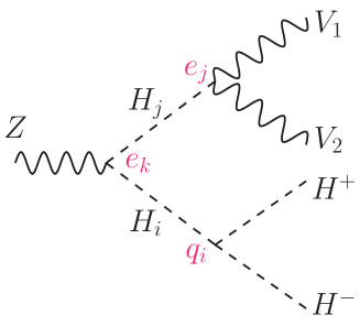
Figure 2: Feynman diagram related to $\mbox{Im\thinspace}J_{1}$.

The amplitude corresponding to the six diagrams shown in figure 2 is proportional to

$${\cal M}\propto\sum_{i,j,k}\epsilon_{ijk}q_{i}e_{j}e_{k}\frac{1}{p_{HH}^{2}-M_{i}^{2}}\frac{1}{p_{12}^{2}-M_{j}^{2}}$$ (4.5)

where $p_{12}$ is the sum of the momenta of $V_{1}$ and $V_{2}$, whereas $p_{HH}$ is the sum of the momenta of the $H^{+}H^{-}$-pair. The $V_{1}V_{2}$-pair may be either a $ZZ$-pair or a $W^{+}W^{-}$-pair. Summing over $i,j,k$, we get

$${\cal M}\propto\frac{C_{1}\mbox{Im\thinspace}J_{1}+C_{11}\mbox{Im\thinspace}J_{11}+C_{12}\mbox{Im\thinspace}J_{12}}{\displaystyle\prod_{n=1}^{3}(p_{12}^{2}-M_{n}^{2})(p_{HH}^{2}-M_{n}^{2})}$$ (4.6)

where

$$\mbox{Im\thinspace}J_{11} = \frac{1}{v^{7}}\sum_{i,j,k}\epsilon_{ijk}e_{i}M_{i}^{2}M_{j}^{2}e_{k}q_{j},$$ (4.7)

$$\mbox{Im\thinspace}J_{12} = \frac{1}{v^{9}}\sum_{i,j,k}\epsilon_{ijk}e_{i}M_{i}^{2}M_{j}^{4}e_{k}q_{j},$$ (4.8)

$$C_{1} = \left[p_{12}^{2}(p_{HH}^{2}-p_{12}^{2})(M_{1}^{2}+M_{2}^{2}+M_{3}^{2}-p_{12}^{2}-p_{HH}^{2})\right.$$ (4.9)

$$\left.-(p_{12}^{2}-M_{1}^{2})(p_{12}^{2}-M_{2}^{2})(p_{12}^{2}-M_{3}^{2})\right]v^{5},$$

$$C_{11} = \left[p_{HH}^{2}-(M_{1}^{2}+M_{2}^{2}+M_{3}^{2})\right](p_{HH}^{2}-p_{12}^{2})v^{7},$$ (4.10)

$$C_{12} = (p_{HH}^{2}-p_{12}^{2})v^{9}.$$ (4.11)

The quantities $\mbox{Im\thinspace}J_{11}$ and $\mbox{Im\thinspace}J_{12}$ are both bilinear in $e_{i}$ and linear in $q_{i}$, but have different “mass weights” compared to $\mbox{Im\thinspace}J_{1}$. Simple algebra shows that they both vanish when $\mbox{Im\thinspace}J_{1}=\mbox{Im\thinspace}J_{2}=0$.

Let us also note the intriguing property that as

$$p_{HH}^{2}\to p_{12}^{2},$$ (4.12)

then ${\cal M}$ simplifies enormously since $C_{11}=C_{12}=0$, and the total amplitude becomes proportional to $\mbox{Im\thinspace}J_{1}$. In principle, one could imagine exploiting this property experimentally by studying this process for a range of kinematical configurations, and extrapolating to the limit (4.12).

4.3 $\mbox{Im\thinspace}J_{30}$

Since $\mbox{Im\thinspace}J_{30}$ is linear in $e_{i}$ and bilinear in $q_{i}$, in this case we look for Feynman diagrams containing three vertices, where one vertex is proportional to $e_{i}$, and the two other vertices are $H_{i}H^{+}H^{-}$-vertices. In order to incorporate $\epsilon_{ijk}$ that is present in $\mbox{Im\thinspace}J_{30}$ we again choose one of the vertices to be $ZH_{i}H_{j}$. This leads us to a study of the Feynman amplitude structures shown in figure 3.

                 

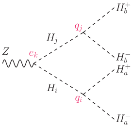
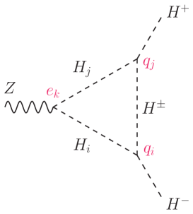
Figure 3: Feynman diagrams related to $\mbox{Im\thinspace}J_{30}$.

The amplitude of the six left (tree level) diagrams will be proportional to

$${\cal M}\propto\sum_{i,j,k}\epsilon_{ijk}q_{i}q_{j}e_{k}\frac{1}{p_{a}^{2}-M_{i}^{2}}\frac{1}{p_{b}^{2}-M_{j}^{2}}$$ (4.13)

where $p_{a}$ and $p_{b}$ denote the sum of the (outgoing) momenta of the $H_{a}^{-}H_{a}^{+}$ and $H_{b}^{-}H_{b}^{+}$ pairs, respectively. Summing over all possible combinations of $i,j,k$, we obtain

$${\cal M}\propto\frac{(p_{a}^{2}-p_{b}^{2})\left[p_{a}^{2}p_{b}^{2}v^{5}\mbox{Im\thinspace}J_{30}-(p_{a}^{2}+p_{b}^{2})v^{7}\mbox{Im\thinspace}J_{31}+v^{9}\mbox{Im\thinspace}J_{32}\right]}{\displaystyle\prod_{n=1}^{3}(p_{a}^{2}-M_{n}^{2})(p_{b}^{2}-M_{n}^{2})}.$$ (4.14)

Similarly, the amplitude of the six right (triangle loop) diagrams will be proportional to

$${\cal M} \propto \sum_{i,j,k}\int d^{4}q\epsilon_{ijk}q_{i}q_{j}e_{k}\frac{1}{q^{2}-M_{i}^{2}}\frac{1}{(q+p_{Z})^{2}-M_{j}^{2}}\frac{1}{(q+p_{Z}+p_{+})^{2}-M_{H^{\pm}}^{2}}$$ (4.15)

$$\times(2q+p_{Z})^{\mu}$$

where $p_{Z}$ and $p_{+}$ are the (incoming) momenta of $Z$ and $H^{+}$, respectively. Summing over all possible combinations of $i,j,k$ we find

$${\cal M} \propto \int d^{4}q\frac{q^{2}(q+p_{Z})^{2}v^{5}\mbox{Im\thinspace}J_{30}-[q^{2}+(q+p_{Z})^{2}]v^{7}\mbox{Im\thinspace}J_{31}+v^{9}\mbox{Im\thinspace}J_{32}}{\displaystyle[(q+p_{Z}+p_{+})^{2}-M_{H^{\pm}}^{2}]\prod_{n=1}^{3}(q^{2}-M_{n}^{2})((q+p_{Z})^{2}-M_{n}^{2})}$$ (4.16)

$$\times[q^{2}-(q+p_{Z})^{2}](2q+p_{Z})^{\mu}.$$

Here,

$$\mbox{Im\thinspace}J_{31} = \frac{1}{v^{7}}\sum_{i,j,k}\epsilon_{ijk}q_{i}M_{i}^{2}M_{j}^{2}e_{j}q_{k},$$ (4.17)

$$\mbox{Im\thinspace}J_{32} = \frac{1}{v^{9}}\sum_{i,j,k}\epsilon_{ijk}q_{i}M_{i}^{2}M_{j}^{4}e_{j}q_{k}.$$ (4.18)

The quantities $\mbox{Im\thinspace}J_{31}$ and $\mbox{Im\thinspace}J_{32}$ are both linear in $e_{i}$ and bilinear in $q_{i}$, but have different “mass weights” compared to $\mbox{Im\thinspace}J_{30}$. Simple algebra shows that they vanish when $\mbox{Im\thinspace}J_{1}=\mbox{Im\thinspace}J_{2}=\mbox{Im\thinspace}J_{30}=0$.

5 The alignment limit

As is well known, the properties of the Higgs boson discovered at the LHC are close to those predicted by the SM cms_coupl ; Aad:2014eha ; Aad:2014tca . Motivated by this experimental fact we shall in this section discuss the limit of the 2HDM which reproduces the SM couplings of $H_{1}$ to vector bosons. The limit is referred to as alignment, see sec. 1.3 in Asner:2013psa and Craig:2013hca ; Carena:2013ooa .

It should be emphasized that no assumptions concerning the mass spectrum of non-standard Higgs bosons is being made here. Therefore the alignment limit is not identical to the decoupling limit Gunion:2002zf which is defined by increasing the masses of non-standard Higgs bosons. Of course, decoupling implies alignment, but the inverse is not true. In fact, it has recently been verified Dumont:2014wha by fitting the 2HDM (type I and II) to available experimental data, that the model indeed allows for masses of extra scalars even within the $150-200$ GeV range, which is below the decoupling regime.

Within the CP-violating 2HDM the coupling of $H_{1}$ to a pair of vector bosons, $e_{1}$, can be written as:

$$e_{1}=v\cos(\alpha_{2})\cos(\alpha_{1}-\beta),$$ (5.1)

where $\tan\beta=v_{2}/v_{1}$. The alignment is equivalent to putting $e_{1}=v$. Since the $e_{i}$ satisfy the unitarity sum rule $\sum_{i=1,2,3}e_{i}^{2}=v^{2}$, alignment implies also $e_{2}=e_{3}=0$, meaning

$$\alpha_{1}=\beta,\quad\alpha_{2}=0.$$ (5.2)

The rotation matrix in this case becomes

$$R=\begin{pmatrix}R_{11}&R_{12}&R_{13}\\ R_{21}&R_{22}&R_{23}\\ R_{31}&R_{32}&R_{33}\end{pmatrix}=\begin{pmatrix}c_{\beta}&s_{\beta}&0\\ -s_{\beta}\,c_{3}&c_{\beta}\,c_{3}&s_{3}\\ s_{\beta}\,s_{3}&-c_{\beta}\,s_{3}&c_{3}\end{pmatrix}.$$ (5.3)

Note that the mixing matrix could be written in this case as

$$R=R_{3}R_{1}=\begin{pmatrix}1&0&0\\ 0&c_{3}&s_{3}\\ 0&-s_{3}&c_{3}\end{pmatrix}\begin{pmatrix}c_{\beta}&s_{\beta}&0\\ -s_{\beta}\ &c_{\beta}&0\\ 0&0&1\end{pmatrix}.$$ (5.4)

The couplings between $H_{i}$ and $H^{+}H^{-}$ simplify in the alignment limit:

$$q_{1} = \frac{1}{v}\left(2M_{H^{\pm}}^{2}-2\mu^{2}+M_{1}^{2}\right),$$ (5.5)

$$q_{2} = +c_{3}\left[\frac{(c_{\beta}^{2}-s_{\beta}^{2})}{vc_{\beta}s_{\beta}}(M_{2}^{2}-\mu^{2})+\frac{v}{2s_{\beta}^{2}}\mbox{Re\thinspace}\lambda_{6}-\frac{v}{2c_{\beta}^{2}}\mbox{Re\thinspace}\lambda_{7}\right]+s_{3}\frac{v}{2c_{\beta}s_{\beta}}\mbox{Im\thinspace}\lambda_{5},$$ (5.6)

$$q_{3} = -s_{3}\left[\frac{(c_{\beta}^{2}-s_{\beta}^{2})}{vc_{\beta}s_{\beta}}(M_{3}^{2}-\mu^{2})+\frac{v}{2s_{\beta}^{2}}\mbox{Re\thinspace}\lambda_{6}-\frac{v}{2c_{\beta}^{2}}\mbox{Re\thinspace}\lambda_{7}\right]+c_{3}\frac{v}{2c_{\beta}s_{\beta}}\mbox{Im\thinspace}\lambda_{5}.$$ (5.7)

It is easy to see that in this limit, the expressions for the CP-violating invariants become

$$\mbox{Im\thinspace}J_{1} = 0,$$

$$\mbox{Im\thinspace}J_{2} = 0,$$ (5.8)

$$\mbox{Im\thinspace}J_{30} = \frac{q_{2}q_{3}}{v^{4}}(M_{3}^{2}-M_{2}^{2}).$$

Two comments are here in order. First, note that $e_{1}=v$ implies no CP violation in the couplings to gauge bosons ($\mbox{Im\thinspace}J_{2}=0$), the only possible CP violation may appear in cubic scalar couplings $(H_{2}H^{+}H^{-})$ and $(H_{3}H^{+}H^{-})$, proportional to $q_{2}$ and $q_{3}$, respectively. Second, the necessary condition for CP violation is that both $(H_{2}H^{+}H^{-})$ and $(H_{3}H^{+}H^{-})$ couplings must exist together with a non-zero $ZH_{2}H_{3}$ vertex ($\propto e_{1}$). Note that the existence of the latter implies that for CP invariance, either $H_{2}$ or $H_{3}$ would have to be odd under CP. However, since they both couple to $H^{+}H^{-}$ (that is CP even), there would be no way to preserve CP.

It is important to note that in the case when $\lambda_{6}=\lambda_{7}=0$ (due to ${\mathbbm{Z}}_{2}$ symmetry imposed on the dimension-4 part of the potential) the $(1,3)$ and $(2,3)$ entries of the neutral mass-squared matrix, ${\cal M}^{2}_{13}$ and ${\cal M}^{2}_{23}$, are related as follows

$${\cal M}^{2}_{13}=t_{\beta}{\cal M}^{2}_{23},$$ (5.9)

where $t_{\beta}\equiv\tan\beta$. As a consequence of the above relation there is a constraint that relates mass eigenvalues, mixing angles and $t_{\beta}$ Khater:2003wq :

$$M_{1}^{2}R_{13}(R_{12}t_{\beta}-R_{11})+M_{2}^{2}R_{23}(R_{22}t_{\beta}-R_{21})+M_{3}^{2}R_{33}(R_{32}t_{\beta}-R_{31})=0.$$ (5.10)

In the alignment limit, the above relation simplifies to $(M_{2}^{2}-M_{3}^{2})s_{3}c_{3}s_{\beta}=0$, so that either $M_{2}=M_{3}$, $\alpha_{3}=0$ or $\alpha_{3}=\pm\pi/2$. It is easy to see that in all three cases, CP violation disappears. If $M_{2}=M_{3}$ then after the following reparametrization of $H_{i}$

$$\begin{pmatrix}H_{1}\\ H_{2}\\ H_{3}\end{pmatrix}\to R_{3}\begin{pmatrix}H_{1}\\ H_{2}\\ H_{3}\end{pmatrix},$$ (5.11)

the resulting mixing matrix is just $R=R_{1}$, implying no CP violation, consistent with $\mbox{Im\thinspace}J_{30}=0$. If, on the other hand, $\alpha_{3}=0$ or $\pm\pi/2$, then $q_{2}=0$ or $q_{3}=0$, respectively, so again $\mbox{Im\thinspace}J_{30}=0.$ It must be emphasized that the above important conclusion was based on the assumption that $\lambda_{6}=\lambda_{7}=0$.

If, on the other hand, $\lambda_{6}\neq 0$ and/or $\lambda_{7}\neq 0$, then ${\cal M}^{2}_{13}$ and ${\cal M}^{2}_{23}$ are not correlated as in (5.9), and we may not claim that $M_{2}=M_{3}$, nor that $\alpha_{3}=0$ or $\pm\pi/2$. So there is still room for CP violation.

Attempts to find symmetries that would naturally lead to alignment severely restrict the model. One possibility is just the standard ${\mathbbm{Z}}_{2}$ (invoked usually upon dimension-4 terms to suppress FCNC in Yukawa couplings) imposed in the Higgs basis, see sec. 1.3 in Asner:2013psa . This symmetry is however much too restrictive as it implies both $\lambda_{6}=0$ and $\lambda_{7}=0$ (possibly together with $m_{12}^{2}=0$), while the alignment comprises just one constraint i.e., $e_{1}=v$. Obviously, when the symmetry is imposed there is no way to accommodate CP violation in the scalar potential. Another attempt to find alignment was discussed recently in Dev:2014yca , where the authors introduce a 2HDM based on the SO(5) group and show that this leads to alignment. Dimension-4 terms in the scalar potential are assumed to be invariant under SO(5), while the symmetry is softly broken by bilinear Higgs mass terms. In addition the symmetry is violated by the hypercharge gauge coupling and third-generation Yukawa couplings. Again, the symmetry is so restrictive that there is no room for CP-violation in the scalar potential within this scenario.

So far, we have defined alignment in terms of mixing angles, $\alpha_{1}=\beta$ and $\alpha_{2}=0$. However, it is also worth trying to express the conditions in terms of the potential parameters. Especially, in the case of seeking a symmetry responsible for the alignment it is necessary to have the alignment condition in terms of scalar quartic coupling constants. Let us start with the relation between the initial, non-diagonal scalar mass-squared matrix ${\cal M}^{2}$ and the mixing angles. In general we have

$$R{\cal M}^{2}R^{\rm T}={\cal M}^{2}_{\rm diag}={\rm diag}(M_{1}^{2},M_{2}^{2},M_{3}^{2}).$$

In the case of alignment, $R=R_{3}R_{\beta}$ where $R_{\beta}\equiv R_{1}|_{\alpha_{1}=\beta}$. Then the mass-squared matrix ${\cal M}^{2}$ must be diagonalizable by $R_{3}R_{\beta}$. Therefore it is of the following form:

$${\cal M}^{2}=R_{\beta}^{T}R_{3}^{T}{\cal M}^{2}_{\rm diag}R_{3}R_{\beta}.$$ (5.12)

For a given $t_{\beta}$ the above form of ${\cal M}^{2}$ has 4 independent parameters, while in general it would have 6 parameters. Therefore we anticipate the existence of two relations between the a priori independent entries of ${\cal M}^{2}$. Those relations would be the wanted alignment conditions, expressed in terms of the potential parameters and $t_{\beta}$. Indeed, from (5.12) one can find the following constraints satisfied by the entries of ${\cal M}^{2}$:

$${\cal M}_{13}^{2} = -t_{\beta}{\cal M}_{23}^{2},$$ (5.13)

$$\left(t_{\beta}^{-1}-t_{\beta}\right){\cal M}_{12}^{2} = ({\cal M}_{11}^{2}-{\cal M}_{22}^{2}).$$ (5.14)

It is worth noting that these two formulas are satisfied not only by $e_{1}=v$, in fact they hold whenever $e_{i}^{2}=v^{2}$ for any $i=1,2,3$. Using the general formulae for the elements of ${\cal M}^{2}$, (A.5)–(A.10) one finds from (5.13)–(5.14)

$$v_{2}^{2}\mbox{Im\thinspace}\left(e^{i\xi}\lambda_{7}\right)+v_{2}v_{1}\mbox{Im\thinspace}\left(e^{2i\xi}\lambda_{5}\right)+v_{1}^{2}\mbox{Im\thinspace}\left(e^{i\xi}\lambda_{6}\right) = 0,$$ (5.15)

$$v_{2}^{4}\mbox{Re\thinspace}\left(e^{i\xi}\lambda_{7}\right)+v_{2}^{3}v_{1}(-\lambda_{2}+\lambda_{345})+3v_{2}^{2}v_{1}^{2}\mbox{Re\thinspace}\left[e^{i\xi}(\lambda_{6}-\lambda_{7})\right]+$$

$$+v_{2}v_{1}^{3}(\lambda_{1}-\lambda_{345})-v_{1}^{4}\mbox{Re\thinspace}\left(e^{i\xi}\lambda_{6}\right) = 0$$ (5.16)

where $\lambda_{345}\equiv\lambda_{3}+\lambda_{4}+\mbox{Re\thinspace}\left(e^{2i\xi}\lambda_{5}\right)$, and the terms have been ordered in powers of $v_{1}$ and $v_{2}$. In the CP-conserving limit, with $\xi=0$, $\mbox{Im\thinspace}\lambda_{5}=\mbox{Im\thinspace}\lambda_{6}=\mbox{Im\thinspace}\lambda_{7}=0$, we reproduce the single alignment condition found recently in ref. Dev:2014yca . If one wishes to satisfy the alignment conditions for any value of $v_{1}$, $v_{2}$ and $\xi$, then the following constraints must be fulfilled:

$$\lambda_{1}=\lambda_{2}=\lambda_{3}+\lambda_{4},\;\;\lambda_{5}=\lambda_{6}=\lambda_{7}=0.$$ (5.17)

Two comments are here in order. First, the above constraints eliminate the possibility of CP violation. Seeking a relation between quartic coupling constants that would be responsible for the alignment one would indeed have to satisfy (5.15)–(5.16) without any reference to the $v_{1}$, $v_{2}$ and $\xi$. Unfortunately its implication (5.17) is inconsistent with the possibility of having CP violated in the potential. However, the reader should be reminded that from a phenomenological point of view there is no need to satisfy the alignment conditions regardless of the value of $v_{2}/v_{1}$. We may conclude that for CP to be violated, $t_{\beta}$ must be properly tuned to satisfy the alignment conditions. Second, it is amusing to note that a potential satisfying the conditions (5.17) in a CP-conserving case, has been considered in Chankowski:2000an in a different context, namely that of finding a 2HDM that would automatically satisfy the $S,T,U$ constraints. An underlying symmetry has not been determined.

We can conclude that the observation of the SM-like Higgs boson at the LHC implies (within the 2HDM with ${\mathbbm{Z}}_{2}$ softly broken) vanishing CP violation in the scalar potential. Note that this conclusion could be realized either by large masses of the extra Higgs bosons (the decoupling regime, the case we are not discussing) or by alignment with relatively light extra Higgs bosons (the case discussed here). For both possibilities the $H_{1}VV$ coupling is SM-like so CP violation disappears within the 2HDM with softly broken ${\mathbbm{Z}}_{2}$ symmetry. We can summarize by emphasizing that, in order for CP violation to be present in the scalar potential, then the LHC data would favour a generic 2HDM with no ${\mathbbm{Z}}_{2}$ symmetry (thus allowing for non-zero $\lambda_{6}$ and/or $\lambda_{7}$). A consequence of that would be the interesting possibility of large (tree-level generated) FCNC in some Yukawa couplings.

6 Numerical illustrations

In reality measurements will never tell us that indeed the $H_{1}VV$ coupling is exactly SM-like, so we should allow for some maximal deviation from alignment. For that purpose we define

$$\delta\equiv 1-e_{1}/v$$ (6.1)

and illustrate predictions for the remaining CP violation as functions of $\delta$.

First we specify two cases of our scanning strategy.

• We denote by 2HDM5 the model with ${\mathbbm{Z}}_{2}$ softly broken, so $\lambda_{6}=\lambda_{7}=0$. The model parameters are listed as

  $${\cal P}_{5}\equiv\{M_{H^{\pm}}^{2},\mu^{2},M_{1}^{2},M_{2}^{2},v_{1},v_{2},\xi=0,\alpha_{1},\alpha_{2},\alpha_{3}\}.$$

  In this case we fix $M_{H^{\pm}}^{2}$, $\mu^{2}$, $M_{2}$, $\tan\beta$ (for the LHC Higgs boson we use $M_{1}=125\;\hbox{GeV}$) and scan over $-\pi/2\leq\alpha_{1},\alpha_{2},\alpha_{3}\leq\pi/2$ for chosen maximal deviation $\delta$, imposing $M_{1}<M_{2}<M_{3}$, vacuum stability and unitarity.

• 2HDM67 refers to the general 2HDM, so that ${\mathbbm{Z}}_{2}$ is not imposed, consequently $\lambda_{6}\neq 0,\lambda_{7}\neq 0$. In this case the parameters of the model are

  $${\cal P}_{67}\equiv\{M_{H^{\pm}}^{2},\mu^{2},M_{1}^{2},M_{2}^{2},M_{3}^{2},{\rm Im}\lambda_{5},{\rm Re}\lambda_{6},{\rm Re}\lambda_{7},v_{1},v_{2},\xi=0,\alpha_{1},\alpha_{2},\alpha_{3}\}$$

  For this general case $M_{H^{\pm}}^{2}$, $\mu^{2}$, $M_{2}$, $M_{3}$, and $\tan\beta$ are fixed (for the LHC Higgs boson we use $M_{1}=125\;\hbox{GeV}$) while we scan over $-\pi/2\leq\alpha_{1},\alpha_{2},\alpha_{3}\leq\pi/2$ and $|{\rm Im}\lambda_{5}|,|{\rm Re}\lambda_{6}|,|{\rm Re}\lambda_{7}|<5$, for chosen maximal deviation $\delta$, imposing $M_{1}<M_{2}<M_{3}$, vacuum stability and unitarity.

Figure 4 illustrates regions of $(\alpha_{1},\alpha_{2})$ (see Eq. (5.2)) which are compatible with $\delta\leq 0.05$, the external edge corresponds to $\delta=0.05$. Approaching the center of the contours $\delta\to 0$.

In figures 5–7 we show correlations between $\mbox{Im\thinspace}J_{i}$ and $\delta$. As one could have anticipated from the discussion of alignment, all the invariants must vanish as $\delta$ decreases in the model with $\lambda_{6}=\lambda_{7}=0$. However, as seen in Fig. 7, when $\lambda_{6}\neq 0$ and/or $\lambda_{7}\neq 0$ then $\mbox{Im\thinspace}J_{30}$ does not vanish even when $\delta\to 0$, as illustrated by the green dots for small values of $\delta$, corresponding to non-zero $\mbox{Im\thinspace}J_{30}$. Typically $\mbox{Im\thinspace}J_{30}\sim 1-3$, showing a large amount of CP violation present in the model even in the vicinity of the alignment limit.

Before closing this section let us focus on the figure showing $\mbox{Im\thinspace}J_{2}$, where remarkably the green dots are all inside a triangular region with a clear boundary. In order to understand this, we recall that

$$\mbox{Im\thinspace}J_{2} = \frac{2e_{1}e_{2}e_{3}}{v^{9}}(M_{1}^{2}-M_{2}^{2})(M_{2}^{2}-M_{3}^{2})(M_{3}^{2}-M_{1}^{2})$$

Using the fact that $e_{1}=v(1-\delta)$ and $|e_{3}|=\sqrt{v^{2}-e_{1}^{2}-e_{2}^{2}}$, one can easily find that for small $\delta$, $|\mbox{Im\thinspace}J_{2}|_{\rm max}$ simplifies to a linear function reproducing the triangle shape

$$|\mbox{Im\thinspace}J_{2}|_{\rm max} \simeq \frac{\delta}{v^{6}}(M_{1}^{2}-M_{2}^{2})(M_{2}^{2}-M_{3}^{2})(M_{3}^{2}-M_{1}^{2}).$$ (6.2)

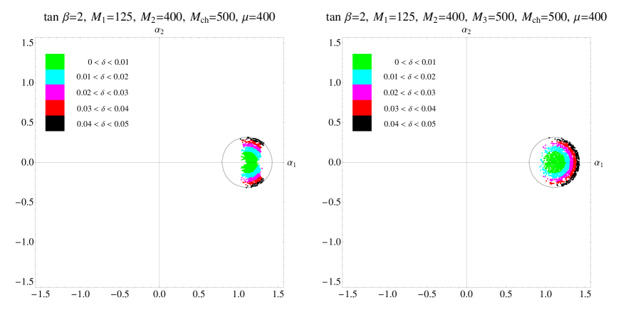
Figure 4: Allowed regions in the $(\alpha_{1},\alpha_{2})$ space for $\tan\beta=2$ corresponding to maximal deviation $\delta=0.05$ within the 2HDM5 (${\mathbbm{Z}}_{2}$ softly broken) and 2HDM67, are shown in the left and right panels, respectively. The coloring corresponds to ranges of $\delta$ shown in the legend. Vacuum stability and unitarity constraints are satisfied. The parameters adopted are $M_{1}=125$ GeV, $M_{2}=400$ GeV, $M_{H^{\pm}}=500$ GeV, $\tan\beta=2$, $\mu=400$ GeV for the 2HDM5. For the 2HDM67, in addition, $M_{3}=500$ GeV.

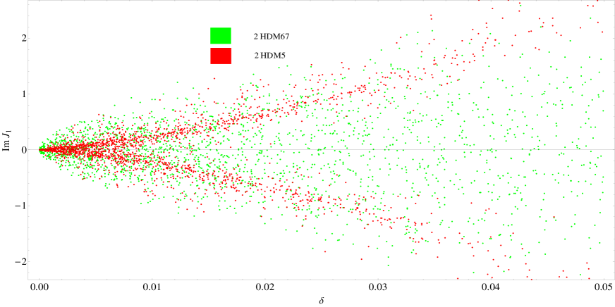
Figure 5: Correlation between $\mbox{Im\thinspace}J_{1}$ and the deviation $\delta$ for $\delta\leq 0.05$. Green and red dots correspond to 2HDM67 and 2HDM5, respectively.

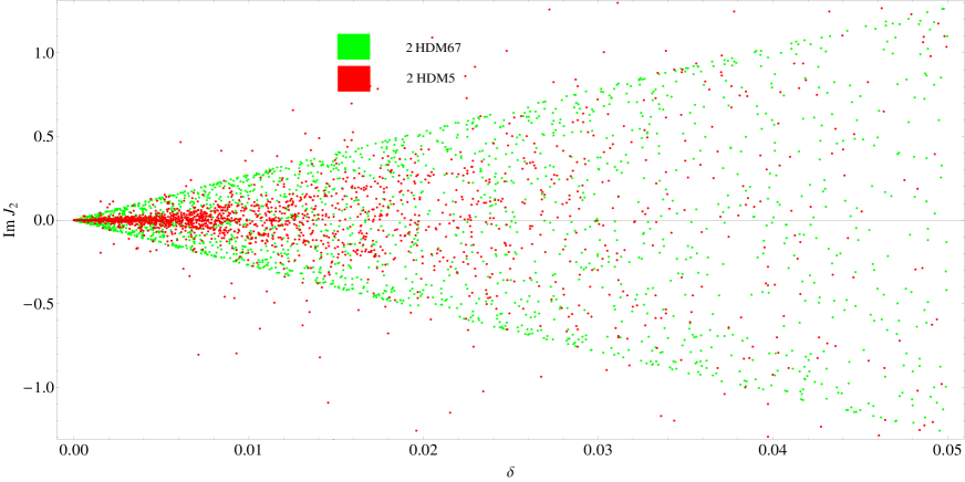
Figure 6: Correlation between $\mbox{Im\thinspace}J_{2}$ and the deviation $\delta$ for $\delta\leq 0.05$. Green and red dots correspond to 2HDM67 and 2HDM5, respectively.

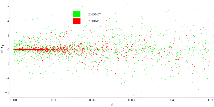
Figure 7: Correlation between $\mbox{Im\thinspace}J_{30}$ and the deviation $\delta$ for $\delta\leq 0.05$. Green and red dots correspond to 2HDM67 and 2HDM5, respectively.

7 Search strategy

We have identified processes related to all the $\mbox{Im\thinspace}J_{i}$, so that now we are able to propose a strategy to test if all the $\mbox{Im\thinspace}J_{i}$ vanish (implying CP conservation), or if one of them is nonzero (CP violation). Since in the alignment limit only $\mbox{Im\thinspace}J_{30}$ might be non-vanishing we focus on prospects for its measurement.

Step 1: Let us start with $\mbox{Im\thinspace}J_{2}$, and choose one of the processes shown in figure 1. The triangle-loop diagram to the right is more appealing due to the fact that the $ZZZ$-vertex is absent at tree-level. As we have shown, the amplitude is directly proportional to $\mbox{Im\thinspace}J_{2}$, and is thus suitable to determine whether $\mbox{Im\thinspace}J_{2}$ vanishes or not.

Phenomenological discussions Hagiwara:1986vm ; Gounaris:2000dn ; Baur:2000ae of the $ZZZ$ vertex have presented its most general Lorentz structure. In Ref. Gounaris:2000dn the CP-violating vertex is analyzed, with $Z_{1},Z_{2},Z_{3}$ all off-shell. A total of 14 Lorentz structures are identified, all preserving parity. Some of these vanish when one or more $Z$ is on-shell. If we characterize them by momenta and Lorentz indices ($p_{1},\mu_{1}$), ($p_{2},\mu_{2}$) and ($p_{3},\mu_{3}$), and let $Z_{2}$ and $Z_{3}$ be on-shell, then the structure reduces to the form

$$e\Gamma_{ZZZ}^{\mu_{1}\mu_{2}\mu_{3}}=ief_{4}^{Z}\frac{p_{1}^{2}-M_{Z}^{2}}{M_{Z}^{2}}(p_{1}^{\mu_{2}}g^{\mu_{1}\mu_{3}}+p_{1}^{\mu_{3}}g^{\mu_{1}\mu_{2}}),$$ (7.1)

where $e$ is the proton charge and $f_{4}^{Z}$ is a dimensionless form factor. This structure arises from an effective CP-violating operator of the form Gounaris2:2000

$${\cal O}_{ZZZ}=\frac{-e}{m_{Z}^{2}}f_{4}^{Z}\left[\partial_{\mu}\left(\partial^{\mu}Z^{\beta}-\partial^{\beta}Z^{\mu}\right)\right]Z_{\alpha}\left(\partial^{\alpha}Z_{\beta}\right).$$ (7.2)

A more detailed phenomenological discussion of $f_{4}^{Z}$ will be presented elsewhere GOO .

Step 2: If in Step 1 we have been able to determine a nonzero $\mbox{Im\thinspace}J_{2}$, then we know that the 2HDM violates CP. If, on the other hand, we find that $\mbox{Im\thinspace}J_{2}$ is consistent with zero, then the next step would be to proceed to $\mbox{Im\thinspace}J_{1}$, in order to determine if this quantity vanishes or not. For the process shown in figure 2, we have already shown that in the case of $\mbox{Im\thinspace}J_{2}=0$, the amplitude will vanish if $\mbox{Im\thinspace}J_{1}$ vanishes. We choose $V_{1}V_{2}$ to be a $W^{+}W^{-}$-pair since it makes all particles involved distinguishable. Characterizing $Z,W^{-}$ and $W^{+}$ by Lorentz indices $\mu_{1}$, $\mu_{2}$ and $\mu_{3}$, respectively, the Lorentz-structure for this process is proportional to

$$(p_{VV}-p_{HH})^{\mu_{1}}g^{\mu_{2}\mu_{3}}=(p_{Z}-2p_{HH})^{\mu_{1}}g^{\mu_{2}\mu_{3}}.$$ (7.3)

The effective Lagrangian giving rise to such a structure would be

$$\left[(\partial_{\mu}Z^{\mu})H^{+}H^{-}-2Z^{\mu}(H^{-}\partial_{\mu}H^{+}+H^{+}\partial_{\mu}H^{-})\right]W_{\alpha}^{\dagger}W^{\alpha},$$ (7.4)

which also clearly violates CP. Again, it is beyond the scope of this work to discuss further phenomenological consequences of this amplitude.
Step 3: If we by now have confirmed that both $\mbox{Im\thinspace}J_{1}$ and $\mbox{Im\thinspace}J_{2}$ vanish, the only possibility for a CP-violating 2HDM would be if $\mbox{Im\thinspace}J_{30}$ were nonzero, so we turn to the processes in figure 3. Of these processes, the triangle-loop diagram is more appealing due to fewer particles in the “final” state. The Lorentz structure for this process will consist of two parts:

$$Ap_{Z}^{\mu}+B(p_{+}-p_{-})^{\mu}.$$ (7.5)

Here, $A$ will be a CP-violating form factor, and $B$ will be a CP-conserving form factor. The effective Lagrangian giving rise to the CP-violating part would be

$${\cal O}_{ZH^{+}H^{-}}^{CPV}=Z_{\mu}\left[(\partial^{\mu}H^{+})H^{-}+(\partial^{\mu}H^{-})H^{+}\right],$$ (7.6)

and for the CP conserving one

$${\cal O}_{ZH^{+}H^{-}}^{CPC}=Z_{\mu}\left[(\partial^{\mu}H^{+})H^{-}-(\partial^{\mu}H^{-})H^{+}\right].$$ (7.7)

At the tree-level, the contribution to the $ZH^{+}H^{-}$-vertex is proportional to $(p_{+}-p_{-})^{\mu}$, which is CP-conserving. CP-violating contributions (proportional to $p_{Z}^{\mu}$) arise only at loop level. In experiment, we would need to single out the parts proportional to $p_{Z}^{\mu}$ in order to measure whether $\mbox{Im\thinspace}J_{30}$ vanishes or not. In the SM, $A$ (arising from the CKM matrix) would also be generated via quark loops, however a non vanishing contribution requires at least a 3-loop diagram, so it is efficiently suppressed.

8 Summary

In this paper we have expressed the three invariants $\mbox{Im\thinspace}J_{i}$ in terms of physically observable quantities like couplings and masses, independently confirming the result of Lavoura:1994fv ; Botella:1994cs . We have used this to formulate conditions for CP conservation in terms of couplings and masses. We have also identified processes that are sensitive to each of the $\mbox{Im\thinspace}J_{i}$, in order to figure out how to determine, through experiment, whether the 2HDM is CP violating or not.

We have further investigated the scenario in which the lightest neutral scalar mimics the SM Higgs boson, showing that there is still room for CP violation, provided we have nonzero $\lambda_{6}$ and/or $\lambda_{7}$, i.e., non-conserved ${\mathbbm{Z}}_{2}$ symmetry.

We have also found that there is a conflict between the possibility of violating CP in the potential and explanation of the alignment by relations (perhaps symmetry) satisfied by the quartic coupling constants in the scalar potential for any $v_{1}$, $v_{2}$ and the relative phase $\xi$.

Bearing in mind the Higgs LHC data, we have sketched a strategy that may lead to an experimental test of CP violation in the scalar sector of the 2HDM. A detailed experimental study of $ZZZ$ and $ZH^{+}H^{-}$ vertices together with $Z^{\star}\to VVH^{+}H^{-}$ seem to be necessary in order to test CP symmetry in the scalar potential. The proposed strategy would certainly constitute a very serious experimental challenge, but a result would be highly significant.

Appendix A Further properties of the model

In this appendix we collect formulas relevant for minimization of the potential and determination of scalar masses. We also show relations between quartic coupling constants and masses and mixing angles, they are crucial to show that potential parameters could indeed be expressed through the parameter set (3.2) that we are adopting. It should be emphasized that the relations presented here are applicable for the most general 2HDM without any ${\mathbbm{Z}}_{2}$ symmetry imposed on the model.

A.1 Stationary points of the potential

By demanding that the derivatives of the potential (2) with respect to the fields should vanish in the vacuum, we end up with the following stationary-point equations:

$$m_{11}^{2} = v_{1}^{2}\lambda_{1}+v_{2}^{2}(\lambda_{3}+\lambda_{4})+\frac{v_{2}^{2}}{c_{\xi}}(\mbox{Re\thinspace}\lambda_{5}c_{\xi}-\mbox{Im\thinspace}\lambda_{5}s_{\xi})$$ (A.1)

$$+\frac{v_{1}v_{2}}{c_{\xi}}\left[\mbox{Re\thinspace}\lambda_{6}(2+c_{2\xi})-\mbox{Im\thinspace}\lambda_{6}s_{2\xi}\right]+\frac{v_{2}}{v_{1}c_{\xi}}(v_{2}^{2}\mbox{Re\thinspace}\lambda_{7}-\mbox{Re\thinspace}m_{12}^{2}),$$

$$m_{22}^{2} = v_{2}^{2}\lambda_{2}+v_{1}^{2}(\lambda_{3}+\lambda_{4})+\frac{v_{1}^{2}}{c_{\xi}}(\mbox{Re\thinspace}\lambda_{5}c_{\xi}-\mbox{Im\thinspace}\lambda_{5}s_{\xi})$$ (A.2)

$$+\frac{v_{1}v_{2}}{c_{\xi}}\left[\mbox{Re\thinspace}\lambda_{7}(2+c_{2\xi})-\mbox{Im\thinspace}\lambda_{7}s_{2\xi}\right]+\frac{v_{1}}{v_{2}c_{\xi}}(v_{1}^{2}\mbox{Re\thinspace}\lambda_{6}-\mbox{Re\thinspace}m_{12}^{2}),$$

$$\mbox{Im\thinspace}m_{12}^{2} = \frac{v_{1}v_{2}}{c_{\xi}}(\mbox{Re\thinspace}\lambda_{5}s_{2\xi}+\mbox{Im\thinspace}\lambda_{5}c_{2\xi})+\frac{v_{1}^{2}}{c_{\xi}}(\mbox{Re\thinspace}\lambda_{6}s_{\xi}+\mbox{Im\thinspace}\lambda_{6}c_{\xi})$$ (A.3)

$$+\frac{v_{2}^{2}}{c_{\xi}}(\mbox{Re\thinspace}\lambda_{7}s_{\xi}+\mbox{Im\thinspace}\lambda_{7}c_{\xi})-\mbox{Re\thinspace}m_{12}^{2}t_{\xi},$$

with $c_{x}=\cos x$, $s_{x}=\sin x$, and $t_{x}=\tan x$. Thus, we may eliminate $m_{11}^{2}$, $m_{22}^{2}$ and $\mbox{Im\thinspace}m_{12}^{2}$ from the potential by these substitutions, thereby reducing the number of parameters of the model.

A.2 The scalar masses and the re-expression of the $\lambda$s

From the bilinear terms of potential, we may read off directly the mass of the charged scalars

$$M_{H^{\pm}}^{2}=\frac{v^{2}}{2v_{1}v_{2}c_{\xi}}\mbox{Re\thinspace}\left(m_{12}^{2}-v_{1}^{2}\lambda_{6}-v_{2}^{2}\lambda_{7}-v_{1}v_{2}e^{i\xi}\left[\lambda_{4}+\lambda_{5}\right]\right),$$ (A.4)

and the elements of the neutral-sector mass matrix

$${\cal M}_{11}^{2} = v_{1}^{2}\lambda_{1}-v_{2}^{2}s^{2}_{\xi}\mbox{Re\thinspace}\lambda_{5}-\frac{v_{2}^{2}}{2c_{\xi}}s_{\xi}c_{2\xi}\mbox{Im\thinspace}\lambda_{5}+\frac{v_{1}v_{2}}{2c_{\xi}}(1+2c_{2\xi})\mbox{Re\thinspace}\lambda_{6}$$ (A.5)

$$-2v_{1}v_{2}s_{\xi}\mbox{Im\thinspace}\lambda_{6}-\frac{v_{2}^{3}}{2v_{1}c_{\xi}}\mbox{Re\thinspace}\lambda_{7}+\frac{v_{2}}{2v_{1}c_{\xi}}\mbox{Re\thinspace}m_{12}^{2},$$

$${\cal M}_{22}^{2} = v_{2}^{2}\lambda_{2}-v_{1}^{2}s^{2}_{\xi}\mbox{Re\thinspace}\lambda_{5}-\frac{v_{1}^{2}}{2c_{\xi}}s_{\xi}c_{2\xi}\mbox{Im\thinspace}\lambda_{5}+\frac{v_{1}v_{2}}{2c_{\xi}}(1+2c_{2\xi})\mbox{Re\thinspace}\lambda_{7}$$ (A.6)

$$-2v_{1}v_{2}s_{\xi}\mbox{Im\thinspace}\lambda_{7}-\frac{v_{1}^{3}}{2v_{2}c_{\xi}}\mbox{Re\thinspace}\lambda_{6}+\frac{v_{1}}{2v_{2}c_{\xi}}\mbox{Re\thinspace}m_{12}^{2},$$

$${\cal M}_{33}^{2} = -v^{2}c^{2}_{\xi}\mbox{Re\thinspace}\lambda_{5}-\frac{v^{2}}{2c_{\xi}}(2s^{3}_{\xi}-3s_{\xi})\mbox{Im\thinspace}\lambda_{5}$$ (A.7)

$$-\frac{v^{2}v_{1}}{2v_{2}c_{\xi}}\mbox{Re\thinspace}\lambda_{6}-\frac{v^{2}v_{2}}{2v_{1}c_{\xi}}\mbox{Re\thinspace}\lambda_{7}+\frac{v^{2}}{2v_{1}v_{2}c_{\xi}}\mbox{Re\thinspace}m_{12}^{2},$$

$${\cal M}_{12}^{2} = v_{1}v_{2}(\lambda_{3}+\lambda_{4})+v_{1}v_{2}c^{2}_{\xi}\mbox{Re\thinspace}\lambda_{5}+\frac{v_{1}v_{2}}{2c_{\xi}}(2s^{3}_{\xi}-3s_{\xi})\mbox{Im\thinspace}\lambda_{5}+\frac{v_{1}^{2}}{2c_{\xi}}(2+c_{2\xi})\mbox{Re\thinspace}\lambda_{6}$$ (A.8)

$$-v_{1}^{2}s_{\xi}\mbox{Im\thinspace}\lambda_{6}+\frac{v_{2}^{2}}{2c_{\xi}}(2+c_{2\xi})\mbox{Re\thinspace}\lambda_{7}-v_{2}^{2}s_{\xi}\mbox{Im\thinspace}\lambda_{7}-\frac{1}{2c_{\xi}}\mbox{Re\thinspace}m_{12}^{2},$$

$${\cal M}_{13}^{2} = -{\textstyle\frac{1}{2}}vv_{2}s_{2\xi}\mbox{Re\thinspace}\lambda_{5}-{\textstyle\frac{1}{2}}vv_{2}c_{2\xi}\mbox{Im\thinspace}\lambda_{5}-vv_{1}s_{\xi}\mbox{Re\thinspace}\lambda_{6}-vv_{1}c_{\xi}\mbox{Im\thinspace}\lambda_{6},$$ (A.9)

$${\cal M}_{23}^{2} = -{\textstyle\frac{1}{2}}vv_{1}s_{2\xi}\mbox{Re\thinspace}\lambda_{5}-{\textstyle\frac{1}{2}}vv_{1}c_{2\xi}\mbox{Im\thinspace}\lambda_{5}-vv_{2}s_{\xi}\mbox{Re\thinspace}\lambda_{7}-vv_{2}c_{\xi}\mbox{Im\thinspace}\lambda_{7}.$$ (A.10)

The eigenvalues of this matrix will be the masses of the three neutral scalars. In order to find these, a cubic equation needs to be solved. For our purposes, a different approach will suffice. We may rewrite the elements of the mass matrix ${\cal M}_{ij}^{2}$ in terms of the eigenvalues $M_{i}^{2}$ and elements of the rotation matrix $R_{ij}$ as six equations:

$${\cal M}_{11}^{2} = M_{1}^{2}R_{11}^{2}+M_{2}^{2}R_{21}^{2}+M_{3}^{2}R_{31}^{2},$$ (A.11)

$${\cal M}_{22}^{2} = M_{1}^{2}R_{12}^{2}+M_{2}^{2}R_{22}^{2}+M_{3}^{2}R_{32}^{2},$$ (A.12)

$${\cal M}_{33}^{2} = M_{1}^{2}R_{13}^{2}+M_{2}^{2}R_{23}^{2}+M_{3}^{2}R_{33}^{2},$$ (A.13)

$${\cal M}_{12}^{2} = M_{1}^{2}R_{11}R_{12}+M_{2}^{2}R_{21}R_{22}+M_{3}^{2}R_{31}R_{32},$$ (A.14)

$${\cal M}_{13}^{2} = M_{1}^{2}R_{11}R_{13}+M_{2}^{2}R_{21}R_{23}+M_{3}^{2}R_{31}R_{33},$$ (A.15)

$${\cal M}_{23}^{2} = M_{1}^{2}R_{12}R_{13}+M_{2}^{2}R_{22}R_{23}+M_{3}^{2}R_{32}R_{33}.$$ (A.16)

We may now regard (A.4) and (A.11)–(A.16) as a set of seven equations. These equations are linear in the $\lambda_{i}$-parameters of the potential. We have 10 such parameters (counting both real and imaginary parts of $\lambda_{5}$, $\lambda_{6}$ and $\lambda_{7}$) and may now solve this set of seven equations for seven of the $\lambda_{i}$-parameters, thus expressing them in terms of the other parameters we have introduced. It is convenient to solve for the following set of parameters: $(\lambda_{1},\lambda_{2},\lambda_{3},\lambda_{4},{\rm Re}\lambda_{5},{\rm Im}\lambda_{6},{\rm Im}\lambda_{7})$. We also introduce the more convenient parameter $\mu^{2}$ by putting

$${\rm Re}\hskip 2.84544ptm_{12}^{2}=\frac{2v_{1}v_{2}}{v^{2}}\mu^{2}.$$ (A.17)

Solving the set of equations, we arrive at

$$\lambda_{1} = -\frac{v_{2}^{2}}{v^{2}v_{1}^{2}c_{\xi}^{3}}\mu^{2}+\frac{\left(R_{11}v-R_{13}v_{2}t_{\xi}\right)^{2}}{v^{2}v_{1}^{2}}M_{1}^{2}+\frac{\left(R_{21}v-R_{23}v_{2}t_{\xi}\right)^{2}}{v^{2}v_{1}^{2}}M_{2}^{2}$$ (A.18)

$$+\frac{\left(R_{31}v-R_{33}v_{2}t_{\xi}\right)^{2}}{v^{2}v_{1}^{2}}M_{3}^{2}-\frac{v_{2}^{2}t_{\xi}}{2v_{1}^{2}c_{\xi}^{2}}{\rm Im}\lambda_{5}$$

$$-\frac{v_{2}(2c_{2\xi}+1)}{2v_{1}c_{\xi}^{3}}{\rm Re}\lambda_{6}+\frac{v_{2}^{3}}{2v_{1}^{3}c_{\xi}^{3}}{\rm Re}\lambda_{7},$$

$$\lambda_{2} = -\frac{v_{1}^{2}}{v^{2}v_{2}^{2}c_{\xi}^{3}}\mu^{2}+\frac{\left(R_{12}v-R_{13}v_{1}t_{\xi}\right)^{2}}{v^{2}v_{2}^{2}}M_{1}^{2}+\frac{\left(R_{22}v-R_{23}v_{1}t_{\xi}\right)^{2}}{v^{2}v_{2}^{2}}M_{2}^{2}$$ (A.19)

$$+\frac{\left(R_{32}v-R_{33}v_{1}t_{\xi}\right)^{2}}{v^{2}v_{2}^{2}}M_{3}^{2}-\frac{v_{1}^{2}t_{\xi}}{2v_{2}^{2}c_{\xi}^{2}}{\rm Im}\lambda_{5}$$

$$+\frac{v_{1}^{3}}{2v_{2}^{3}c_{\xi}^{3}}{\rm Re}\lambda_{6}-\frac{v_{1}(2c_{2\xi}+1)}{2v_{2}c_{\xi}^{3}}{\rm Re}\lambda_{7},$$

$$\lambda_{3} = \frac{2}{v^{2}}M_{H^{\pm}}^{2}-\frac{1}{v^{2}c_{\xi}^{3}}\mu^{2}+\frac{\left(R_{12}v-R_{13}v_{1}t_{\xi}\right)\left(R_{11}v-R_{13}v_{2}t_{\xi}\right)}{v^{2}v_{1}v_{2}}M_{1}^{2}$$ (A.20)

$$+\frac{\left(R_{22}v-R_{23}v_{1}t_{\xi}\right)\left(R_{21}v-R_{23}v_{2}t_{\xi}\right)}{v^{2}v_{1}v_{2}}M_{2}^{2}$$

$$+\frac{\left(R_{32}v-R_{33}v_{1}t_{\xi}\right)\left(R_{31}v-R_{33}v_{2}t_{\xi}\right)}{v^{2}v_{1}v_{2}}M_{3}^{2}$$

$$-\frac{1}{2c_{\xi}^{2}}t_{\xi}{\rm Im}\lambda_{5}-\frac{v_{1}c_{2\xi}}{2v_{2}c_{\xi}^{3}}{\rm Re}\lambda_{6}-\frac{v_{2}c_{2\xi}}{2v_{1}c_{\xi}^{3}}{\rm Re}\lambda_{7},$$

$$\lambda_{4} = -\frac{2}{v^{2}}M_{H^{\pm}}^{2}+\frac{c_{2\xi}}{v^{2}c_{\xi}^{3}}\mu^{2}+\frac{R_{13}^{2}}{v^{2}c_{\xi}^{2}}M_{1}^{2}+\frac{R_{23}^{2}}{v^{2}c_{\xi}^{2}}M_{2}^{2}+\frac{R_{33}^{2}}{v^{2}c_{\xi}^{2}}M_{3}^{2}$$ (A.21)

$$-\frac{1}{2c_{\xi}^{2}}t_{\xi}{\rm Im}\lambda_{5}-\frac{v_{1}c_{2\xi}}{2v_{2}c_{\xi}^{3}}{\rm Re}\lambda_{6}-\frac{v_{2}c_{2\xi}}{2v_{1}c_{\xi}^{3}}{\rm Re}\lambda_{7},$$

$${\rm Re}\lambda_{5} = \frac{1}{v^{2}c_{\xi}^{3}}\mu^{2}-\frac{R_{13}^{2}}{v^{2}c_{\xi}^{2}}M_{1}^{2}-\frac{R_{23}^{2}}{v^{2}c_{\xi}^{2}}M_{2}^{2}-\frac{R_{33}^{2}}{v^{2}c_{\xi}^{2}}M_{3}^{2}$$ (A.22)

$$+\frac{1}{4c_{\xi}^{3}}(3s_{\xi}+s_{3\xi}){\rm Im}\lambda_{5}-\frac{v_{1}}{2v_{2}c_{\xi}^{3}}{\rm Re}\lambda_{6}-\frac{v_{2}}{2v_{1}c_{\xi}^{3}}{\rm Re}\lambda_{7},$$

$${\rm Im}\lambda_{6} = -\frac{v_{2}t_{\xi}}{v^{2}v_{1}c_{\xi}^{2}}\mu^{2}+\frac{R_{13}\left(R_{13}v_{2}t_{\xi}-R_{11}v\right)}{v^{2}v_{1}c_{\xi}}M_{1}^{2}+\frac{R_{23}\left(R_{23}v_{2}t_{\xi}-R_{21}v\right)}{v^{2}v_{1}c_{\xi}}M_{2}^{2}$$

$$+\frac{R_{33}\left(R_{33}v_{2}t_{\xi}-R_{31}v\right)}{v^{2}v_{1}c_{\xi}}M_{3}^{2}-\frac{v_{2}}{2v_{1}c_{\xi}^{3}}{\rm Im}\lambda_{5}-\frac{1}{2c_{\xi}^{2}}t_{\xi}c_{2\xi}{\rm Re}\lambda_{6}+\frac{v_{2}^{2}t_{\xi}}{2v_{1}^{2}c_{\xi}^{2}}{\rm Re}\lambda_{7},$$

$${\rm Im}\lambda_{7} = -\frac{v_{1}t_{\xi}}{v^{2}v_{2}c_{\xi}^{2}}\mu^{2}+\frac{R_{13}\left(R_{13}v_{1}t_{\xi}-R_{12}v\right)}{v^{2}v_{2}c_{\xi}}M_{1}^{2}+\frac{R_{23}\left(R_{23}v_{1}t_{\xi}-R_{22}v\right)}{v^{2}v_{2}c_{\xi}}M_{2}^{2}$$

$$+\frac{R_{33}\left(R_{33}v_{1}t_{\xi}-R_{32}v\right)}{v^{2}v_{2}c_{\xi}}M_{3}^{2}-\frac{v_{1}}{2v_{2}c_{\xi}^{3}}{\rm Im}\lambda_{5}+\frac{v_{1}^{2}t_{\xi}}{2v_{2}^{2}c_{\xi}^{2}}{\rm Re}\lambda_{6}-\frac{1}{2c_{\xi}^{2}}t_{\xi}c_{2\xi}{\rm Re}\lambda_{7}.$$

These substitutions enable us to express quantities (couplings, observables, etc.) arising from the vevs and the potential in terms of the set of parameters ${\cal P}_{67}$ of equation (3.2). We also note that each of the seven expressions listed above is linear in the subset of parameters denoted ${\cal P}_{0}$ and given by equation (3.3).

Appendix B Relevant coupling coefficients

The couplings involving scalars can be read off from the relevant parts of the Lagrangian, and hence the Feynman rules for different interactions can be found. We shall here present expressions for the couplings relevant for the bosonic sector of the model. Some of them were not adopted explicitly in the main text, however we find it useful to collect them here for completeness and future reference. The couplings involving physical scalars only are quite lengthy, so we will introduce the following abbreviations in order to compactify them:

$$e_{i} \equiv v_{1}R_{i1}+v_{2}R_{i2},$$ (B.1)

$$f_{i} \equiv v_{1}R_{i2}-v_{2}R_{i1}-ivR_{i3},$$ (B.2)

$$g_{i} \equiv v_{1}^{3}R_{i2}+v_{2}^{3}R_{i1},$$ (B.3)

$$h_{iik} \equiv v_{1}R_{i2}^{2}R_{k2}+v_{2}R_{i1}^{2}R_{k1}.$$ (B.4)

B.1 The $H_{i}H^{-}H^{+}$, $H_{i}H_{i}H^{-}H^{+}$ and $H^{-}H^{-}H^{+}H^{+}$ couplings

In addition to containing terms bilinear in the fields (that give us the masses of the scalar particles), the potential also contains trilinear and quadrilinear terms corresponding to interactions between the fields. In the present work, we shall need the $H_{i}H^{-}H^{+}$, $H_{i}H_{i}H^{-}H^{+}$ and $H^{-}H^{-}H^{+}H^{+}$ couplings. Reading the coefficients of these interactions directly off from the potential, we find

$$q_{i} \equiv \text{Coefficient}(V,H_{i}H^{-}H^{+})$$ (B.5)

$$= \frac{2e_{i}}{v^{2}}M_{H^{\pm}}^{2}-\frac{R_{i2}v_{1}+R_{i1}v_{2}-R_{i3}vt_{\xi}}{v_{1}v_{2}c_{\xi}}\mu^{2}+\frac{g_{i}-R_{i3}v^{3}t_{\xi}}{v^{2}v_{1}v_{2}}M_{i}^{2}+\frac{R_{i3}v^{3}}{2v_{1}v_{2}c_{\xi}^{2}}\mbox{Im\thinspace}\lambda_{5}$$

$$-\frac{v^{2}\left(R_{i3}vt_{\xi}-R_{i2}v_{1}+R_{i1}v_{2}\right)}{2v_{2}^{2}c_{\xi}}\mbox{Re\thinspace}\lambda_{6}-\frac{v^{2}\left(R_{i3}vt_{\xi}+R_{i2}v_{1}-R_{i1}v_{2}\right)}{2v_{1}^{2}c_{\xi}}\mbox{Re\thinspace}\lambda_{7},$$

$$q_{ii} \equiv \text{Coefficient}(V,H_{i}H_{i}H^{-}H^{+})$$ (B.6)

$$= \frac{e_{i}^{2}}{v^{4}}M_{H^{\pm}}^{2}-\frac{\left(v_{1}^{2}-v_{2}^{2}\right)^{2}|f_{i}|^{2}+2v_{1}v_{2}e_{i}g_{i}-2v^{3}v_{1}v_{2}e_{i}R_{i3}t_{\xi}+v^{4}|f_{i}|^{2}t_{\xi}^{2}}{2v^{4}v_{1}^{2}v_{2}^{2}c_{\xi}}\mu^{2}$$

$$+\frac{1}{2v^{4}v_{1}^{2}v_{2}^{2}}\sum_{k=1}^{3}\left[g_{k}\left(2e_{i}R_{i3}R_{k3}v_{1}v_{2}+g_{k}R_{i3}^{2}+h_{iik}v^{2}\right)\right.$$

$$\hskip 85.35826pt-vR_{k3}\left(g_{k}\left(|f_{i}|^{2}+R_{i3}^{2}v^{2}\right)+2e_{i}R_{i3}R_{k3}v_{1}v_{2}v^{2}+h_{iik}v^{4}\right)t_{\xi}$$

$$\hskip 85.35826pt\left.+|f_{i}|^{2}R_{k3}^{2}v^{4}t_{\xi}^{2}\right]M_{k}^{2}$$

$$+\frac{2e_{i}R_{i3}vv_{1}v_{2}-v^{2}|f_{i}|^{2}t_{\xi}}{4v_{1}^{2}v_{2}^{2}c_{\xi}^{2}}\mbox{Im\thinspace}\lambda_{5}$$

$$+\frac{1}{4v_{1}v_{2}^{3}c_{\xi}}\left[v^{2}\left(R_{i3}^{2}\left(v_{1}^{2}-v_{2}^{2}\right)+R_{i2}^{2}v_{1}^{2}-R_{i1}^{2}v_{2}^{2}\right)-2|f_{i}|^{2}v_{2}^{2}\right.$$

$$\hskip 56.9055pt\left.-2e_{i}R_{i3}vv_{1}v_{2}t_{\xi}+|f_{i}|^{2}v^{2}t_{\xi}^{2}\right]\mbox{Re\thinspace}\lambda_{6}$$

$$+\frac{1}{4v_{2}v_{1}^{3}c_{\xi}}\left[-v^{2}\left(R_{i3}^{2}\left(v_{1}^{2}-v_{2}^{2}\right)+R_{i2}^{2}v_{1}^{2}-R_{i1}^{2}v_{2}^{2}\right)-2|f_{i}|^{2}v_{1}^{2}\right.$$

$$\hskip 56.9055pt\left.-2e_{i}R_{i3}vv_{1}v_{2}t_{\xi}+v^{2}|f_{i}|^{2}t_{\xi}^{2}\right]\mbox{Re\thinspace}\lambda_{7},$$

$$q \equiv \text{Coefficient}(V,H^{-}H^{-}H^{+}H^{+})$$ (B.7)

$$= -\frac{1}{2v^{2}v_{1}^{2}v_{2}^{2}c_{\xi}}\left[\left(v_{1}^{2}-v_{2}^{2}\right)^{2}+v^{4}t_{\xi}^{2}\right]\mu^{2}+\sum_{k=1}^{3}\frac{\left(g_{k}-R_{k3}v^{3}t_{\xi}\right)^{2}}{2v^{4}v_{1}^{2}v_{2}^{2}}M_{k}^{2}-\frac{v^{4}t_{\xi}}{4v_{1}^{2}v_{2}^{2}c_{\xi}^{2}}\mbox{Im\thinspace}\lambda_{5}$$

$$+\frac{v^{2}\left(v_{1}^{2}-3v_{2}^{2}+v^{2}t_{\xi}^{2}\right)}{4v_{1}v_{2}^{3}c_{\xi}}\mbox{Re\thinspace}\lambda_{6}+\frac{v^{2}\left(v_{2}^{2}-3v_{1}^{2}+v^{2}t_{\xi}^{2}\right)}{4v_{2}v_{1}^{3}c_{\xi}}\mbox{Re\thinspace}\lambda_{7}.$$

An important property of these couplings is that they are linear in the parameters of the set ${\cal P}_{0}$. It is also worth pointing out that these couplings are not identical to the Feynman rules for the interactions they represent. One needs to take into account the fact that the potential appears with a negative sign in the Lagrangian as well as the fact that combinatorial factors arising from the presence of multiple identical particles, and the imaginary unit $i$ should be present in the interactions terms. The corresponding Feynman rules become

$$H_{i}H^{+}H^{-}: -iq_{i},$$ (B.8)

$$H_{i}H_{i}H^{+}H^{-} -2iq_{ii},$$ (B.9)

$$H^{+}H^{+}H^{-}H^{-} -4iq.$$ (B.10)

There are many interesting and useful relations among the couplings of the model. We will point out a couple of these, but first let us introduce a quantity that is completely symmetric under the interchange of any two of the indices $1,2,3$:

$$\sigma\equiv q_{11}+q_{22}+q_{22}.$$ (B.11)

One can now easily show that

$$e_{i}q_{i}=(\sigma-q)e_{i}^{2}+(q_{ii}-q)v^{2},$$ (B.12)

which in turn leads to

$$e_{1}q_{1}+e_{2}q_{2}+e_{3}q_{3}=2(\sigma-2q)v^{2},$$ (B.13)

where we have used the fact that $e_{1}^{2}+e_{2}^{2}+e_{3}^{2}=v^{2}$.

B.2 Couplings containing the factor $e_{i}$

The quantity $e_{i}=v_{1}R_{i1}+v_{2}R_{i2}$ plays an important role as it appears as a factor in numerous interactions involving neutral scalars. Here, we list them in two groups, those that contain the antisymmetric $\epsilon_{ijk}$, and those that do not:

$$H_{i}H_{j}Z_{\mu}:\quad\frac{g}{2v\cos{\theta}_{\text{W}}}\epsilon_{ijk}e_{k}(p_{i}-p_{j})_{\mu},\quad H_{i}H_{j}G_{0}:\quad i\frac{M_{i}^{2}-M_{j}^{2}}{v^{2}}\epsilon_{ijk}e_{k},$$ (B.14)

and

$$H_{i}Z_{\mu}Z_{\nu}:\quad \frac{ig^{2}}{2\cos^{2}{\theta}_{\text{W}}}e_{i}\,g_{\mu\nu}, \quad H_{i}W^{+}_{\mu}W^{-}_{\nu}:\quad \frac{ig^{2}}{2}e_{i}\,g_{\mu\nu},$$ (B.15a)

$$H_{i}G_{0}G_{0}:\quad \frac{-iM_{i}^{2}e_{i}}{v^{2}}, \quad H_{i}G^{+}G^{-}:\quad \frac{-iM_{i}^{2}e_{i}}{v^{2}},$$ (B.15b)

$$H_{i}G^{+}A_{\mu}W^{-}_{\nu}:\quad \frac{ig^{2}\sin{\theta}_{\text{W}}}{2v}e_{i}\,g_{\mu\nu}, \quad H_{i}G^{-}A_{\mu}W^{+}_{\nu}:\quad \frac{ig^{2}\sin{\theta}_{\text{W}}}{2v}e_{i}\,g_{\mu\nu},$$ (B.15c)

$$H_{i}G^{+}Z_{\mu}W^{-}_{\nu}:\quad -\frac{ig^{2}}{2v}\frac{\sin^{2}{\theta}_{\text{W}}}{\cos{\theta}_{\text{W}}}e_{i}\,g_{\mu\nu}, \quad H_{i}G^{-}Z_{\mu}W^{+}_{\nu}:\quad -\frac{ig^{2}}{2v}\frac{\sin^{2}\theta_{\text{W}}}{\cos{\theta}_{\text{W}}}e_{i}\,g_{\mu\nu},$$ (B.15d)

$$H_{i}G_{0}Z_{\mu}:\quad \frac{g}{2v\cos{\theta}_{\text{W}}}e_{i}(p_{i}-p_{0})_{\mu},$$ (B.15e)

$$H_{i}G^{+}W^{-}_{\mu}:\quad i\frac{g}{2v}e_{i}(p_{i}-p^{+})_{\mu}, \quad H_{i}G^{-}W^{+}_{\mu}:\quad -i\frac{g}{2v}e_{i}(p_{i}-p^{-})_{\mu}.$$ (B.15f)

Here, $G_{0}$ and $G^{\pm}$ denote the Goldstone fields. Since the couplings (B.14) are the only ones that contain the antisymmetric $\epsilon_{ijk}$, one of these vertices must be involved in each of the invariants $\mbox{Im\thinspace}J_{1}$, $\mbox{Im\thinspace}J_{2}$, and $\mbox{Im\thinspace}J_{30}$.

In the notation of Accomando:2006ga ; El_Kaffas:2006nt , the different values can be expressed as

$$e_{1} =v\cos\alpha_{2}\cos(\beta-\alpha_{1}),$$ (B.16a)

$$e_{2} =v[\cos\alpha_{3}\sin(\beta-\alpha_{1})-\sin\alpha_{2}\sin\alpha_{3}\cos(\beta-\alpha_{1})],$$ (B.16b)

$$e_{3} =-v[\sin\alpha_{3}\sin(\beta-\alpha_{1})+\sin\alpha_{2}\cos\alpha_{3}\cos(\beta-\alpha_{1})].$$ (B.16c)

In the limits of CP conservation that are not a consequence of mass degeneracy ElKaffas:2007rq , one of the $e_{i}$ will vanish. For the 2HDM5, they are given as:

$$H_{1} =A: \quad e_{1} =0, \quad e_{2} =v\sin(\beta-\alpha_{1}\mp\alpha_{3}), \quad e_{3} =\mp v\cos(\beta-\alpha_{1}\mp\alpha_{3}),$$ (B.17a)

$$H_{2} =A: \quad e_{1} =v\cos(\beta-\alpha_{1}), \quad e_{2} =0, \quad e_{3} =-v\sin(\beta-\alpha_{1}),$$ (B.17b)

$$H_{3} =A: \quad e_{1} =v\cos(\beta-\alpha_{1}), \quad e_{2} =v\sin(\beta-\alpha_{1}), \quad e_{3} =0,$$ (B.17c)

with $A$ here denoting the CP-odd neutral Higgs boson (not the photon). Substituting the mixing angle $\alpha$ describing the CP-conserving case, $\alpha_{1}=\alpha+\pi/2$, we recover the familiar $H_{1}ZZ$ and $H_{1}W^{+}W^{-}$ couplings (see Eq. (B.15a)) proportional to $e_{1}=v\sin(\beta-\alpha)$, valid when $H_{2}$ or $H_{3}$ is odd under $CP$.

We note that

$$e_{1}^{2}+e_{2}^{2}+e_{3}^{2}=v^{2}.$$ (B.18)

Clearly, equipartition maximizes the product $e_{1}e_{2}e_{3}$ which enters in $\mbox{Im\thinspace}J_{2}$. Thus

$$\max\frac{e_{1}e_{2}e_{3}}{v^{3}}=\frac{1}{3\sqrt{3}}\simeq 0.1925.$$ (B.19)

B.3 The coupling $q_{i}$

The trilinear neutral-charged Higgs coupling is denoted as $q_{i}$:

$$H_{i}H^{+}H^{-}:\quad-iq_{i}.$$ (B.20)

This coupling is more complicated than $e_{i}$ and $f_{i}$, when expressed in terms of the neutral-sector mixing matrix.

In the model discussed in Grzadkowski:2013rza , the coupling coefficient $q_{i}$ takes the form

$$H_{i}H^{+}H^{-}:\quad -iq_{i}$$ (B.21)

$$= -i\biggl{[}2M_{H^{\pm}}^{2}\frac{v_{1}R_{i1}+v_{2}R_{i2}}{v^{2}}-\mu^{2}\frac{v_{1}R_{i2}+v_{2}R_{i1}}{v_{1}v_{2}}+M_{i}^{2}\frac{v_{1}^{3}R_{i2}+v_{2}^{3}R_{i1}}{v_{1}v_{2}v^{2}}+\Delta\frac{vR_{i3}}{v_{1}v_{2}}\biggr{]}.$$

Here, $\Delta$ can be written as $\Delta\equiv v\Delta_{123}$, with

$$\Delta_{ijk}=\frac{(M_{k}^{2}-M_{j}^{2})R_{j3}R_{k3}}{v_{1}R_{i1}-v_{2}R_{i2}}.$$ (B.22)

B.4 The coupling $f_{i}$

Another coefficient appearing in many bosonic couplings is denoted $f_{i}$,

$$f_{i}\equiv v_{1}R_{i2}-v_{2}R_{i1}-ivR_{i3}.$$ (B.23)

In contrast to the $e_{i}$ (and $q_{i}$) it is complex. However, we note that they are related to the $e_{i}$ as follows:

$$\mbox{Re\thinspace}f_{i}f_{j}^{\ast}=v^{2}\delta_{ij}-e_{i}e_{j}.$$ (B.24)

$$H_{i}G^{-}H^{+}:\quad -i\frac{M_{i}^{2}-M_{H^{\pm}}^{2}}{v^{2}}f_{i}, \quad H_{i}G^{+}H^{-}:\quad -i\frac{M_{i}^{2}-M_{H^{\pm}}^{2}}{v^{2}}f_{i}^{\ast},$$ (B.25a)

$$H_{i}H^{+}A_{\mu}W^{-\mu}:\quad i\frac{g^{2}}{2v}\sin{\theta}_{\text{W}}f_{i}, \quad H_{i}H^{-}A_{\mu}W^{+\mu}:\quad i\frac{g^{2}}{2v}\sin{\theta}_{\text{W}}f_{i}^{\ast},$$ (B.25b)

$$H_{i}H^{+}Z_{\mu}W^{-\mu}:\quad \frac{-ig^{2}}{2v}\frac{\sin^{2}{\theta}_{\text{W}}}{\cos{\theta}_{\text{W}}}f_{i}, \quad H_{i}H^{-}Z_{\mu}W^{+\mu}:\quad \frac{-ig^{2}}{2v}\frac{\sin^{2}{\theta}_{\text{W}}}{\cos{\theta}_{\text{W}}}f_{i}^{\ast},$$ (B.25c)

$$H_{i}H^{-}W^{+\mu}:\quad \frac{ig}{2v}f_{i}(p_{i}-p^{-})^{\mu}, \quad H_{i}H^{+}W^{-\mu}:\quad \frac{-ig}{2v}f_{i}^{\ast}(p_{i}-p^{+})^{\mu}.$$ (B.25d)

In the CP-conserving limit, two of the $f_{i}$ are real, whereas the third is pure imaginary.

We note that the following relation follows from the unitarity of the rotation matrix:

$$\sum_{i,j,k}\epsilon_{ijk}e_{i}f_{j}^{\ast}f_{k}=-2iv^{3}.$$ (B.26)

References

- (1) A. Riotto and M. Trodden, Recent progress in baryogenesis, Ann. Rev. Nucl. Part. Sci. 49 (1999) 35 [hep-ph/9901362].
- (2) G. C. Branco, P. M. Ferreira, L. Lavoura, M. N. Rebelo, M. Sher and J. P. Silva, Theory and phenomenology of two-Higgs-doublet models, Phys. Rept. 516 (2012) 1 [arXiv:1106.0034 [hep-ph]].
- (3) L. Lavoura and J. P. Silva, Fundamental CP violating quantities in a SU(2) U(1) model with many Higgs doublets, Phys. Rev. D 50 (1994) 4619 [hep-ph/9404276].
- (4) F. J. Botella and J. P. Silva, Jarlskog-like invariants for theories with scalars and fermions, Phys. Rev. D 51 (1995) 3870 [hep-ph/9411288].
- (5) G. C. Branco, M. N. Rebelo and J. I. Silva-Marcos, CP-odd invariants in models with several Higgs doublets, Phys. Lett. B 614, 187 (2005) [hep-ph/0502118].
- (6) J. F. Gunion and H. E. Haber, Conditions for CP-violation in the general two-Higgs-doublet model, Phys. Rev. D 72 (2005) 095002 [hep-ph/0506227].
- (7) H. E. Haber and D. O’Neil, Phys. Rev. D 74, 015018 (2006) [hep-ph/0602242].
- (8) S. Davidson and H. E. Haber, Basis-independent methods for the two-Higgs-doublet model, Phys. Rev. D 72 (2005) 035004 [Erratum-ibid. D 72 (2005) 099902] [hep-ph/0504050].
- (9) I. P. Ivanov, Two-Higgs-doublet model from the group-theoretic perspective, Phys. Lett. B 632 (2006) 360 [hep-ph/0507132].
- (10) C. C. Nishi, CP violation conditions in N-Higgs-doublet potentials, Phys. Rev. D 74 (2006) 036003 [Erratum-ibid. D 76 (2007) 119901] [hep-ph/0605153].
- (11) I. P. Ivanov, Minkowski space structure of the Higgs potential in 2HDM, Phys. Rev. D 75 (2007) 035001 [Erratum-ibid. D 76 (2007) 039902] [hep-ph/0609018].
- (12) M. Maniatis, A. von Manteuffel and O. Nachtmann, CP violation in the general two-Higgs-doublet model: A Geometric view, Eur. Phys. J. C 57 (2008) 719 [arXiv:0707.3344 [hep-ph]].
- (13) G. C. Branco, L. Lavoura and J. P. Silva, CP Violation, Int. Ser. Monogr. Phys. 103, 1 (1999).
- (14) C. Jarlskog, Commutator of the Quark Mass Matrices in the Standard Electroweak Model and a Measure of Maximal CP Violation, Phys. Rev. Lett. 55 (1985) 1039.
- (15) G. Aad et al. [ATLAS Collaboration], Observation of a new particle in the search for the Standard Model Higgs boson with the ATLAS detector at the LHC, Phys. Lett. B 716 (2012) 1 [arXiv:1207.7214 [hep-ex]].
- (16) S. Chatrchyan et al. [CMS Collaboration], Observation of a new boson at a mass of 125 GeV with the CMS experiment at the LHC, Phys. Lett. B 716 (2012) 30 [arXiv:1207.7235 [hep-ex]].
- (17) E. Accomando, A. G. Akeroyd, E. Akhmetzyanova, J. Albert, A. Alves, N. Amapane, M. Aoki and G. Azuelos et al., Workshop on CP Studies and Non-Standard Higgs Physics, hep-ph/0608079.
- (18) A. W. El Kaffas, W. Khater, O. M. Ogreid and P. Osland, Consistency of the two Higgs doublet model and CP violation in top production at the LHC, Nucl. Phys. B 775 (2007) 45 [hep-ph/0605142].
- (19) T. D. Lee, A Theory of Spontaneous T Violation, Phys. Rev. D 8 (1973) 1226.
- (20) B. Grzadkowski, O. M. Ogreid and P. Osland, Diagnosing CP properties of the 2HDM, JHEP 1401 (2014) 105 [arXiv:1309.6229 [hep-ph], arXiv:1309.6229].
- (21) http://www.wolfram.com/mathematica/
- (22) CMS Collaboration, Precise determination of the mass of the Higgs boson and studies of the compatibility of its couplings with the standard model, Report number CMS-PAS-HIG-14-009.
- (23) G. Aad et al. [ATLAS Collaboration], Measurement of Higgs boson production in the diphoton decay channel in collisions at center-of-mass energies of 7 and 8 TeV with the ATLAS detector, arXiv:1408.7084 [hep-ex].
- (24) G. Aad et al. [ATLAS Collaboration], Fiducial and differential cross sections of Higgs boson production measured in the four-lepton decay channel in collisions at =8 TeV with the ATLAS detector, arXiv:1408.3226 [hep-ex].
- (25) D. M. Asner, T. Barklow, C. Calancha, K. Fujii, N. Graf, H. E. Haber, A. Ishikawa and S. Kanemura et al., ILC Higgs White Paper, arXiv:1310.0763 [hep-ph].
- (26) N. Craig, J. Galloway and S. Thomas, Searching for Signs of the Second Higgs Doublet, arXiv:1305.2424 [hep-ph].
- (27) M. Carena, I. Low, N. R. Shah and C. E. M. Wagner, Impersonating the Standard Model Higgs Boson: Alignment without Decoupling, JHEP 1404, 015 (2014) [arXiv:1310.2248 [hep-ph]].
- (28) J. F. Gunion and H. E. Haber, The CP conserving two Higgs doublet model: The Approach to the decoupling limit, Phys. Rev. D 67, 075019 (2003) [hep-ph/0207010].
- (29) B. Dumont, J. F. Gunion, Y. Jiang and S. Kraml, Constraints on and future prospects for Two-Higgs-Doublet Models in light of the LHC Higgs signal, Phys. Rev. D 90, 035021 (2014) [arXiv:1405.3584 [hep-ph]].
- (30) A. Barroso, P. M. Ferreira, R. Santos and J. P. Silva, Probing the scalar-pseudoscalar mixing in the 125 GeV Higgs particle with current data, Phys. Rev. D 86, 015022 (2012) [arXiv:1205.4247 [hep-ph]].
- (31) W. Khater and P. Osland, CP violation in top quark production at the LHC and two Higgs doublet models, Nucl. Phys. B 661, 209 (2003) [hep-ph/0302004].
- (32) P. S. B. Dev and A. Pilaftsis, arXiv:1408.3405 [hep-ph].
- (33) P. H. Chankowski, T. Farris, B. Grzadkowski, J. F. Gunion, J. Kalinowski and M. Krawczyk, Phys. Lett. B 496, 195 (2000) [hep-ph/0009271].
- (34) K. Hagiwara, R. D. Peccei, D. Zeppenfeld and K. Hikasa, Probing the Weak Boson Sector in , Nucl. Phys. B 282 (1987) 253.
- (35) G. J. Gounaris, J. Layssac and F. M. Renard, Off-shell structure of the anomalous and selfcouplings, Phys. Rev. D 62 (2000) 073012 [hep-ph/0005269].
- (36) U. Baur and D. L. Rainwater, Probing neutral gauge boson selfinteractions in production at hadron colliders, Phys. Rev. D 62 (2000) 113011 [hep-ph/0008063].
- (37) G. J. Gounaris, J. Layssac and F. M. Renard, Signatures of the anomalous and production at lepton and hadron colliders, Phys. Rev. D 61 (2000) 0730012 [hep-ph/9910395].
- (38) B. Grzadkowski, O. M. Ogreid and P. Osland, CP violating and vertices in the Two-Higgs-Doublet Model, to be published.
- (39) A. W. El Kaffas, P. Osland and O. M. Ogreid, CP violation, stability and unitarity of the two Higgs doublet model, Nonlin. Phenom. Complex Syst. 10 (2007) 347 [hep-ph/0702097].