Reactive Programming for Interactive Graphics

Abstract

One of the big challenges of developing interactive statistical applications is the management of the data pipeline, which controls transformations from data to plot. The user’s interactions needs to be propagated through these modules and reflected in the output representation at a fast pace. Each individual module may be easy to develop and manage, but the dependency structure can be quite challenging. The MVC (Model/View/Controller) pattern is an attempt to solve the problem by separating the user’s interaction from the representation of the data. In this paper we discuss the paradigm of reactive programming in the framework of the MVC architecture and show its applicability to interactive graphics. Under this paradigm, developers benefit from the separation of user interaction from the graphical representation, which makes it easier for users and developers to extend interactive applications. We show the central role of reactive data objects in an interactive graphics system, implemented as the R package cranvas, which is freely available on GitHub and the main developers include the authors of this paper.

, and

1 Introduction

Interactive graphics progresses us beyond the limitations of static statistical displays, in particular, for exploring multidimensional data. With a static image, we can only see one aspect of the data at a time. Interactive graphics allows us to inspect data dynamically from multiple views. For example, we may draw a scatterplot of two variables and a stacked bar chart showing the proportions of missing values for the rest of the variables in a data set (two stacked bars per variable). Then we can highlight the bar that indicates the missing values of one variable, and the subset of points corresponding to these missing values in the scatterplot are highlighted immediately, so we can examine the conditional bivariate relationship in the scatterplot.

The term “interactive graphics” can be ambiguous, as disclosed by Swayne and Klinke (1999) in an editorial of Computational Statistics: it may imply the direct manipulation of the graph itself, manipulation of the graph controls or even the command-line interaction with graphs. We primarily mean the direct manipulation on graphs, but other meanings still have their usefulness. For instance, we may change the bin width of a histogram through a slider or brush all the outliers in a scatterplot using a command line with a numeric criterion, achieving a higher degree of control than direct manipulation allows.

The main tasks that an interactive statistical graphics system should support are as follows: [2.]

Single display interactions, such as modifying the plot attributes (brushing, zooming, panning, deletion) and obtaining additional information (querying graphical elements);

Linking between different displays of the same data set or related data sets. For example, suppose we have a scatterplot of the variable $Y$ versus $X$ and a histogram of $Z$ (all three variables are from the same data set), when we highlight a subset of points in the scatterplot and we need to show the distribution of the subset of $Z$ in the histogram as well.

The first set of tasks is easier to solve—there are a lot of web applications that allow various single display interactions, for instance, Gapminder (Rosling and Johansson, 2009), ManyEyes (Viegas et al., 2007), JMP (SAS Institute, 2009) and D3 (Bostock, Ogievetsky and Heer, 2011).

Linked graphics, which is less common, allows changes across different displays as well as across different aggregation levels of the data. The key difficulty is how to let the plots be aware of each other’s changes and respond both automatically and immediately. There are several types of linking between plots, one-to-one linking, categorical linking and geographical linking (Dykes, 1998); see Hurley and Oldford (1988), Stuetzle (1987) and McDonald, Stuetzle and Buja (1990) for some early demonstrations and implementations. We will show how linking is related to, and achieved by, reactive programming in this paper.

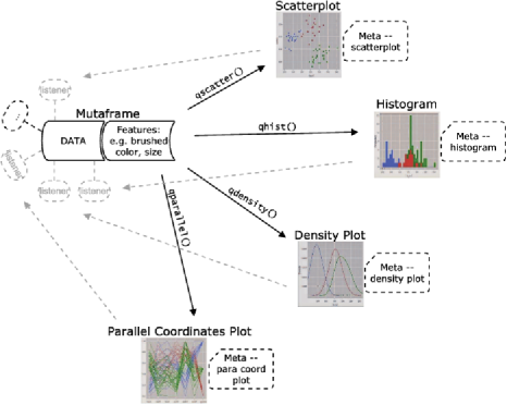
Figure 1: A representation of the pipeline in the cranvas package. It shows how plots are linked to each other as well as to the data source. Elements are added to the data to facilitate the interaction. Arrows with solid lines indicate R functions that draw the plots. Dashed lines indicate reactions fed back to the data elements.

A number of stand-alone systems for interactive statistical graphics exist. Early systems include PRIM-9, an interactive computer graphics system to picture, rotate, isolate and mask data in up to 9 dimensions (Fisherkeller, Friedman and Tukey, 1988). Data Desk (Velleman and Velleman, 1988) and LISP-STAT (Tierney, 1990) provided tight integration with interactive graphics as well as numerical modeling. In particular, LISP-STAT is also a programmable environment like R (R Core Team, 2013), but, unfortunately, today R is the more popular choice. Tierney (2005) described a few desirable approaches toward programmable interactive graphics, which were not implemented in LISP-STAT due to limitations of the toolkit. These are all relatively straightforward in the framework of R and Qt (Qt Project, 2013). XGobi and GGobi (Swayne et al. (2003); Cook and Swayne (2007)), MANET (Unwin et al., 1996) and Mondrian (Theus, 2002) support interactive displays of multivariate data, but lack extensibility and a tight integration with modeling in R. The rggobi package (Wickham et al., 2008) is an interface between R and GGobi based on the GTK+ toolkit. The iplots package (Urbanek and Wichtrey, 2013) provides high interaction statistical graphics; it is written in Java using the Swing toolkit and communicates with R through the rJava package.

One of the big challenges in the development of interactive statistical applications is to resolve a user’s action on the data level. This is sometimes referred to as the “plumbing” of interactive graphics. Buja et al. (1988, page 298) introduced the concept of a viewing pipeline for data plots. The pipeline takes the raw data, through transformation, standardization, randomization, projection, viewporting and graphical element in a plot. Some components of the pipeline can be made implicit, such as the so-called “window-to-viewport” transformation (i.e., viewporting), due to technological advances in computer graphics toolkits. For example, Qt can take care of such low-level details automatically. Wickham et al. (2009) outlined a more general pipeline for interactive graphics, but it did not cover implementation details, which is the focus of this paper.

The R package cranvas (Xie et al., 2013) is an interactive graphics system built under the classical Model/View/Controller (MVC) architecture and adopts the reactive programming paradigm to achieve interactivity. Figure 1 shows a basic pipeline in the cranvas package and its most important components, mutaframes and metadata objects, which are “reactive” by design. The pipeline starts with a data source (a mutaframe) as the central commander of the system. Any plot can modify the data source as the user interacts with the plot and, as soon as the mutaframe is modified, its reactive nature will propagate the changes to all other plots in the system automatically. In addition, each plot also has its own attributes that are described by the metadata beyond the mutaframes. A metadata object is also reactive, but it is only linked to a specific plot. For example, the bin width of a histogram is stored in its metadata, and when the user’s action induces a change in this value, the histogram responds accordingly.

The paper is organized as follows. We start with a discussion of the MVC design. Section 3 describes the reactive programming paradigm relative to the MVC architecture, using cranvas as an example. Section 4 provides specific examples of how interaction is realized.

2 The MVC Architecture

MVC is a software architecture design described originally by Trygve Reenskaug in the 1970s and in detail by Krasner and Pope (1988). It is widely used in GUI (Graphical User Interface) applications, including web applications (Leff and Rayfield, 2001). There have been a number of R packages utilizing the MVC architecture. For example, Whalen (2005) built an interactive GUI system using the MVC design to explore linked data. The GUI was based on the RGtk package, which later evolved into RGtk2 (Lawrence and Temple Lang, 2010), and MVC was implemented in the MVCClass package.

The main reason for the popularity of MVC is because it minimizes the dependencies between different components of an application. For example, let us assume that the model component consists of a data transformation, such as a square-root or log transformation. The model does not depend on the view, but the view depends on the model in the sense that if the data is changed or a different data transformation is chosen, the view has to be updated to reflect this change. The model developer therefore never needs to deal with the representation of the data on the screen.

In a traditional MVC design, the controller sends commands to both the model and the view to update their states. Below is a minimal example in R code on how to brush a scatterplot under the MVC design.

When the user brushes the scatterplot, we can obtain the indices of the points under the brush rectangle (denoted by i in the code above). Then we pass the indices to the model to change the brush status (the vector brushed) and redraw the plot.

Decoupling the system into three components enables components to be accessed independently. For example, we can call the model or the view separately without modifying their source code.

The problem with the traditional MVC design is that we have to be explicit about updating the model and the view in the controller. In the context of interactive graphics, this can be a burden for developers. For instance, when there are multiple views in the system, the controller must notify all views explicitly of all of the changes in the system. When a new view is added to the system, the controller must be updated accordingly. Below is what we normally do when we add a new view to the system.

3 Reactive Programming

Reactive programming is an object-oriented programming paradigm based on an event-listener model and targeted at the propagation of changes in data flows. We attach listeners on data objects such that (different) events will be triggered corresponding to changes in data. In the above example, the plot will be updated as soon as the object brushed is modified without the need to explicitly call view(). This makes it much easier to express the logic of interactive graphics. We will discuss how it works and its application in cranvas. Shiny (RStudio, Inc., 2013) is another application of reactive programming in the R community which makes it easy to interact between HTML elements and R, but it does not have a specific emphasis on statistical graphics.

To provide interactive graphics in cranvas, there are two types of objects:

• data presented in the plots, often of a tabular form like data frames in R

• metadata to store additional information of the plots such as the axis limits; it is irregular like a list in R.

There are two approaches for making objects reactive: mutaframes (Lawrence and Wickham, 2012) for the data object and reference classes (Chambers, 2013) for the metadata. The fundamental technique underlying them is the active binding in R, thanks to the work of the R Core team (in particular, Luke Tierney). For details, see the documentation of makeActiveBinding in R. Both mutaframes and reference classes use active bindings to make elements inside them (such as data columns or list members) reactive whenever they are modified.

Active bindings allow events (expressed as functions) to be attached on objects and these events are executed when objects are assigned new values. Below is an implementation with active bindings, expanding on the example code in the previous section.

We bind a function reactiveModel() to the object reactiveBrush through the base R function makeActiveBinding(). When we assign new values to the object reactiveBrush, the function defined in reactiveModel() will be called: inside the function, the logical variable b is modified by the indices i and the view is updated accordingly. The two lines below achieve the same goal as the MVC example in Figure 2.

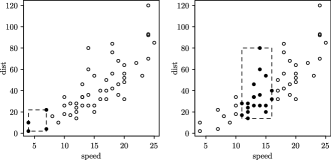
Figure 2: Brush a scatterplot using the MVC design: brush the first four points (left), then brush all points from the 10th to 28th. The dashed rectangle denotes the “brush,” which is normally created by dragging the cursor over the points. The cars data is a data set in base R. It has been ordered first by speed and then dist in the increasing order, so the bottom-left point is the first observation in the data.

Now our only task is to assign indices of the brushed points to reactiveBrush, since the plot will be updated automatically. A real interactive graphics system is more complicated than the above toy example, but it shows the foundation of the pipeline. The two kinds of interactive objects in cranvas are explained in the next two sections, respectively.

3.1 Mutaframes

A mutaframe is an extension to the R data frame. They are mutable, which means that changes to its elements can be made anywhere regardless of the current environment. By comparison, a data frame can only be modified in the environment in which it was created, unless we use the nonlocal assignment operator <<-. The difference is highlighted in the example below.

As we can see, mf can be modified inside f(), but df cannot, therefore, we can share the same mutaframe across multiple plots. Another important feature of mutaframes is that we can attach listeners to them. A listener is essentially an R function which is called upon changes in the mutaframe. For interactive graphics, views are updated with listeners. Below we create a mutaframe and attach a listener to it to redraw the scatterplot.

Now whenever we update mf, the scatterplot will be updated accordingly. For example, we make a square-root transformation of the dist variable (see Figure 3 for the original plot and the transformed version).

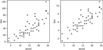
Figure 3: The original scatterplot (left) is automatically updated (right) when the dist variable is square-root transformed (right). We can also modify the speed variable or change the values of some rows in the data to update the plot.

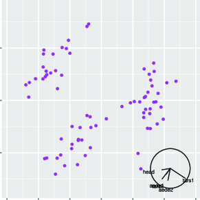
Figure 4: A grand tour through the flea data. The points are separated into three clusters. Watch the video online at http://cranvas.org/examples/qtour.html.

A more complex but direct application of mutaframes is the example shown in the movie displayed in Figure 4: here, we see a two-dimensional grand tour (Asimov, 1985) through the flea data set provided in the tourr package (Wickham et al., 2011). A two-dimensional tour consists of a series of projections into two-dimensional space. By choosing close consecutive projections, a sense of continuity is preserved for the observer. This continuity allows us to identify clusters as groups of points that share a common fate (e.g., Wolfe, Kluender and Levi (2012)). Internally, the movie is created by repeated changes to the $X$ and $Y$ values displayed in a scatterplot, which are propagated to the view.

Interactivity of a mutaframe can be propagated to its subsets, which allows multiple applications based on one mutaframe and its offsprings. For instance, we can select a subset of points in a scatterplot, obtain their indices and use the indices to subset the original mutaframe to draw a new plot. The new plot is then automatically connected with the original plot: when we interact with the new plot, the selection will be passed to the mutaframe and propagated to the original plot. This is similar to an example described in early work by Hurley and Oldford (1988).

3.2 Reference Classes

R reference classes were introduced in R version 2.12. This made it possible to create objects with fields that can be accessed by reference. A consequence of this feature is that such objects can be used for storing metadata in the graphics system, and the data can be modified outside of plotting functions. For instance, we can store the axis limits in an object meta as meta$limits. In the terminology of reference classes, limits is called a field of meta. After the plot has been drawn, we are still able to modify its limits and the new limits will be available to the internal drawing subroutines of the plotting function. This is inconvenient, if not impossible, under the usual copy-on-modify semantics in R. The brushing example in Figure 2 is rewritten using reference classes.

We created a reference class object obj from the constructor objBrush, and this object has a field called .brushed which is a logical vector to store the brush status. The other field brushed is a function that acts as the controller: we can assign new values to it, and the view will be updated accordingly. We can also query the current brush status to, for example, explore the brushed subset of the data separately. The object obj can be modified anywhere in the system as desired, which is often not the case for normal R objects. We will show how reference classes work for interactions in single display applications later.

What is more important is the extension by the objectSignals package (Lawrence and Yin, 2011) based on reference classes. The objects created from this package are called “signal objects,” which are basically special reference classes objects with listeners attached on them. This is similar to mutaframes described before, but we can create objects of arbitrary structures. The difference between mutaframes and signal objects is similar to the difference between data frames and lists in R.

3.3 Reactive Programming Behind Cranvas

Mutaframes and reference classes objects are extensively used in cranvas, although this may not be immediately obvious to the users. Below we show some quick examples based on the Ames housing data (Ames, IA, 2008–2012). Before we draw any plots in cranvas, we have to create a mutaframe using the function qdata().

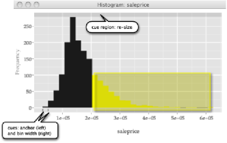
Figure 5: Histogram of sales prices. Sales of $200k and more are selected and highlighted in yellow. Markers show visual cues. See http://cranvas.org/examples/qhist.html for a video of the interactions.

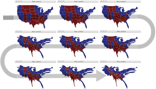
Figure 6: Morph from a choropleth chart of the US (top left) to a population-based cartogram (bottom right). The color represents electoral votes of states toward the Democratic (blue) or Republican party (red) in the 2012 Presidential election. The arrow indicates the direction of the morph.

The function qhist() draws a histogram of the sale price, qbar() draws a bar chart of the number of bathrooms, and qscatter() draws a scatterplot of the sale price against the living area. All plotting functions have to take a data argument, which is a mutaframe. Inside each function, listeners will be built on the data so changes in the plot can be propagated back to the data object and further passed to other plots.

The returned value of a plotting function contains the signal object, which can be retrieved from the attributes of the returned value. The user can manipulate the signal object and the plot can respond to the changes because a number of listeners have been attached to it internally when we call the plotting function.

Figures 5 and 11 show the histogram and the bar chart from the above R code. We will present details about the reactive objects in the next section.

4 An Anatomy of Interactions

In this section we show how some common interactions, including brushing, zooming and querying, etc, were implemented in cranvas. The data infrastructure is based on mutaframes and reference classes/signal objects, as introduced in the previous section. The actual drawing is based on the packages qtbase (Lawrence and Sarkar, 2013a) and qtpaint (Lawrence and Sarkar, 2013b), which provide an interface from R to Qt (Verzani and Lawrence, 2012).

4.1 Input Actions

Interaction with a system involves user actions as the input to the system, then the system resolves the input information and responds to the user. Interaction happens on multiple levels of user actions. The most common forms of interaction with a display are listed below in decreasing order of immediacy with which this interaction between the user and the display happens:

Direct manipulation of graphical objects (Shneiderman, 1983; Swayne and Klinke (1999); Wills (1999)) is at the heart of interactive graphics. Direct manipulation is what we use only for the highest level of interaction, such as selection or brushing of elements. With a set of different modes (querying, scaling mode as, for example, implemented in XGobi/GGobi), a set of different or additional interactions can be incorporated at the highest level. Another approach is to make use of visual cues, which suggest available interactions to the user, for example, changing the cursor upon entering the cue area. Visual cues are usually associated with changes to the resolution of a representation or scales of a display. Figure 5 shows an example of a plot with visual cues.

Input devices such as a mouse or touch pad allow interaction beyond click selection. Most toolkits support wheel events (either through the presence of a mouse wheel, a mouse move with an additional modifier key or a touch gesture), and a wheel event often corresponds to the zooming of a plot.

Keystrokes can be used as shortcuts and for quick access to functions. Figure 6 shows an example of a key stroke interaction (arrow keys Left and Right) to move between a choropleth map of the United States and a population-based cartogram.

Functional access through the command-line: Accessor functions allow us to get information about the state of objects (e.g., get the indices of selected elements). Mutator functions enable the user to set a particular state for objects in a display (e.g., set highlighting color to red, set points to size 5). We call this level of interaction “indirect manipulation” of graphics.

On the developer’s side, the main idea behind resolving an interaction between the user and the display is to actually resolve the interaction at the level of the data, but make it appear as if the user had directly interacted with the graphical object. This is essentially what happens in cranvas when we interact with plots.

All levels of interaction above are supported in cranvas, and both direct and indirect manipulation are available. At its core, all kinds of manipulation end up as changes to the underlying data objects, which is described in the next section.

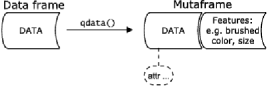
Figure 7: The conversion from a data frame to a mutaframe, which can be imagined as an augmented and mutable data frame. Additional columns for the brush status and aesthetics of graphical elements are appended to the original data frame.

4.2 Reactive Data Objects

Figure 7 illustrates the first step in cranvas, to create a mutaframe. The function qdata() in cranvas returns a mutaframe with additional columns. Below is a simple example.

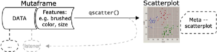
Figure 8: Create a scatterplot and attach a metaobject to it.

The data frame cars was augmented by columns such as .brushed and .color. The .brushed column indicates the brush status of graphical elements (TRUE means an element is brushed), and .color stores the colors of elements. It is up to a specific plot how to interpret these additional columns. For example, in scatterplots, because each row in the data corresponds to a point in the plot, points can be colored by .color and highlighted by the logical in .brushed. For a bar chart, displaying frequencies of a categorical variable, .brushed may result in a partially or fully highlighted bar when only a subset in a category is brushed.

Each single display application in cranvas creates a plot and attaches listeners on the mutaframe at the same time. Figure 8 shows how a scatterplot is created from a mutaframe: before the qscatter() function displays the plot, it binds the augmented columns in the mutaframe with the plot layers using listener functions, so that when these columns are updated, the plot can be updated. The Qt graphics framework allows us to build a plot using layers, which makes it possible to update one component of a plot without having to update all others. This gives us a lot of performance gain, especially when we interact with plots of large numbers of elements. In cranvas, the .color column should update the main layer of points and the .brushed column controls the brush layer. See http://cranvas.org/2013/10/qt-performance/ for an example of brushing a scatterplot of three million points, which takes less than 0.01 second to render, and is highly responsive to the brush. The main plot layer of three million points is not redrawn when the brush moves over the plot, only the brush layer.

The other type of reactive data objects in cranvas are the metadata. Such objects often contain plot-specific information, such as the names of variables in the plot and the axis limits, etc. When a plot is created, a copy of metadata is generated and associated with it. Zooming (http://cranvas.org/examples/qscatter.html) is an example. Behind the scenes the axis limits are modified in the metadata based on the mouse wheel event.

Since the data structure of metaobjects is flexible, its application can be broad. The cranvas package allows adding or customizing meta information to any displays. For example, the user can specify a function in the metaobject to generate text labels when querying a plot. In the following text, we use meta to denote a metadata object.

4.3 Interactions

This section describes the interactions supported in cranvas and how they are related to the reactive data objects.

4.3.1 Brushing and selection

Brushing and selection are interactions that highlight a subset of graphical elements in a plot. It is usually achieved by dragging a rectangle (or other closed shape) over a plot and the elements inside the rectangle are selected. The rectangle, when in the brushing mode, is persistent on the screen. For the selection mode, the rectangle is transient, meaning that it disappears when the mouse is released.

We use the qscatter() function to illustrate the basic idea. We show a sketch using the pseudo code below.

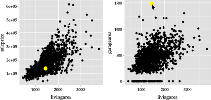
Figure 9: One-to-one linking: we highlight the house with the largest garage in the right plot and this house is also highlighted in the left plot. Apparently it is not of the highest price.

There are two layers layer_main and layer_brush in the plot. The brush layer is used to redraw the brushed points only, so that the main layer can stay untouched when points are highlighted. The key for brushing/selection is the listener added to the mutaframe data by add_listener(): when the column x, y or .brushed is modified, the brush layer is updated (changes in other columns will not affect the plot). Adding the listener is denoted by the dashed arrow in Figure 8.

When the plot is brushed, the points under the brush are identified by the mouse events in Qt and the .brushed variable in the mutaframe is modified. Because of the listener associated with .brushed, the brush layer will be redrawn. Therefore, the selection is actually handled with one step of backtracking: once the user draws a selection rectangle, we update .brushed immediately, which triggers the update of the brush layer. Because this occurs in a fast pace, the user may have an illusion that the cursor directly selected the points. See Figure 9 for an example of brushing scatterplots of the Ames housing data (R code is provided in the next section). The selection mode was used in these plots, so we do not see the brush rectangle. Brushing mode was used in Figure 5 and the yellow rectangle illustrates brush position.

In the case of a histogram, bins are the graphical objects intersecting with a selection rectangle. The backtracking corresponds to identifying all records in the mutaframe falling within the limits of the selected bin. The binary variable .brushed is changed when the brush moves over the bins, and the change is propagated to all dependencies, which results in an update to all dependent views. One of the dependent views is the histogram itself, which shows highlighting in the form of superimposing a histogram of the highlighted records on top of the original histogram. What the user perceives as “selecting” bins is actually a reaction to a change in the internal brushing variable.

4.3.2 Linking

Linking forms the core of communication between multiple views. By default, all views that involve variables from the same mutaframe are linked. Linking within the same data set is implicitly one-to-one linking.

Using the mutaframe qames from Section 3.3, two scatterplots are created (Figure 9) and illustrate one-to-one linking.

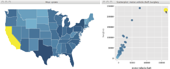
Figure 10: Linked map (left) and scatterplot (right). Color shading shows (log) state population with darker shades indicating higher values. The scatterplot on the right displays the number of burglaries in 2009 versus the number of motor vehicle thefts by state. There is a strong correlation between the variables, which is mainly induced by a strong underlying correlation with population. Compared to other states, California displays a high number of motor vehicle thefts compared to the number of burglaries.

The selected property has extraordinarily large garage area, for the living area, and has a below average sale price.

Recall from the previous section that when a scatterplot is created, a listener to update the brush layer is attached to the mutaframe. It does not matter where the mutaframe is modified, all the brush layers will be updated if the .brushed variable in the mutaframe is modified. When we interact with either of the plots, the other plot will respond to the changes because both plots depend on the .brushed variable in the same mutaframe.

It is feasible to extend this concept to link different sources or aggregation levels of the data. Take the following two types of linking, for example:

Categorical linking means when we brush one or more observations in one category, all observations in this category are brushed; this is achieved in the listener by setting all elements of .brushed in this category to TRUE;

kNN linking ($k$ nearest neighbor) means when we brush an observation, its $k$ nearest neighbors under a certain distance metric are brushed as well; again, this is nothing but setting the relevant elements in .brushed to TRUE.

They can be applied to a single data source (called “self-linking”) or multiple data sources. In the latter case, the listener in one data object needs to update other data objects. In Figure 10, the map and the scatterplot use two different sources, and they are linked via categorical linking through the state names. Each state in the map is described by multiple points defining the state boundary, but each state has only one observation in the scatterplot. If we brush California in the scatterplot, the whole polygon of California (containing multiple locations) is highlighted. On the other hand, if we brush a part of a state in the map, that means the whole state should be highlighted, which is an example of self-linking.

Linking can also be done on the same data with different aggregation levels, such as the raw data and binned data. The histogram in Figure 5 shows sales prices of all houses sold in the Ames housing data. The yellow rectangle corresponds to an area-based selection of all houses with sales of $200k or more, which triggers a highlighting of corresponding houses in all displays of the Ames housing data. This includes the histogram itself, where all bins intersecting with the selection rectangle are filled with highlighting color, and all bar charts of the number of bedrooms as shown in Figure 11.

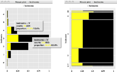
Figure 11: Bar chart (left) and spine plot (right) of the number of bedrooms in housing sales. Highlighted are sales of $200k and higher. Querying gives details on each bin (houses with a particular number of bedrooms) and the selected houses with this bin.

4.3.3 Zooming and panning

Zooming and panning change or shift the scale of the view, so we can see the data at different resolutions. This can be resolved directly without the need of interaction with the original data. In cranvas, the core of zooming and panning consists of simple changes to the metadata meta$limits. This is illustrated with the following pseudo code.

Scatter is a constructor created from reference classes, containing a field named limits in meta. The key here is to set up the event meta$limitsChanged: this event is triggered when meta$limits is modified and the axis limits of the main plot layer are replaced by the new value of meta$limits. The setLimits() method is from Qt, which is used to set new limits on a layer, and Qt will update the view when the limits are changed.

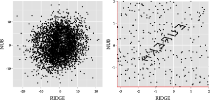
Figure 12: Zooming into the pollen data. The original scatterplot (left) does not show anything interesting, but as we zoom into the plot, we see a hidden word “EUREKA.”

In cranvas, meta$limits is modified by the mouse wheel event for zooming and by the mouse drag event for panning. Figure 12 shows two screenshots of the original scatterplot and the zoomed version, respectively.

A benefit of controlling the limits in this manner is that it is a local property of the plot, enabling the user to examine different resolutions in two different displays.

4.3.4 Querying/identifying

Querying/identifying is another interaction that can usually be resolved without information from the original data. Querying of graphical objects involves, in a first step, the display of the corresponding values of the metadata. For the bar charts in Figure 11, querying of the bins displays information, about the bin’s level and the number of records it encompasses, as well as the proportion of the whole data that this bin contains.

4.3.5 Visual cues

Visual cues aid the user to learn about available interactions. Figure 5 shows several examples of visual cues in a histogram. Both the anchor point and bin width are graphical representations of plotting parameters for the histogram. The anchor of a histogram is the lower limit of the leftmost bin. The bin width defines the interval at which breaks are made. Interacting with either anchor or bin width cues produces horizontal shifts, which reset the actual values parametrizing the histogram. Changes to the anchor allow for testing of instabilities in the display due to discreteness in the data. Bin-width changes show the data at different levels of smoothness and therefore allow for a visualization of “big” picture marginal distributions at large bin widths and the investigation of small pattern features, such as multiple modes and gaps in the data, at small bin widths. Examples for both of these interactions are available as movies in the supplementary material of this paper.

The visual cues in this case also correspond to meta elements. Specifically, the bin limits are stored in meta$breaks and the histogram layer is connected to the meta$breaksChanged event. The anchor modifies meta$breaks when we drag it.

5 Conclusions

The concept of MVC is made implicit in reactive programming. Reactive data objects are used to manage the multiple views and interactions in the cranvas package.

The cranvas package is built on graphics layers in Qt (frontend) and reactive data objects in R (backend). The plotting pipeline is expressed and attached to mutaframes as well as metadata objects. Using the reactive programming model, the user does not need to pay attention to the whole pipeline, which makes it easy to extend this system. For example, implementing the tour is simply redrawing a scatterplot of the projected variables that keep changing because the mutaframe will update the view automatically upon changes.

The future work of cranvas involves including more plot types such as hexbin plots and scatterplot matrices, allowing users to define how the system reacts to changes and adding a GUI. The qtbase package has made it easy to build Qt GUI’s in R. The GUI widgets can be connected to the plots via reactive data objects. They do not need to know the internal structure of plots. This kind of modularity will make the system easier to maintain and extend than past graphics software.

Supplementary Materials

The cranvas package is available on GitHub at https://github.com/ggobi/cranvas. We have movies showing some interactions that are available on the website http://cranvas.org.

References

- Asimov (1985) {barticle}[mr] \bauthor\bsnmAsimov, \bfnmDaniel\binitsD. (\byear1985). \btitleThe grand tour: A tool for viewing multidimensional data. \bjournalSIAM J. Sci. Statist. Comput. \bvolume6 \bpages128–143. \biddoi=10.1137/0906011, issn=0196-5204, mr=0773286 \bptokimsref\endbibitem
- Bostock, Ogievetsky and Heer (2011) {barticle}[auto:STB—2014/02/12—14:17:21] \bauthor\bsnmBostock, \bfnmMichael\binitsM., \bauthor\bsnmOgievetsky, \bfnmVadim\binitsV. and \bauthor\bsnmHeer, \bfnmJeffrey\binitsJ. (\byear2011). \btitleD3 data-driven documents. \bjournalIEEE Transactions on Visualization and Computer Graphics \bvolume17 \bpages2301–2309. \bptokimsref\endbibitem
- Buja et al. (1988) {bincollection}[auto:STB—2014/02/12—14:17:21] \bauthor\bsnmBuja, \bfnmAndreas\binitsA., \bauthor\bsnmAsimov, \bfnmDaniel\binitsD., \bauthor\bsnmHurley, \bfnmCatherine\binitsC. and \bauthor\bsnmMcDonald, \bfnmJohn A.\binitsJ. A. (\byear1988). \btitleElements of a viewing pipeline for data analysis. In \bbooktitleDynamic Graphics for Statistics \bpages277–308. \bpublisherWadsworth & Brooks/Cole, \blocationBelmont, CA. \bptokimsref\endbibitem
- Chambers (2013) {bmisc}[auto:STB—2014/02/12—14:17:21] \bauthor\bsnmChambers, \bfnmJohn\binitsJ. (\byear2013). \bhowpublishedObjects with fields treated by reference (OOP-style). See help(ReferenceClasses) in R. \bptokimsref\endbibitem
- Cook and Swayne (2007) {bbook}[auto:STB—2014/02/12—14:17:21] \bauthor\bsnmCook, \bfnmDianne\binitsD. and \bauthor\bsnmSwayne, \bfnmDeborah F.\binitsD. F. (\byear2007). \btitleInteractive and Dynamic Graphics for Data Analysis with R and GGobi. \bpublisherSpringer, \blocationBerlin. \bptokimsref\endbibitem
- Dykes (1998) {barticle}[auto:STB—2014/02/12—14:17:21] \bauthor\bsnmDykes, \bfnmJason\binitsJ. (\byear1998). \btitleCartographic visualization: Exploratory spatial data analysis with local indicators of spatial association using Tcl/Tk and cdv. \bjournalJournal of the Royal Statistical Society: Series D (The Statistician) \bvolume47 \bpages485–497. \bptokimsref\endbibitem
- Fisherkeller, Friedman and Tukey (1988) {bincollection}[auto:STB—2014/02/12—14:17:21] \bauthor\bsnmFisherkeller, \bfnmMary A.\binitsM. A., \bauthor\bsnmFriedman, \bfnmJerome H.\binitsJ. H. and \bauthor\bsnmTukey, \bfnmJohn W.\binitsJ. W. (\byear1988). \btitlePRIM-9: An interactive multidimensional data display and analysis system. In \bbooktitleDynamic Graphics for Statistics \bpages91–109. \bpublisherWadsworth & Brooks/Cole, \blocationBelmont, CA. \bptokimsref\endbibitem
- Hurley and Oldford (1988) {bmisc}[auto:STB—2014/02/12—14:17:21] \bauthor\bsnmHurley, \bfnmC.\binitsC. and \bauthor\bsnmOldford, \bfnmR. W.\binitsR. W. (\byear1988). \bhowpublishedHigher hierarchical views of statistical objects. Available from the video library of the ASA sections on Statistical Graphics: http://stat-graphics.org/movies/. \bptokimsref\endbibitem
- Krasner and Pope (1988) {barticle}[auto:STB—2014/02/12—14:17:21] \bauthor\bsnmKrasner, \bfnmGlenn E.\binitsG. E. and \bauthor\bsnmPope, \bfnmStephen T.\binitsS. T. (\byear1988). \btitleA cookbook for using the model-view controller user interface paradigm in Smalltalk-80. \bjournalJournal of Object-Oriented Programming \bvolume1 \bpages26–49. \bptokimsref\endbibitem
- Lawrence and Sarkar (2013a) {bmisc}[auto:STB—2014/02/12—14:17:21] \bauthor\bsnmLawrence, \bfnmMichael\binitsM. and \bauthor\bsnmSarkar, \bfnmDeepayan\binitsD. (\byear2013a). \bhowpublishedqtbase: Interface between R and Qt. R package version 1.0.6. \bptokimsref\endbibitem
- Lawrence and Sarkar (2013b) {bmisc}[auto:STB—2014/02/12—14:17:21] \bauthor\bsnmLawrence, \bfnmMichael\binitsM. and \bauthor\bsnmSarkar, \bfnmDeepayan\binitsD. (\byear2013b). \bhowpublishedqtpaint: Qt-based painting infrastructure. R package version 0.9.0. \bptokimsref\endbibitem
- Lawrence and Temple Lang (2010) {barticle}[auto:STB—2014/02/12—14:17:21] \bauthor\bsnmLawrence, \bfnmMichael\binitsM. and \bauthor\bsnmTemple Lang, \bfnmDuncan\binitsD. (\byear2010). \btitleRGtk2: A graphical user interface toolkit for R. \bjournalJournal of Statistical Software \bvolume37 \bpages1–52. \bptokimsref\endbibitem
- Lawrence and Wickham (2012) {bmisc}[auto:STB—2014/02/12—14:17:21] \bauthor\bsnmLawrence, \bfnmMichael\binitsM. and \bauthor\bsnmWickham, \bfnmHadley\binitsH. (\byear2012). \bhowpublishedplumbr: Mutable and dynamic data models. R package version 0.6.6. \bptokimsref\endbibitem
- Lawrence and Yin (2011) {bmisc}[auto:STB—2014/02/12—14:17:21] \bauthor\bsnmLawrence, \bfnmMichael\binitsM. and \bauthor\bsnmYin, \bfnmTengfei\binitsT. (\byear2011). \bhowpublishedMutable signal objects. R package version 0.10.2. \bptokimsref\endbibitem
- Leff and Rayfield (2001) {bincollection}[auto:STB—2014/02/12—14:17:21] \bauthor\bsnmLeff, \bfnmAvraham\binitsA. and \bauthor\bsnmRayfield, \bfnmJames T.\binitsJ. T. (\byear2001). \btitleWeb-application development using the model/view/controller design pattern. In \bbooktitleIEEE Enterprise Distributed Object Computing Conference \bpages118–127. \bpublisherIEEE. \bptokimsref\endbibitem
- McDonald, Stuetzle and Buja (1990) {bincollection}[auto:STB—2014/02/12—14:17:21] \bauthor\bsnmMcDonald, \bfnmJohn Alan\binitsJ. A., \bauthor\bsnmStuetzle, \bfnmWerner\binitsW. and \bauthor\bsnmBuja, \bfnmAndreas\binitsA. (\byear1990). \btitlePainting multiple views of complex objects. In \bbooktitleACM SIGPLAN Notices 25 \bpages245–257. \bpublisherACM, \blocationNew York. \bptokimsref\endbibitem
- Qt Project (2013) {bmisc}[auto:STB—2014/02/12—14:17:21] \bauthor\borganizationQt Project (\byear2013). \bhowpublishedA cross-platform application and UI framework. Available at http://qt-project.org/. \bptokimsref\endbibitem
- R Core Team (2013) {bmisc}[auto:STB—2014/02/12—14:17:21] \bauthor\borganizationR Core Team (\byear2013). \bhowpublishedR: A Language and Environment for Statistical Computing. R Core Team, Vienna, Austria. \bptokimsref\endbibitem
- Rosling and Johansson (2009) {barticle}[auto:STB—2014/02/12—14:17:21] \bauthor\bsnmRosling, \bfnmH.\binitsH. and \bauthor\bsnmJohansson, \bfnmC.\binitsC. (\byear2009). \btitleGapminder: Liberating the X-axis from the burden of time. \bjournalStatistical Computing and Statistical Graphics Newsletter \bvolume20 \bpages4–7. \bptokimsref\endbibitem
- RStudio, Inc. (2013) {bmisc}[auto:STB—2014/02/12—14:17:21] \bauthor\borganizationRStudio, Inc. (\byear2013). \bhowpublishedEasy web applications in R. Available at http://www.rstudio.com/shiny/. \bptokimsref\endbibitem
- SAS Institute (2009) {bmisc}[auto:STB—2014/02/12—14:17:21] \bauthor\borganizationSAS Institute (\byear2009). \bhowpublishedJMP 8 Statistics and Graphics Guide. SAS Publishing, Cary, NC. \bptokimsref\endbibitem
- Shneiderman (1983) {barticle}[auto:STB—2014/02/12—14:17:21] \bauthor\bsnmShneiderman, \bfnmB.\binitsB. (\byear1983). \btitleDirect manipulation: A step beyond programming languages. \bjournalComputer \bvolume16 \bpages57–69. \bptokimsref\endbibitem
- Stuetzle (1987) {barticle}[auto:STB—2014/02/12—14:17:21] \bauthor\bsnmStuetzle, \bfnmWerner\binitsW. (\byear1987). \btitlePlot Windows. \bjournalJ. Amer. Statist. Assoc. \bvolume82 \bpages466–475. \bptokimsref\endbibitem
- Swayne and Klinke (1999) {barticle}[auto:STB—2014/02/12—14:17:21] \bauthor\bsnmSwayne, \bfnmDeborah F.\binitsD. F. and \bauthor\bsnmKlinke, \bfnmSigbert\binitsS. (\byear1999). \btitleIntroduction to the Special issue on interactive graphical data analysis: What is interaction? \bjournalComput. Statist. \bvolume14 \bpages1–6. \bptokimsref\endbibitem
- Swayne et al. (2003) {barticle}[mr] \bauthor\bsnmSwayne, \bfnmDeborah F.\binitsD. F., \bauthor\bsnmTemple Lang, \bfnmDuncan\binitsD., \bauthor\bsnmBuja, \bfnmAndreas\binitsA. and \bauthor\bsnmCook, \bfnmDianne\binitsD. (\byear2003). \btitleGGobi: Evolving from XGobi into an extensible framework for interactive data visualization. \bjournalComput. Statist. Data Anal. \bvolume43 \bpages423–444. \biddoi=10.1016/S0167-9473(02)00286-4, issn=0167-9473, mr=2005447 \bptokimsref\endbibitem
- Theus (2002) {barticle}[auto:STB—2014/02/12—14:17:21] \bauthor\bsnmTheus, \bfnmMartin\binitsM. (\byear2002). \btitleInteractive data visualization using Mondrian. \bjournalJournal of Statistical Software \bvolume7 \bpages1–9. \bptokimsref\endbibitem
- Tierney (1990) {bbook}[auto:STB—2014/02/12—14:17:21] \bauthor\bsnmTierney, \bfnmLuke\binitsL. (\byear1990). \btitleLISP-STAT: An Object-Oriented Environment for Statistical Computing and Dynamic Graphics. \bpublisherWiley, \blocationNew York. \bptokimsref\endbibitem
- Tierney (2005) {barticle}[auto:STB—2014/02/12—14:17:21] \bauthor\bsnmTierney, \bfnmLuke\binitsL. (\byear2005). \btitleSome notes on the past and future of LISP-STAT. \bjournalJournal of Statistical Software \bvolume13 \bpages1–15. \bptokimsref\endbibitem
- Unwin et al. (1996) {barticle}[auto:STB—2014/02/12—14:17:21] \bauthor\bsnmUnwin, \bfnmA. R.\binitsA. R., \bauthor\bsnmHawkins, \bfnmG.\binitsG., \bauthor\bsnmHofmann, \bfnmH.\binitsH. and \bauthor\bsnmSiegl, \bfnmB.\binitsB. (\byear1996). \btitleInteractive graphics for data sets with missing values—MANET. \bjournalJ. Comput. Graph. Statist. \bvolume5 \bpages113–122. \bptokimsref\endbibitem
- Urbanek and Wichtrey (2013) {bmisc}[auto:STB—2014/02/12—14:17:21] \bauthor\bsnmUrbanek, \bfnmSimon\binitsS. and \bauthor\bsnmWichtrey, \bfnmTobias\binitsT. (\byear2013). \bhowpublishediplots: iPlots—Interactive graphics for R. R package version 1.1-5. \bptokimsref\endbibitem
- Velleman and Velleman (1988) {bmisc}[auto:STB—2014/02/12—14:17:21] \bauthor\bsnmVelleman, \bfnmP. F.\binitsP. F. and \bauthor\bsnmVelleman, \bfnmA. Y.\binitsA. Y. (\byear1988). \bhowpublishedData Desk Handbook. Odesta Corporation, Northbrook, IL. \bptokimsref\endbibitem
- Verzani and Lawrence (2012) {bbook}[auto:STB—2014/02/12—14:17:21] \bauthor\bsnmVerzani, \bfnmJohn\binitsJ. and \bauthor\bsnmLawrence, \bfnmMichael F.\binitsM. F. (\byear2012). \btitleProgramming Graphical User Interfaces in R. \bpublisherChapman & Hall/CRC, \blocationLondon. \bptokimsref\endbibitem
- Viegas et al. (2007) {barticle}[auto:STB—2014/02/12—14:17:21] \bauthor\bsnmViegas, \bfnmFernanda B.\binitsF. B., \bauthor\bsnmWattenberg, \bfnmMartin\binitsM., \bauthor\bsnmVan Ham, \bfnmFrank\binitsF., \bauthor\bsnmKriss, \bfnmJesse\binitsJ. and \bauthor\bsnmMcKeon, \bfnmMatt\binitsM. (\byear2007). \btitleManyeyes: A site for visualization at internet scale. \bjournalIEEE Transactions on Visualization and Computer Graphics \bvolume13 \bpages1121–1128. \bptokimsref\endbibitem
- Whalen (2005) {bmisc}[auto:STB—2014/02/12—14:17:21] \bauthor\bsnmWhalen, \bfnmElizabeth\binitsE. (\byear2005). \bhowpublishedCreating linked, interactive views to explore multivariate data. Ph.D. thesis, Harvard Univ. \bptokimsref\endbibitem
- Wickham et al. (2008) {barticle}[auto:STB—2014/02/12—14:17:21] \bauthor\bsnmWickham, \bfnmHadley\binitsH., \bauthor\bsnmLawrence, \bfnmMichael\binitsM., \bauthor\bsnmTemple Lang, \bfnmDuncan\binitsD. and \bauthor\bsnmSwayne, \bfnmDeborah F.\binitsD. F. (\byear2008). \btitleAn introduction to rggobi. \bjournalR News \bvolume8 \bpages3–7. \bptokimsref\endbibitem
- Wickham et al. (2009) {barticle}[mr] \bauthor\bsnmWickham, \bfnmHadley\binitsH., \bauthor\bsnmLawrence, \bfnmMichael\binitsM., \bauthor\bsnmCook, \bfnmDianne\binitsD., \bauthor\bsnmBuja, \bfnmAndreas\binitsA., \bauthor\bsnmHofmann, \bfnmHeike\binitsH. and \bauthor\bsnmSwayne, \bfnmDeborah F.\binitsD. F. (\byear2009). \btitleThe plumbing of interactive graphics. \bjournalComput. Statist. \bvolume24 \bpages207–215. \biddoi=10.1007/s00180-008-0116-x, issn=0943-4062, mr=2506079 \bptokimsref\endbibitem
- Wickham et al. (2011) {bmisc}[auto:STB—2014/02/12—14:17:21] \bauthor\bsnmWickham, \bfnmHadley\binitsH., \bauthor\bsnmCook, \bfnmDianne\binitsD., \bauthor\bsnmHofmann, \bfnmHeike\binitsH. and \bauthor\bsnmBuja, \bfnmAndreas\binitsA. (\byear2011). \bhowpublishedtourr: An R package for exploring multivariate data with projections. Journal of Statistical Software 40 1–18. \bptokimsref\endbibitem
- Wills (1999) {bincollection}[auto:STB—2014/02/12—14:17:21] \bauthor\bsnmWills, \bfnmGraham J.\binitsG. J. (\byear1999). \btitleInteractive statistical graphics. In \bbooktitleHandbook of Data Mining and Knowledge Discovery. \bpublisherOxford Univ. Press, \blocationLondon. \bptokimsref\endbibitem
- Wolfe, Kluender and Levi (2012) {bbook}[auto:STB—2014/02/12—14:17:21] \bauthor\bsnmWolfe, \bfnmJ. M.\binitsJ. M., \bauthor\bsnmKluender, \bfnmK. R.\binitsK. R. and \bauthor\bsnmLevi, \bfnmD. M.\binitsD. M. (\byear2012). \btitleSensation and Perception, \bedition3rd ed. \bpublisherSinauer, \blocationSunderland. \bptokimsref\endbibitem
- Xie et al. (2013) {bmisc}[auto:STB—2014/02/12—14:17:21] \bauthor\bsnmXie, \bfnmYihui\binitsY., \bauthor\bsnmHofmann, \bfnmHeike\binitsH., \bauthor\bsnmCook, \bfnmDi\binitsD., \bauthor\bsnmCheng, \bfnmXiaoyue\binitsX., \bauthor\bsnmSchloerke, \bfnmBarret\binitsB., \bauthor\bsnmVendettuoli, \bfnmMarie\binitsM., \bauthor\bsnmYin, \bfnmTengfei\binitsT., \bauthor\bsnmWickham, \bfnmHadley\binitsH. and \bauthor\bsnmLawrence, \bfnmMichael\binitsM. (\byear2013). \bhowpublishedcranvas: Interactive statistical graphics based on Qt. R package version 0.8.3. Available at http://cranvas.org. \bptokimsref\endbibitem