$\mathcal{P}\mathcal{T}$-Symmetric dimer in a generalized model of coupled nonlinear oscillators

Abstract

In the present work, we explore the case of a general $\mathcal{PT}$-symmetric dimer in the context of two both linearly and nonlinearly coupled cubic oscillators. To obtain an analytical handle on the system, we first explore the rotating wave approximation converting it into a discrete nonlinear Schrödinger type dimer. In the latter context, the stationary solutions and their stability are identified numerically but also wherever possible analytically. Solutions stemming from both symmetric and anti-symmetric special limits are identified. A number of special cases are explored regarding the ratio of coefficients of nonlinearity between oscillators over the intrinsic one of each oscillator. Finally, the considerations are extended to the original oscillator model, where periodic orbits and their stability are obtained. When the solutions are found to be unstable their dynamics is monitored by means of direct numerical simulations.

I Introduction

The notion of parity-time ($\mathcal{P}\mathcal{T}$) symmetry has recently been receiving increasing attention over a wide variety of settings; see e.g. Bender_review ; special-issues ; review . The original proposal involved a non-Hermitian variant of quantum mechanics which might still produce real eigenvalues (and hence be associated with measurable quantities). However, it was instead the analogy of this model with the paraxial approximation in optics which led to the proposal that such mathematical constructs can be realized in optical settings Muga ; PT_periodic , and which eventually led to their experimental realization experiment . This series of developments, in turn, prompted researchers towards a more detailed understanding of the stationary states of such $\mathcal{P}\mathcal{T}$-systems (and how they differ from their Hamiltonian analogues), an effort to appreciate their stability properties and finally an attempt to quantify their nonlinear dynamics. This effort emerged both at the level of few-site configurations Dmitriev ; Li ; Guenter ; Ramezani ; suchkov ; Sukhorukov ; ZK ; MKK ; CW (which were chiefly experimentally accessible), as well as at that of infinite-size lattices Pelin1 ; Sukh ; zheng .

Although the quantum-mechanical and paraxial-optical focal points of this activity have provided an emphasis on the study of Schrödinger type settings, a number of recent studies, especially on the experimental side, have led to an increased interest in oscillator systems (which one can think of as oligomers -few site settings- of the Klein-Gordon type). More specifically, a mechanical system realizing $\mathcal{P}\mathcal{T}$-symmetry has been proposed in pt_mech , while a major thrust of research has focused on the context of electronic circuits; see e.g. the original realization of tsampikos_recent and the more recent review of this activity in tsampikos_review . As an aside, we note that additional intriguing realizations of $\mathcal{P}\mathcal{T}$-symmetry have also emerged e.g. in the realm of whispering-gallery microcavities pt_whisper . Mostly, the efforts on this oscillator realm have been limited to the study of linear systems, yet recently a number of nonlinear variants have been explored both theoretically/numerically and even experimentally. As notable such examples, we mention the split-ring resonator chain in the context of magnetic metamaterials proposed in the work of tsironis , as well as the experimental realization of a $\mathcal{P}\mathcal{T}$-symmetric dimer of Van-der-Pol oscillators that arose in the work of bend_kott .

On the theoretical side, some of these studies raised a number of intriguing theoretical questions. For instance, the theoretical modeling of the linear $\mathcal{P}\mathcal{T}$-symmetric analogue of the system pt_whisper led to the realization that such linear oscillator pairs may be Hamiltonian although one of them has gain and the other has loss bend_gian . This, in turn, led the authors of bar_gian to appreciate that this feature (the Hamiltonian nature of a $\mathcal{P}\mathcal{T}$-symmetric oscillator system) can be extended to the nonlinear case, if the nonlinearity contains both self- and cross- interactions between the oscillators and if these interactions have an appropriate ratio (the ratio utilized between cross- and self-interactions in that work was $3$). Importantly, the latter work also extended consideration of that model to the Schrödinger variant thereof (through a multiple scales expansion), finding that nonlinearity may, in that context, “soften” the $\mathcal{P}\mathcal{T}$-symmetric phase transition. That is, it may enable the existence of stable periodic and quasi-periodic states at any value of the gain-loss parameter $\gamma$.

Our aim in the present work is to revisit this context of two coupled nonlinear oscillators, one of which bears gain and the other loss. We will consider the nonlinear case (almost exclusively, briefly touching upon the linear case as a special limit). Importantly, we will also explore the ratio of cross- to self-interaction of the oscillators as a free parameter. Interestingly, this will enable us to identify a series of special cases, including the integrable one recently explored in bar_gian . For all values of this nonlinear parameter and as a function of the loss/gain parameter ($\gamma$) and of the frequency parameter $\omega_{\mathrm{b}}$, we will study systematically both dimer systems. That is, we will first derive and analyze the discrete nonlinear Schrödinger (DNLS) dimer, to obtain a simplified understanding of the existence, stability and dynamics properties. Then, in a way reminiscent of our earlier work (involving no cross interactions) PRA –and complementing the earlier work of bar_gian who did not focus on the periodic orbit solutions of the original nonlinear oscillator dimer–, we will return to the oscillator system and explore its own solutions, in terms of their existence, stability and dynamical properties. When the solutions are identified as unstable, a brief discussion will also be given of their dynamical evolution.

This paper is organized as follows. In the next section (II) we provide the model equations, discuss their symmetries and potential Hamiltonian structure and indicate where corresponding exact solutions for the generalized coupled nonlinear oscillators can be obtained. In Sec. III we invoke the rotating wave approximation (RWA) and provide the stability equations and analytical results as well as perform numerical analysis of both the symmetric and asymmetric solutions for the resulting generalized DNLS dimer. Section IV contains the corresponding analysis of the Klein-Gordon dimer. A discussion of the dynamics of unstable solutions is given in Sec. V. Our main results and conclusions are summarized in Sec. VI, where a number of directions for future study are also highlighted. Details of the numerical analysis are relegated to Appendix A.

II The model

As per the above discussion, we consider the system of coupled oscillators given by:

$$\ddot{u} = -u+kv+\gamma\dot{u}+\epsilon u^{3}+\delta uv^{2},$$

$$\ddot{v} = -v+ku-\gamma\dot{v}+\epsilon v^{3}+\delta vu^{2}.$$ (1)

This model is an extension of that in PRA , which can be obtained by taking $\delta=0$. Additionally, it is an extension of the specific case of $\delta=3\epsilon$ considered in bar_gian . In the linear limit, $\delta=\epsilon=0$, there are two branches of solution eigenfrequencies given by:

$$\omega_{\pm}=\sqrt{1-\gamma^{2}/2\pm\sqrt{k^{2}-\gamma^{2}+\gamma^{4}/4}}$$ (2)

with $\omega_{+}$ ($\omega_{-}$) corresponding to symmetric (anti-symmetric) linear modes at $\gamma=0$. Here, we proceed with the understanding that $\pm\omega_{\pm}$ are of relevance but we will focus our attention on the positive frequencies hereafter. The two pairs of real (for small $\gamma$) eigenfrequencies will collide and give rise to a frequency quartet for $\gamma>\gamma_{PT,L}$, where $\gamma_{PT,L}$ satisfies the condition:

$$\gamma_{PT,L}^{4}-4\gamma_{PT,L}^{2}+4k^{2}=0.$$ (3)

Thus, for fixed $k$, the lowest value of $\gamma_{PT,L}$ corresponds to $\omega=\sqrt[4]{1-k^{2}}$.

Additionally, to this linear analysis, we observe that the nonlinear dynamical equations (II) possess several symmetries that leave them invariant:

• $u\rightarrow-u$, $v\rightarrow-v$ ,

• $u\rightarrow-u$, $k\rightarrow-k$, $v\rightarrow v$ ,

• $u\rightarrow u$, $k\rightarrow-k$, $v\rightarrow-v$ ,

• $t\rightarrow-t$, $\gamma\rightarrow-\gamma$ .

• $u\rightarrow\alpha u$, $v\rightarrow\alpha v$, $\epsilon\rightarrow\epsilon/\alpha^{2}$, $\delta\rightarrow\delta/\alpha^{2}$ .

In the limit $\gamma=0$, (II) is a Hamiltonian system, with $H$ given by

$$H=\frac{\dot{u}^{2}+\dot{v}^{2}+u^{2}+v^{2}}{2}-\frac{\epsilon}{4}(u^{4}+v^{4})-kuv-\frac{\delta}{2}u^{2}v^{2},$$ (4)

and, for the case $\delta=3\epsilon$, dynamical equations (II) are Hamiltonian for any value of $\gamma$ bar_gian , with a Hamiltonian of the form:

$$H_{2}=p_{u}p_{v}+\frac{\gamma}{2}(up_{u}-vp_{v})+(1-\frac{\gamma^{2}}{4})uv-\frac{k}{2}(u^{2}+v^{2})-\epsilon(u^{3}v+v^{3}u)\,,$$ (5)

In this case, $p_{u}=\dot{v}+\gamma v/2,~{}p_{v}=\dot{u}-\gamma u/2$.

The aim of this paper is to identify periodic orbits of frequency $\omega_{\mathrm{b}}$ of the model (II) (and to compare them also to the results of the DNLS approximation). Toward achieving this aim, Fourier space techniques have been utilized in order to expand the solution in time and to obtain its numerically exact form (up to a prescribed numerical tolerance). Finally, Floquet theory has been used to explore the stability of the pertinent configurations. More details about the numerical methods have been given in Appendix A.

An important diagnostic quantity for probing the dependence of the solutions on parameters such as the gain/loss strength $\gamma$, or the oscillation frequency $\omega_{\mathrm{b}}$, is the energy averaged over a period, defined as:

$$<H>=\frac{1}{T_{\mathrm{b}}}\int_{0}^{T_{\mathrm{b}}}\ H(t)\,\mathrm{d}t,$$ (6)

with the Hamiltonian (of the case without gain/loss) given by (4) and $T_{\mathrm{b}}=2\pi/\omega_{\mathrm{b}}$ being the oscillation period.

In what follows, we will restrict to the values of $\delta/\epsilon=\{1,3/2,3\}$, for which as will be seen below, the solutions and/or dynamical equations possess special properties. In addition, we restrict to $\gamma\geq 0$, $0<k<1$ and $|\epsilon|=1$. Unless stated otherwise $k=\sqrt{15}/8\approx 0.48$ has been fixed; this value implies $\gamma_{PT,L}=0.5$.

III The Rotating Wave Approximation

III.1 The DNLS dimer: the model, stability equations and analytical results

The RWA provides a means of connecting with the extensively analyzed $\mathcal{P}\mathcal{T}$-symmetric Schrödinger dimer Li ; Ramezani ; CW ; R44 ; hadiadd ; dwell ; barasflach2 . This link follows a path similar to what has been earlier proposed e.g. in RWA1 ; RWA2 . In particular, the following ansatz is used to approximate the solution of the periodic orbit problem as a roughly monochromatic wavepacket of frequency $\omega_{\mathrm{b}}$ (for $\phi_{1,2}$ in what follows we will seek stationary states).

$$u(t)\approx\phi_{1}(t)\exp(\mathrm{i}\omega_{\mathrm{b}}t)+\phi^{*}_{1}(t)\exp(-\mathrm{i}\omega_{\mathrm{b}}t),\qquad v(t)\approx\phi_{2}(t)\exp(\mathrm{i}\omega_{\mathrm{b}}t)+\phi^{*}_{2}(t)\exp(-\mathrm{i}\omega_{\mathrm{b}}t).$$ (7)

By supposing that $\dot{\phi}_{n}\ll\omega_{\mathrm{b}}\phi_{n}$ and $\ddot{\phi}_{n}\ll\omega_{\mathrm{b}}\dot{\phi}_{n}$ (i.e., $\phi$ varies slowly on the scale of the oscillation of the actual exact time periodic state), discarding the terms multiplying $\exp(\pm 3\mathrm{i}\omega_{\mathrm{b}}t)$, the dynamical equations (II) transform into a set of coupled Schrödinger type equations:

$$2\mathrm{i}\omega_{\mathrm{b}}\dot{\phi}_{1} = [(\omega_{\mathrm{b}}^{2}-1)+3\epsilon|\phi_{1}|^{2}+2\delta|\phi_{2}|^{2}+\mathrm{i}\omega_{\mathrm{b}}\gamma]\phi_{1}+[k+\delta\phi_{1}^{*}\phi_{2}]\phi_{2},$$

$$2\mathrm{i}\omega_{\mathrm{b}}\dot{\phi}_{2} = [(\omega_{\mathrm{b}}^{2}-1)+3\epsilon|\phi_{2}|^{2}+2\delta|\phi_{1}|^{2}-\mathrm{i}\omega_{\mathrm{b}}\gamma]\phi_{2}+[k+\delta\phi_{2}^{*}\phi_{1}]\phi_{1},$$ (8)

i.e., forming, under these approximations, a $\mathcal{P}\mathcal{T}$-symmetric Schrödinger dimer. The stationary solutions of this dimer can then be used in order to reconstruct via Eq. (49) the solutions of the RWA to the original $\mathcal{P}\mathcal{T}$-symmetric oscillator dimer. These stationary solutions for $\phi_{1}(t)\equiv y_{1}$ and $\phi_{2}(t)\equiv z_{1}$ satisfy the algebraic conditions

$$Ey_{1} = (p+qz_{1}y_{1}^{*})z_{1}+(|y_{1}|^{2}+2q|z_{1}|^{2})y_{1}+\mathrm{i}\Gamma y_{1},$$

$$Ez_{1} = (p+qy_{1}z_{1}^{*})y_{1}+(|z_{1}|^{2}+2q|y_{1}|^{2})z_{1}-\mathrm{i}\Gamma z_{1},$$ (9)

with

$$E=\frac{1-\omega_{\mathrm{b}}^{2}}{3\epsilon},\quad p=\frac{k}{3\epsilon},\quad q=\frac{\delta}{3\epsilon},\quad\Gamma=\frac{\gamma\omega_{\mathrm{b}}}{3\epsilon}.$$ (10)

Notice that when $q=1/2$, i.e. $\delta/\epsilon=3/2$, coupling in Eq. (III.1) resembles that in the Manakov model manakov .

If we express $y_{1}$ and $z_{1}$ in polar form:

$$y_{1}=A\exp(\mathrm{i}\theta_{1}),\qquad z_{1}=B\exp(\mathrm{i}\theta_{2}),\qquad\varphi=\theta_{2}-\theta_{1},$$ (11)

the stationary equations can be rewritten as

$$EA = pB\cos\ \varphi+qAB^{2}\cos\ 2\varphi+A(A^{2}+2qB^{2}),$$ (12)

$$EB = pA\cos\ \varphi+qBA^{2}\cos\ 2\varphi+B(B^{2}+2qA^{2}),$$ (13)

$$-\Gamma B = A\sin\ \varphi(p+2qAB\cos\ \varphi),$$ (14)

$$-\Gamma A = B\sin\ \varphi(p+2qAB\cos\ \varphi).$$ (15)

In the case $\gamma=0$, there can be symmetric or anti-symmetric solutions, fulfilling $A^{2}=B^{2}$. Contrary to the $\delta=0$ setting, where $\sin\ \varphi=0$ only, here we have, apart from this case, the possibility of a phase different than 0 or $\pi$, i.e. $\cos\ \varphi=-p/(2qAB)$. Consequently, we have two pairs of symmetric / anti-symmetric solutions with $A=B$ at the Hamiltonian limit:

$$A^{2}=\frac{E-p}{1+3q}=\frac{1-\omega_{\mathrm{b}}^{2}-k}{3(\epsilon+\delta)}, \varphi=0 \mathrm{S}_{\mathrm{0}}$$ solution (16)

$$A^{2}=\frac{E+p}{1+3q}=\frac{1-\omega_{\mathrm{b}}^{2}+k}{3(\epsilon+\delta)}, \varphi=\pi \mathrm{A}_{\mathrm{0}}$$ solution (17)

$$A^{2}=\frac{E}{1+q}=\frac{1-\omega_{\mathrm{b}}^{2}}{3\epsilon+\delta}, \varphi=\cos^{-1}\left[-\frac{p(1+q)}{2qE}\right]=\cos^{-1}\left[-\frac{k(\delta+3\epsilon)}{2\delta(1-\omega_{\mathrm{b}}^{2})}\right] \mathrm{S}_{\mathrm{\phi}}$$ solution (18)

$$A^{2}=\frac{E}{1+q}=\frac{1-\omega_{\mathrm{b}}^{2}}{3\epsilon+\delta}, \varphi=\pi+\cos^{-1}\left[\frac{p(1+q)}{2qE}\right]=\pi+\cos^{-1}\left[\frac{k(\delta+3\epsilon)}{2\delta(1-\omega_{\mathrm{b}}^{2})}\right] \mathrm{A}_{\mathrm{\phi}}$$ solution (19)

Recall that $A=B$ in all the previous cases, i.e. the sign of the anti-symmetric solutions has been introduced into the phase. Apart from the previous solutions, there is an asymmetric solution (AS) whose properties strongly depend on $\delta/\epsilon$. This solution is given by:

$$A^{2}=\frac{(1-\omega_{\mathrm{b}}^{2})\pm\sqrt{(1-\omega_{\mathrm{b}}^{2})^{2}-\frac{4k^{2}}{(1-\delta/\epsilon)^{2}}}}{6\epsilon},\ \qquad B=\pm\frac{k}{3(\epsilon-\delta)A},\ \qquad\varphi=0~{}(\pi)\ \qquad\textrm{AS solution}.$$ (20)

Note that the asymmetric solution exists only if $\delta\neq\epsilon$. When they are equal it is easily checked from RWA equations that there is no asymmetric solution.

It is easy to show that at $\gamma=0$ and $\epsilon>0$, $\mathrm{S}_{\mathrm{0}}$ solutions exist for $\omega_{\mathrm{b}}<\omega_{\mathrm{S}}=\sqrt{1-k}$, $\mathrm{A}_{\mathrm{0}}$ solutions exist for $\omega_{\mathrm{b}}<\omega_{\mathrm{A}}=\sqrt{1+k}$ and both $\mathrm{S}_{\mathrm{\phi}}$ and $\mathrm{A}_{\mathrm{\phi}}$ solutions only exist when $\omega_{\mathrm{b}}\leq\omega_{\mathrm{\phi+}}=\sqrt{1-k(1+3\epsilon/\delta)/2}$; for $\epsilon<0$, $\mathrm{S}_{\mathrm{0}}$ solutions exist for $\omega_{\mathrm{b}}>\omega_{\mathrm{S}}=\sqrt{1-k}$, $\mathrm{A}_{\mathrm{0}}$ solutions for $\omega_{\mathrm{b}}>\omega_{\mathrm{A}}=\sqrt{1+k}$ and both $\mathrm{S}_{\mathrm{\phi}}$ and $\mathrm{A}_{\mathrm{\phi}}$ solutions only exist when $\omega_{\mathrm{b}}\geq\omega_{\mathrm{\phi-}}=\sqrt{1+k(1+3\epsilon/\delta)/2}$. In addition, asymmetric solutions only exist for $\omega_{\mathrm{b}}<\omega_{\mathrm{AS+}}=\sqrt{1+2k/(1-\delta/\epsilon)}$ if $\omega_{\mathrm{b}}<1$ and for $\omega_{\mathrm{b}}>\omega_{\mathrm{AS-}}=\sqrt{1-2k/(1-\delta/\epsilon)}$ if $\omega_{\mathrm{b}}>1$.

Using the identifications $\phi_{1}(t)\equiv y_{1}$ and $\phi_{2}(t)\equiv z_{1}$ introduced after (III.1), the averaged energy within the RWA can be written as:

$$<H>=(1+\omega_{\mathrm{b}}^{2})(|y_{1}|^{2}+|z_{1}|^{2})-2k\mathrm{Re}(y_{1}z_{1}^{*})-\frac{3\epsilon}{2}(|y_{1}|^{4}+|z_{1}|^{4})-\delta[\mathrm{Re}(y_{1}^{2}z_{1}^{*2})+2|y_{1}|^{2}|z_{1}|^{2}]$$ (21)

and, by making use of (11), the average energy for each of the previous solutions at $\gamma=0$ is given by the following expressions:

$$<H> = \frac{\omega_{\mathrm{S}}^{4}+2\omega_{\mathrm{S}}^{2}\omega_{\mathrm{b}}^{2}-3\omega_{\mathrm{b}}^{4}}{3(\epsilon+\delta)},\qquad\textrm{$\mathrm{S}_{\mathrm{0}}$ solution}$$

$$<H> = \frac{\omega_{\mathrm{A}}^{4}+2\omega_{\mathrm{A}}^{2}\omega_{\mathrm{b}}^{2}-3\omega_{\mathrm{b}}^{4}}{3(\epsilon+\delta)},\qquad\textrm{$\mathrm{A}_{\mathrm{0}}$ solution}$$

$$<H> = \frac{1+2\omega_{\mathrm{b}}^{2}-3\omega_{\mathrm{b}}^{4}}{3\epsilon+\delta}+\frac{k^{2}}{2\delta},\qquad\textrm{$\mathrm{S}_{\mathrm{\phi}}$ and $\mathrm{A}_{\mathrm{\phi}}$ solutions}$$

$$<H> = \frac{1+2\omega_{\mathrm{b}}^{2}-3\omega_{\mathrm{b}}^{4}}{6\epsilon}+\frac{k^{2}}{3(\delta-\epsilon)}.\qquad\textrm{AS solution}$$ (22)

Notice that the average energy of both $\mathrm{S}_{\mathrm{\phi}}$ and $\mathrm{A}_{\mathrm{\phi}}$ are the same for every $\delta$ and that also coincide with that of the AS solution for $\delta=3\epsilon$.

When $\gamma\neq 0$ only symmetric and anti-symmetric solutions can exist and Eqs. (12)-(15) can be simplified as a quartic equation for $A^{2}$:

$$\sum_{j=0}^{4}P_{j}A^{2j}=0$$ (23)

with

$$P_{0} = (\Gamma^{2}+E^{2})(\Gamma^{2}+E^{2}-p^{2}),$$

$$P_{1} = 2E[(1+q)p^{2}-2(1+2q)(\Gamma^{2}+E^{2})],$$

$$P_{2} = 4(1+2q)^{2}E^{2}+2(1+3q)(1+q)(\Gamma^{2}+E^{2})-(1+q)^{2}p^{2},$$

$$P_{3} = -4E(1+q)(1+2q)(1+3q),$$

$$P_{4} = (1+3q)^{2}(1+q)^{2},$$

whereas the phase fulfills the equation:

$$\tan\ \varphi=-\frac{\Gamma}{E-(1+q)A^{2}}.$$ (24)

Just as one could give an expression for $A$ without involving $\phi$, similarly by eliminating $A$, one finds that $\phi$ must satisfy the constraint

$$Eq\sin(2\phi)\pm p(1+q)\sin(\phi)+\Gamma[1+q+2q\cos^{2}(\phi)]=0\,,~{}~{}~{}~{}B=\pm A\,.$$ (25)

Notice that there is a phase degeneracy that must be removed by applying, e.g., Eq. (15) together with the previous one.

We now turn to the linear stability of different solutions within the RWA. The spectral analysis of the symmetric and anti-symmetric solutions can be obtained by considering small perturbations [of order ${\rm O}(\varepsilon)$, with $0<\varepsilon\ll 1$] of the stationary solutions. The stability can be determined by substituting the ansatz below into (III.1) and then solving the ensuing [to O$(\varepsilon)$] eigenvalue problem:

$$\phi_{1}(t) = y_{1}+\varepsilon(a_{1}e^{-\mathrm{i}\theta t/T_{\mathrm{b}}}+b^{*}_{1}e^{\mathrm{i}\theta^{*}t/T_{\mathrm{b}}}),$$

$$\phi_{2}(t) = z_{1}+\varepsilon(a_{2}e^{-\mathrm{i}\theta t/T_{\mathrm{b}}}+b^{*}_{2}e^{\mathrm{i}\theta^{*}t/T_{\mathrm{b}}}),$$ (26)

with $T_{\mathrm{b}}=2\pi/\omega_{\mathrm{b}}$ being the orbit’s period and $\theta$ being the Floquet exponent (FE). The FEs can be expressed as:

$$\theta=\frac{\pi}{\omega_{\mathrm{b}}^{2}}\mathrm{i}\Omega$$ (27)

with $\Omega$ being the eigenfrequencies of the stability matrix $M$, which is defined as $\Omega(a_{1},a_{2},b_{1}^{*},b_{2}^{*})^{T}=M(a_{1},a_{2},b_{1}^{*},b_{2}^{*})^{T}$. In the case of symmetric and anti-symmetric solutions, the matrix can be written as:

$$M=\left(\begin{array}[]{cccc}M_{1}&M_{2}&M_{3}&M_{4}\\ M_{2}&M_{1}^{*}&M_{4}&M_{3}^{*}\\ -M_{3}^{*}&-M_{4}&-M_{1}^{*}&-M_{2}\\ -M_{4}&-M_{3}&-M_{2}&-M_{1}\\ \end{array}\right)$$ (28)

with the elements being

$$M_{1} = (\omega_{\mathrm{b}}^{2}-1)+2(3\epsilon+\delta)A^{2}+\mathrm{i}\omega_{\mathrm{b}}\gamma,$$ (29)

$$M_{2} = 4\delta A^{2}\cos\ \varphi+k,$$ (30)

$$M_{3} = [3\epsilon\exp(-\mathrm{i}\varphi)+\delta\exp(\mathrm{i}\varphi)]A^{2},$$ (31)

$$M_{4} = 2\delta A^{2}.$$ (32)

Thus, the non-zero eigenvalues $\lambda$ can be expressed in terms of $A^{2}$ and $\varphi$, which must be determined by solving Eqs. (23)-(24):

$$\Omega^{2}/2=[\delta^{2}(1-16\cos^{2}\varphi)-6\epsilon\delta(5-2\cos^{2}\varphi)-27\epsilon^{2}]A^{4}-[8k\delta\cos\ \varphi-4(\omega_{\mathrm{b}}^{2}-1)(3\epsilon+\delta)]A^{2}-[(\omega_{\mathrm{b}}^{2}-1)^{2}+k^{2}-\gamma^{2}\omega_{\mathrm{b}}^{2}],$$ (33)

III.2 Numerical analysis of symmetric and anti-symmetric solutions

$\epsilon=1$, $\delta=\epsilon$	$\epsilon=-1$, $\delta=\epsilon$
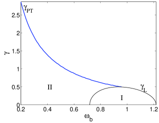
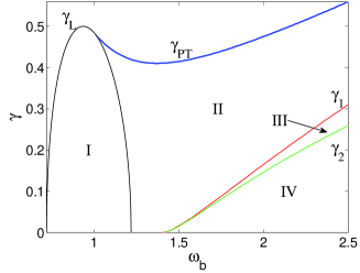
$\epsilon=1$, $\delta=3\epsilon/2$	$\epsilon=-1$, $\delta=3\epsilon/2$
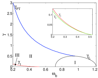
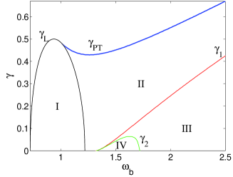
$\epsilon=1$, $\delta=3\epsilon$	$\epsilon=-1$, $\delta=3\epsilon$

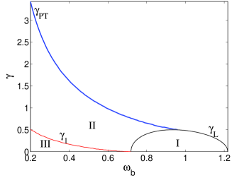
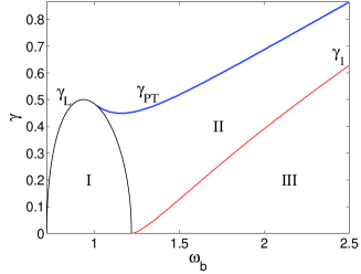
Figure 1: $\gamma$-$\omega_{b}$ plane for $k=\sqrt{15}/8$. Details on the meaning of each curve and region can be found in the text. The linear limit of the oscillator system is denoted by $\gamma_{L}$, while the upper $\mathcal{PT}$-symmetric threshold of solution existence is denoted by $\gamma_{\mathcal{PT}}$. An additional delimiter of the existence of further solutions $\mathrm{A}_{\mathrm{\phi}}$ and $\mathrm{S}_{\mathrm{\phi}}$ is also given by $\gamma_{1}$. The existence regions of the different solutions are encompassed by these curves both in the soft $\epsilon=1$ case (left panels) and in the hard $\epsilon=-1$ case (right panels).

We show below the properties of the $\mathrm{A}_{\mathrm{0}}$, $\mathrm{S}_{\mathrm{0}}$, $\mathrm{A}_{\mathrm{\phi}}$ and $\mathrm{S}_{\mathrm{\phi}}$ solutions in the cases $\delta=\epsilon$, $\delta=3\epsilon/2$ and $\delta=3\epsilon$ for both soft ($\epsilon=+1$) and hard ($\epsilon=-1$) potentials. A summary of the existence and stability regions is displayed in Fig. 1, where the panels depict the $\gamma$-$\omega_{\mathrm{b}}$ planes. Notice that although $\mathrm{A}_{\mathrm{0}}$, $\mathrm{S}_{\mathrm{0}}$, $\mathrm{A}_{\mathrm{\phi}}$ and $\mathrm{S}_{\mathrm{\phi}}$ solutions are, strictly speaking, defined only at $\gamma=0$, we will use this notation for solutions at $\gamma\neq 0$ that are obtained by continuation from the Hamiltonian ($\gamma=0$) limit.

Prior to starting the analysis for arbitrary $\gamma$, we will briefly show the properties of the asymmetric solutions at $\gamma=0$. As explained above, we will choose $k=\sqrt{15}/8$. Notice that for this parameter value, $\omega_{\mathrm{AS+}}^{2}<0$ if $\delta=3\epsilon/2>0$ and consequently, there is no asymmetric solution for this regime. However, there are asymmetric solutions if $\delta=3\epsilon/2<0$ and $\omega_{\mathrm{b}}>\omega_{\mathrm{AS-}}\approx 1.7136$. In fact, at $\omega_{\mathrm{b}}=\omega_{\mathrm{AS-}}$ there is a pitchfork bifurcation, as the $\mathrm{S}_{\mathrm{0}}$ solution is unstable for $\omega_{\mathrm{b}}<\omega_{\mathrm{AS-}}$ and becomes stable past the bifurcation point, where a pair of branches corresponding to unstable asymmetric solutions emerge. For $\delta=3\epsilon$, the situation is similar in the hard case in what regards the existence of solutions (now $\omega_{\mathrm{AS-}}=\omega_{\mathrm{A}}\approx 1.2182$); for the soft case, the asymmetric solution exists for $\omega_{\mathrm{b}}\leq\omega_{\mathrm{AS+}}=\omega_{\mathrm{S}}\approx 0.7182$ and bifurcates from the $\mathrm{A}_{\mathrm{0}}$ solution. Notice that the $\mathrm{A}_{\mathrm{0}}$ (for the soft case) and the $\mathrm{S}_{\mathrm{0}}$ (for the hard case) are all stable; furthermore, the AS solution appears to be marginally stable and highly degenerate as all the eigenfrequencies $\Omega$ are equal to zero; recall also the special, completely integrable nature of this special limit.

We analyze now the properties of the soft potential when $\gamma\neq 0$. In the $\delta=\epsilon$ case, there are two main regions: in region I, only $\mathrm{A}_{\mathrm{0}}$ solutions exist, as $\mathrm{S}_{\mathrm{0}}$ solutions bifurcate from the left arm of the $\gamma_{\mathrm{L}}(\omega_{\mathrm{b}})$ curve (i.e. $\omega_{+}$), which corresponds to the symmetric linear modes; at the right of region I, no solutions are found because $\mathrm{A}_{\mathrm{0}}$ solutions bifurcate from the right arm (i.e. $\omega_{-}$) of the linear dispersion relation. In this soft case of $\epsilon>0$, the bifurcations occur to the left of $\gamma_{\mathrm{L}}(\omega_{\mathrm{b}})$, whereas in the hard case of $\epsilon<0$, they arise to the right of $\gamma_{\mathrm{L}}(\omega_{\mathrm{b}})$. It is easy to show that from (2), $\gamma_{\mathrm{L}}$ is given by:

$$\gamma_{\mathrm{L}}(\omega_{\mathrm{b}})=\frac{\sqrt{(k^{2}-1)+2\omega_{\mathrm{b}}^{2}-\omega_{\mathrm{b}}^{4}}}{\omega_{\mathrm{b}}}.$$ (34)

Consequently, region I is bounded between $\omega_{\mathrm{b}}=\omega_{\mathrm{S}}\approx 0.7182$, $\omega_{\mathrm{b}}=\omega_{\mathrm{A}}\approx 1.2182$ and $\gamma=\gamma_{PT,L}=0.5$. In region II, both $\mathrm{A}_{\mathrm{0}}$ and $\mathrm{S}_{\mathrm{0}}$ solutions exist, and experience the $\mathcal{P}\mathcal{T}$ phase transition at the curve designated as $\gamma_{\mathrm{PT}}(\omega_{\mathrm{b}})$. Notice also that all the solutions existing in both regions I and II are stable. In addition, $\mathrm{A}_{\mathrm{\phi}}$ and $\mathrm{S}_{\mathrm{\phi}}$ solutions can only be found for $\omega_{\mathrm{b}}<\omega_{\mathrm{\phi+}}$, but their existence range is quite small as $\omega_{\mathrm{\phi+}}\approx 0.1782$ and only exist for $\gamma<0.1$.

For $\delta=3\epsilon/2$, both regions I and II have the same properties as before. In addition, region III is included, which is below the curve $\gamma_{1}(\omega_{\mathrm{b}})$. In that region, all four solutions exist and are stable except for $\mathrm{A}_{\mathrm{0}}$. This solution becomes stable only nearby i.e. between the curves $\gamma_{2}(\omega_{\mathrm{b}})$ and $\gamma_{1}(\omega_{\mathrm{b}})$. This small stability region can be observed between red and green curves of the inset of the corresponding panel (notice that this phenomenon was also observed in the $\delta=\epsilon$ case, but was not showcased due to the very small range of existence of $\mathrm{S}_{\mathrm{\phi}}$ and $\mathrm{A}_{\mathrm{\phi}}$ solutions therein). In region II only two solutions exist; for $\omega_{\mathrm{b}}<\omega_{\mathrm{\phi+}}\approx 0.5233$, i.e. above the curve $\gamma_{1}(\omega_{\mathrm{b}})$, $\mathrm{S}_{\mathrm{0}}$ and $\mathrm{S}_{\mathrm{\phi}}$ solutions coexist and collide/disappear at $\gamma_{\mathrm{PT}}(\omega_{\mathrm{b}})$, whereas for $\omega_{\mathrm{b}}>\omega_{\mathrm{\phi+}}$, the coexisting solutions are $\mathrm{A}_{\mathrm{0}}$ and $\mathrm{S}_{\mathrm{0}}$. As a side comment, the reason for the existence of $\mathrm{S}_{\mathrm{\phi}}$ for $\omega_{\mathrm{b}}<\omega_{\mathrm{\phi+}}$ and of $\mathrm{A}_{\mathrm{0}}$ for $\omega_{\mathrm{b}}>\omega_{\mathrm{\phi+}}$ within Region II has to do with the fact that these solutions effectively “morph” from one to the other (smoothly) as this frequency is crossed.

For $\delta=3\epsilon$, the scenario is similar to the last one, except for two points: first, the $\gamma_{1}$ curve finishes at $\omega_{\mathrm{b}}=\omega_{\mathrm{S}}$ and encompasses an accordingly broader region III; and second, the solutions in region III, $\mathrm{A}_{\mathrm{0}}$ and $\mathrm{A}_{\mathrm{\phi}}$, are stable for any value of $\gamma$ and $\omega_{\mathrm{b}}$.

We focus now on the hard potential (i.e. $\epsilon=-1$) properties. In all the cases, we can find the region I, with the same properties as in the soft case (although now it is the $\mathrm{S}_{\mathrm{0}}$ solution that exists and the $\mathrm{A}_{\mathrm{0}}$ that bifurcates into existence beyond the boundary of the region). In addition, region II is present in every case, enclosed between curves $\gamma_{\mathrm{PT}}(\omega_{\mathrm{b}})$ and $\gamma_{1}(\omega_{\mathrm{b}})$; there are two solutions therein: the $\mathrm{A}_{\mathrm{0}}$ solution and the $\mathrm{S}_{\mathrm{0}}$ for $\omega_{\mathrm{b}}<\omega_{\mathrm{\phi-}}$ and the $\mathrm{A}_{\mathrm{0}}$ and $\mathrm{A}_{\mathrm{\phi}}$ for $\omega_{\mathrm{b}}>\omega_{\mathrm{\phi-}}$. Under the curve $\gamma_{1}(\omega_{\mathrm{b}})$, whose minimum value takes place at $\omega_{\mathrm{b}}=\omega_{\mathrm{\phi-}}$ (so that $\omega_{\mathrm{\phi-}}=\omega_{\mathrm{A}}$ for $\delta=3\epsilon$), the four kinds of solutions coexist, so that $\mathrm{S}_{\mathrm{0}}$ and $\mathrm{S}_{\mathrm{\phi}}$ collide and disappear at this line. As in the soft case, there is a “morphing” from the $\mathrm{S}_{\mathrm{0}}$ to $\mathrm{A}_{\mathrm{\phi}}$ solutions when the frequency $\omega_{\mathrm{\phi-}}$ is crossed.

Thus, the most significant difference between the three considered regimes lies in the existence of region IV and curve $\gamma_{2}(\omega_{\mathrm{b}})$. Region III is characterized by the fact that all the solutions exist (as mentioned above) and are stable. However, below the curve $\gamma_{2}(\omega_{\mathrm{b}})$ (i.e. in region IV), solution $\mathrm{S}_{\mathrm{0}}$ becomes unstable. Notice that for $\delta=\epsilon$ this region exists for every $\omega_{\mathrm{b}}>\omega_{\mathrm{\phi-}}\approx 1.4029$. However, if $\delta=3\epsilon/2$, region IV is shrunk to the range $\omega_{\mathrm{\phi-}}\approx 1.3138<\omega_{\mathrm{b}}\lesssim 1.71$. Finally, region IV has totally vanished at $\delta=3\epsilon$.

IV Analysis of the oscillator dimer

In this section, we complete the description of the system by returning to the original oscillator system and analyzing its exact periodic orbits (that up to now we had only approximated using the RWA). This is done by numerically solving in the Fourier space the dynamical equations set (II) [cf. Appendix A]. That is, we express the solution in the form:

$$u(t)=\sum_{n}y_{n}\exp(\mathrm{i}n\omega_{\mathrm{b}}t),\qquad v(t)=\sum_{n}z_{n}\exp(\mathrm{i}n\omega_{\mathrm{b}}t).$$ (35)

We have considered the same cases as in Section III, namely, $\delta/\epsilon$ equal to 1, $3/2$ and 3, with $\epsilon=\pm 1$.

Prior to showing the results, we want to remark that the Fourier coefficients of $\mathrm{S}_{\mathrm{0}}$ and $\mathrm{A}_{\mathrm{0}}$ solutions (due to their symmetry) have the following property:

$$y_{n}=z_{n}^{*}\ \textrm{($\mathrm{S}_{\mathrm{0}}$)},\qquad y_{n}=-z_{n}^{*}\ \textrm{($\mathrm{A}_{\mathrm{0}}$)}.$$ (36)

In what follows, we will first show the properties of the solutions at the Hamiltonian limit $\gamma=0$. Afterwards, we will be focusing in the different cases of $\delta/\epsilon>0$ for $\gamma\neq 0$. In most cases, results will be compared with the previously found results for the RWA.

IV.1 Solutions for $\gamma=0$

We start by analyzing the modes that can be expressed analytically at the $\gamma=0$ limit. In fact, these can be expressed in terms of Jacobi elliptic functions. If $\epsilon>0$ (soft potential), the solutions are of the form:

$$u(t)=A\ {\rm sn}[\beta\ t;m]\,,\quad v(t)=\pm A\ {\rm sn}[\beta\ t;m]\,,$$ (37)

with

$$A=\beta\sqrt{\frac{2m}{\epsilon+\delta}},\,~{}~{}~{}\beta^{2}=\frac{1\mp k}{1+m},\ ~{}~{}~{}\omega_{\mathrm{b}}=\frac{\pi\beta}{2K(m)}.$$ (38)

with the upper (lower) sign corresponding to the $\mathrm{S}_{\mathrm{0}}$ ($\mathrm{A}_{\mathrm{0}}$) solution, $K(m)$ the complete elliptic integral of the first kind with modulus $m$ , and $0<m<1$. As $K(m)>\pi/2$, it is easy to deduce that $\omega_{\mathrm{b}}<\omega_{S}=\sqrt{1-k}$ for the $\mathrm{S}_{\mathrm{0}}$ solution and $\omega_{\mathrm{b}}<\omega_{A}=\sqrt{1+k}$ for the $\mathrm{A}_{\mathrm{0}}$ solution, as within the RWA.

If $\epsilon<0$ (hard potential), these modes can be expressed as:

$$u(t)=A\ {\rm cn}[\beta\ t;m]\,,\quad v(t)=\pm A\ {\rm cn}[\beta\ t;m]\,,$$ (39)

with

$$A=\beta\sqrt{-\frac{2m}{\epsilon+\delta}},\,~{}~{}~{}\beta^{2}=\frac{1\mp k}{1-2m},\ ~{}~{}~{}\omega_{\mathrm{b}}=\frac{\pi\beta}{2K(m)},$$ (40)

where $0<m<1/2$. Similar to the soft case, $\omega_{\mathrm{b}}>\omega_{S}$ for the $\mathrm{S}_{\mathrm{0}}$ solution and $\omega_{\mathrm{b}}>\omega_{\mathrm{A}}$ for the $\mathrm{A}_{\mathrm{0}}$ solution. Notice that for these solutions to exist $\delta<-\epsilon$.

At $\delta=\epsilon$ and for a hard potential, the $\mathrm{S}_{\mathrm{\phi}}$ and $\mathrm{A}_{\mathrm{\phi}}$ solutions are given by:

$$u(t)=A{\rm sn}(\beta t;m)+B\sqrt{m}{\rm cn}(\beta t;m)\,,\quad~{}~{}v(t)=\pm[A\sqrt{m}{\rm sn}(\beta t;m)-B\sqrt{m}{\rm cn}(\beta t;m)]\,,$$ (41)

provided

$$A=\sqrt{\frac{(3m-2)\beta^{2}+2}{4\epsilon}},\,B=\sqrt{\frac{1-(2m+1)\beta^{2}}{2\epsilon}},\,\beta^{2}=2k/m,\ ~{}~{}~{}\omega_{\mathrm{b}}=\frac{\pi\beta}{2K(m)}.$$ (42)

The AS solution can be analytically expressed whenever $\delta=3\epsilon$. If $\epsilon>0$, it is given by:

$$u(t)=A_{+}\ {\rm sn}[\beta_{+}\ t;m_{+}]+A_{-}\ {\rm sn}[\beta_{-}\ t;m_{-}]\,,\quad v(t)=A_{+}\ {\rm sn}[\beta_{+}\ t;m_{+}]-A_{-}\ {\rm sn}[\beta_{-}\ t;m_{-}]\,,$$ (43)

with

$$A_{\pm}=\beta_{\pm}\sqrt{\frac{2m_{\pm}}{\epsilon}},\,~{}~{}~{}\beta_{\pm}^{2}=\frac{1\mp k}{1+m_{\pm}},\ ~{}~{}~{}\omega_{\mathrm{b}}=\frac{\pi\beta_{+}}{2K(m_{+})}=\frac{\pi\beta_{-}}{2K(m_{-})},\,$$ (44)

whereas if $\epsilon<0$, the AS solution is:

$$u(t)=A_{+}\ {\rm cn}[\beta_{+}\ t;m_{+}]+A_{-}\ {\rm cn}[\beta_{-}\ t;m_{-}]\,,\quad v(t)=A_{+}\ {\rm cn}[\beta_{+}\ t;m_{+}]-A_{-}\ {\rm cn}[\beta_{-}\ t;m_{-}]\,,$$ (45)

with

$$A_{\pm}=\beta_{\pm}\sqrt{-\frac{2m_{\pm}}{\epsilon}},\,~{}~{}~{}\beta_{\pm}^{2}=\frac{1\mp k}{1-2m_{\pm}},\ ~{}~{}~{}\omega_{\mathrm{b}}=\frac{\pi\beta_{+}}{2K(m_{+})}=\frac{\pi\beta_{-}}{2K(m_{-})},\,.$$ (46)

It can be numerically observed that $\mathrm{A}_{\mathrm{0}}$, $\mathrm{S}_{\mathrm{0}}$ and AS solutions exist for every $\delta$ whereas $\mathrm{A}_{\mathrm{\phi}}$ and $\mathrm{S}_{\mathrm{\phi}}$ do not exist for $\delta\leq 3\epsilon/2$ in the $\epsilon=+1$ case. On the contrary, a new solution denoted as $\mathrm{A}_{\mathrm{3}}$ exists for the soft potential and all of the considered values of $\delta$; this new solution, which was not found in the $\delta=0$ case, is characterized by a high increase of the third harmonic in the Fourier series, and, consequently, cannot be predicted by the RWA. The existence of this new solution can be caused by the hybridization of the $\mathrm{S}_{\mathrm{0}}$ mode with frequency $\omega_{\mathrm{b}}$ and the $\mathrm{A}_{\mathrm{0}}$ mode with frequency $3\omega_{\mathrm{b}}$; this symmetry breaking effect could happen whenever $\omega_{\mathrm{b}}<\omega_{\mathrm{A}}/3\approx 0.4061$. Notice that the $\mathrm{A}_{\mathrm{3}}$ mode bifurcates from the $\mathrm{S}_{\mathrm{0}}$ mode at $\omega_{3}$, which exactly coincides with $\omega_{\mathrm{A}}/3$ when $\delta=3\epsilon$, but is smaller than this when $\delta<3\epsilon$ (e.g. for $\delta=3\epsilon/2$, $\omega_{3}\approx 0.384$ whereas $\omega_{3}\approx 0.365$ for $\delta=\epsilon$.). There is no stability change at this bifurcation.

The asymmetric (AS) solution preserves the properties of the RWA. That is, it bifurcates from the $\mathrm{A}_{\mathrm{0}}$ solution in soft potentials and from the $\mathrm{S}_{\mathrm{0}}$ solution for hard potentials. The AS solution does not exist for $\epsilon=\delta$ and for $\delta=3\epsilon/2>0$. Besides, all the Floquet exponents are $\theta=0$ (or, equivalently, the Floquet multipliers are $+1$) for $\delta=3\epsilon$. For $\delta=3\epsilon/2<0$, the AS solution is unstable, as in the RWA. In addition, for $\delta=3\epsilon$, the AS, $\mathrm{S}_{\mathrm{\phi}}$ and $\mathrm{A}_{\mathrm{\phi}}$ solutions bifurcate from the $\mathrm{A}_{\mathrm{0}}$ solution at $\omega_{\mathrm{b}}=\omega_{\mathrm{S}}$ if $\epsilon=+1$, with the $\mathrm{S}_{\mathrm{\phi}}$ and $\mathrm{A}_{\mathrm{\phi}}$ solutions being stable and the $\mathrm{A}_{\mathrm{0}}$ stable (unstable) for $\omega_{\mathrm{b}}>\omega_{\mathrm{S}}$ ($\omega_{\mathrm{b}}<\omega_{\mathrm{S}}$); if $\epsilon=-1$, the AS, $\mathrm{S}_{\mathrm{\phi}}$ and $\mathrm{A}_{\mathrm{\phi}}$ solutions bifurcate from the $\mathrm{S}_{\mathrm{0}}$ mode at $\omega_{\mathrm{b}}=\omega_{\mathrm{A}}$, with the $\mathrm{S}_{\mathrm{0}}$ solution being stable and the $\mathrm{S}_{\mathrm{\phi}}$ unstable, whereas the $\mathrm{A}_{\mathrm{\phi}}$ is marginally stable as are the AS solutions (all the Floquet exponents are zero). In the $\delta=3\epsilon/2<0$ case, the $\mathrm{S}_{\mathrm{\phi}}$ and $\mathrm{A}_{\mathrm{\phi}}$ solutions, which are stable, bifurcate from the $\mathrm{S}_{\mathrm{0}}$ solution at $\omega_{\mathrm{b}}\approx 1.306$ which is close to $\omega_{\mathrm{\phi-}}$; the $\mathrm{S}_{\mathrm{0}}$ solution is stable (unstable) for $\omega_{\mathrm{b}}$ smaller (higher) than the bifurcation point. This latter bifurcation also occurs for $\delta=\epsilon=-1$, taking place in this case at $\omega_{\mathrm{b}}\approx 1.386$. In addition, the AS solution (which is unstable) bifurcates from the $\mathrm{S}_{\mathrm{0}}$ solution (which changes its stability) at $\omega_{\mathrm{b}}\approx 1.708$, a value which is close to (but not exactly at) $\omega_{\mathrm{AS-}}$. We must also mention that for the case analyzed in PRA , i.e. $\delta=0$, the AS solution bifurcates from the $\mathrm{S}_{\mathrm{0}}$ ($\mathrm{A}_{\mathrm{0}}$) solution in the soft (hard) potential. This situation is reversed in the present observations for sufficiently large $\delta\neq 0$, which suggests the existence of a critical point.

Finally, as within the RWA, the energy coincides for the AS, $\mathrm{S}_{\mathrm{\phi}}$ and $\mathrm{A}_{\mathrm{\phi}}$ solutions when $\delta=3\epsilon$.

$\epsilon=1$, $\delta=\epsilon$, $\gamma=0$	$\epsilon=-1$, $\delta=\epsilon$, $\gamma=0$
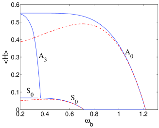
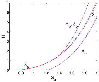
$\epsilon=1$, $\delta=3\epsilon/2$, $\gamma=0$	$\epsilon=-1$, $\delta=3\epsilon/2$, $\gamma=0$
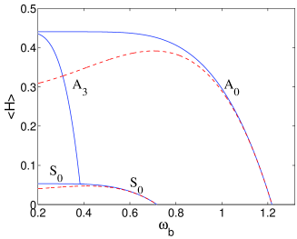
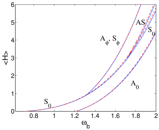
$\epsilon=1$, $\delta=3\epsilon$, $\gamma=0$	$\epsilon=-1$, $\delta=3\epsilon$, $\gamma=0$

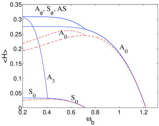
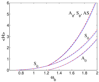
Figure 2: Energy versus $\omega_{\mathrm{b}}$ at $\gamma=0$. Full blue lines correspond to the Hamiltonian (4) of full Klein-Gordon dimer whereas the dashed red lines represent the averaged energy within the RWA (III.1).

All the previous properties are summarized in Fig. 2 where the Hamiltonian energy is depicted versus $\omega_{\mathrm{b}}$ and compared with the averaged Hamiltonian for the RWA. This figure is complemented by Figs. 3 and 4 where the time evolution of the different solutions are displayed. Importantly, we should point out here that it is evident that the approximations involved in the RWA become demonstrably less accurate especially in the soft nonlinearity case and particularly as the frequency $\omega$ decreases away from the linear limit (and hence nonlinear terms become more significant). Nevertheless, the qualitative agreement of the features of Fig. 2 is still fairly satisfactory for the regime of parameters considered herein. On the other hand, for the hard nonlinearity case, the agreement seems to be even quantitatively accurate for the frequency range considered.

$\mathrm{S}_{\mathrm{0}}$ solution	$\mathrm{A}_{\mathrm{0}}$ solution
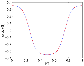
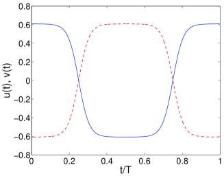
$\mathrm{S}_{\mathrm{\phi}}$ solution	$\mathrm{A}_{\mathrm{\phi}}$ solution
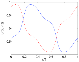
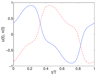
AS solution	$\mathrm{A}_{\mathrm{3}}$ solution

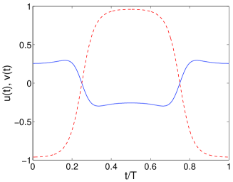
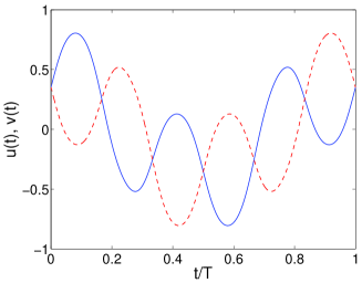
Figure 3: Time evolution of all the different solutions considered at $\delta=3\epsilon$ for the soft nonlinearity case of $\epsilon=1$ and $\omega_{\mathrm{b}}=0.3$; here $\gamma=0$.

$\mathrm{S}_{\mathrm{0}}$ solution	$\mathrm{A}_{\mathrm{0}}$ solution
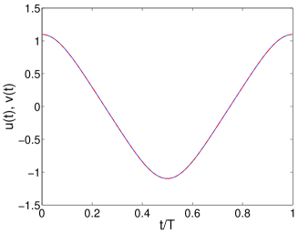
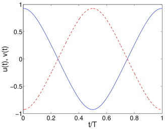
$\mathrm{S}_{\mathrm{\phi}}$ solution	$\mathrm{A}_{\mathrm{\phi}}$ solution
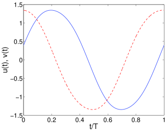
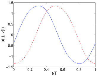
AS solution

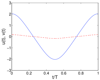
Figure 4: Time evolution of the solutions at $\delta=3\epsilon$ for the hard nonlinearity case of $\epsilon=-1$ and $\omega_{\mathrm{b}}=2$. Again here, $\gamma=0$.

IV.2 $\delta=\epsilon$ case: existence of exact solutions

One of the main features of this case is the existence of two exact periodic solutions to (II):

$$u(t)=A\sin(\omega_{\mathrm{b}}\,t),\qquad v(t)=\pm A\cos(\omega_{\mathrm{b}}\,t)$$ (47)

fulfilling that:

$$k=\mp\gamma\omega_{\mathrm{b}},\ ~{}~{}~{}A=\sqrt{\frac{1-\omega_{b}^{2}}{\epsilon}}\ ,$$ (48)

with the upper sign corresponding to the symmetric solution and the lower one to the anti-symmetric solution. It is important to note that for a given $k$, the frequency is proportional to $1/\gamma$. Thus, the two solutions collide as $\gamma\rightarrow\infty$, when $\omega_{\mathrm{b}}\rightarrow 0$. That is, contrary to the “standard” model of $\delta=0$, since for the case considered herein there exist nonlinear solutions for all values of $\gamma$ that are not subject to the relevant transition . This solution can actually be cast as $y_{n}=z_{n}=0\ \forall|n|>1$ and $\phi=\pm\pi/2$. If we fix the value of $\epsilon$, it is clear from Eq. (48) that the properties of the solutions only depend on two parameters, as $k=k(\omega_{\mathrm{b}},\gamma)$. That is, contrary to what we have discussed so far, here we do not fix $k$ and vary $\gamma$ and $\omega_{\mathrm{b}}$, but rather than varying $\gamma$ and $\omega_{\mathrm{b}}$, we fix a value of $k$ associated with them through Eq. (48). Thus, we will consider the effect on the stability of varying parameters $\omega_{\mathrm{b}}$ and $\gamma$ in the case $\epsilon=1$ (soft potential) and $\epsilon=-1$ (hard potential). Notice also that given the restrictions formulated in (48) and the symmetry properties of the dynamical equations, the Floquet spectrum for a given set of parameters is the same for both solutions.

Fig. 5 shows the stability/instability regions for these solutions. Shaded areas correspond to stable solutions. The black line therein indicates the locus in the $\gamma$-$\omega_{\mathrm{b}}$ plane where $k=\sqrt{15}/8$ (i.e., the value used for other results in the present work). From this line, it can be deduced that solutions with $\phi=\pm\pi/2$ when $\delta=\epsilon$ are stable in the range $\omega_{\mathrm{b}}\in[0.8535,1]$ if $\epsilon=1$ and in $\omega_{\mathrm{b}}\in[1,1.029]\cup[1.2206,\infty)$ if $\epsilon=-1$.

The averaged energy is, for both solutions, $<H>=\frac{1+2\omega^{2}-3\omega^{4}}{3\epsilon}$ which, for $\epsilon=1$ has a maximum at $\omega_{\mathrm{b}}=3^{-1/2}\approx 0.5774$; for $\epsilon=-1$, this function is monotonically decreasing. It is worth mentioning that for $\gamma=0$, where the averaged energy coincides with the Hamiltonian, there is a stability change at $\omega=3^{-1/2}$, the value at which $\partial H/\partial\omega$ changes its slope. This correlation between energy maximum and stability changes, which resembles the Vakhitov-Kolokolov criterion for NLS systems, is not observed for solutions that do not fulfill condition (48) and, consequently, possess more than one harmonic in their Fourier series.

$\delta=\epsilon=+1$, $|\phi|=\pi/2$	$\delta=\epsilon=-1$, $|\phi|=\pi/2$

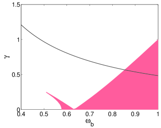
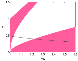
Figure 5: Stability (shaded) and instability (blank) regions for the exact solutions (i.e. those with $\phi=\pm\pi/2$) in the Klein–Gordon dimer arising for $\delta=\epsilon$. The black line corresponds to $k=\sqrt{15}/8$ according to Eq. (48), i.e., the value generally considered throughout the paper.

The above mentioned exact solutions constitute only a subset of the whole $\gamma-\omega_{\mathrm{b}}$ plane, which is depicted in Fig. 6. This figure shows the existence range of the different solutions that arise for $\gamma\neq 0$ and $\delta=\epsilon$. We explain below the different regions and curves.

$\delta=\epsilon=+1$	$\delta=\epsilon=-1$

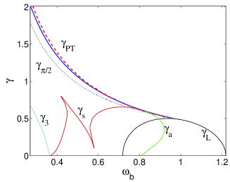
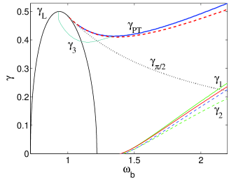
Figure 6: Planes with curves separating regions of solutions that share the same properties when $\epsilon=1$ and $s=\sqrt{15}/8$ (see text). Dashed lines correspond to the RWA predictions and the dotted line $\gamma_{\pi/2}$ corresponds to the exact solutions with phase $\pi/2$ described in Fig. 5. Notice that the colors of the dashed lines are inverted with respect to that of the numerical results for a better visualization. This inversion pattern is followed also in all figures comparing theory and numerical computations from here on.

In the case of soft potential, we observe, as expected, the curve $\gamma_{\mathrm{L}}$ which encloses a region with only $\mathrm{A}_{\mathrm{0}}$ solutions, as $\mathrm{S}_{\mathrm{0}}$ bifurcates from the left arm of the curve. In addition, above the curve $\gamma_{\mathrm{PT}}$, which indicates the $\mathcal{P}\mathcal{T}$ transition and is very close to the value predicted by RWA, there are no periodic orbits. This transition is caused by the collision of $\mathrm{A}_{\mathrm{0}}$ and $\mathrm{S}_{\mathrm{0}}$ solutions whenever $\omega_{\mathrm{b}}>\omega_{3}\approx 0.365$. Contrary to the expectation from RWA, there are three more curves in the considered range. At the right of curve $\gamma_{\mathrm{a}}$, $\mathrm{A}_{\mathrm{0}}$ solutions are stable; similarly, below to the right of the curve denoted by $\gamma_{\mathrm{s}}$, $\mathrm{S}_{\mathrm{0}}$ solutions are stable. Consequently, for $\omega_{\mathrm{b}}\lesssim 0.8$ the $\mathcal{P}\mathcal{T}$ phase transition takes place between the unstable $\mathrm{S}_{\mathrm{0}}$ and $\mathrm{A}_{\mathrm{0}}$ solutions. This behavior is similar to the one observed for the $\delta=0$ case PRA . Notice the existence of a third curve $\gamma_{3}$, which terminates at $\omega_{\mathrm{b}}=\omega_{3}$. This curve corresponds to the loci for the occurrence of the saddle-node bifurcation between the $\mathrm{S}_{\mathrm{0}}$ and $\mathrm{A}_{\mathrm{3}}^{+}$ solutions. With this notation we remark that this solution is a $\mathrm{A}_{\mathrm{3}}$ mode whose phase difference $\varphi$ is in the first quadrant for $\gamma\approx 0$. Remarkably, there is a different behavior regarding $\mathrm{S}_{\mathrm{0}}$ in the regions between the curves $\gamma_{\mathrm{s}}$ and $\gamma_{3}$; in the former, the phase of the mode is in the fourth quadrant whereas in the latter, the phase lies in the first quadrant. Additionally, for $\omega_{\mathrm{b}}<\omega_{3}$, the $\mathrm{A}_{\mathrm{0}}$ mode collides and disappears at $\gamma_{\mathrm{PT}}$ with the $\mathrm{A}_{\mathrm{3}}^{-}$ mode; contrary to the $\mathrm{A}_{\mathrm{3}}^{+}$ case, the phase of this mode lies in the fourth quadrant. Notice also that in the region below curve $\gamma_{3}$, the stability description is not trivial; despite this, we can say that for small $\gamma$, both $\mathrm{A}_{\mathrm{3}}^{+}$ and $\mathrm{S}_{\mathrm{0}}$ solutions are stable. Finally, for $\omega_{\mathrm{b}}\lesssim 0.31$, we observe that both $\mathrm{A}_{\mathrm{3}}$ solutions coalesce into the $\mathrm{A}_{\mathrm{0}}$ solution with frequency $3\omega_{\mathrm{b}}$ and the $\mathrm{S}_{\mathrm{0}}$ solution transforms into a new solution that collides and disappears with the $\mathrm{A}_{\mathrm{0}}$ solution at $\gamma_{\mathrm{PT}}$. A summary of the bifurcations for $\omega_{\mathrm{b}}>\omega_{3}$, together with energy, phases, Floquet multipliers and comparisons with RWA are shown in Fig. 7. Figure 8 shows the bifurcation diagrams and Floquet multipliers for $\omega_{\mathrm{b}}=0.35$ and $\omega_{\mathrm{b}}=0.3$.

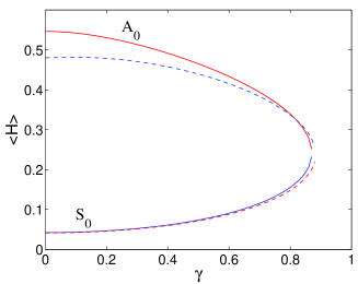
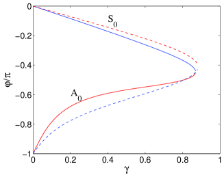
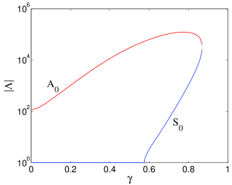
Figure 7: Averaged energy (left), phase difference (center) and modulus of the Floquet multipliers (right) [only the multipliers with moduli higher than one are shown] as a function of the gain/loss parameter $\gamma$ for $\epsilon=\delta=1$, $\omega_{\mathrm{b}}=0.6$, and $s=\sqrt{15}/8$. Notice the logarithmic scale in the $y$-axis of the latter graph. In the left and central panels, blue (red) solid line corresponds to the $\mathrm{S}_{\mathrm{0}}$ ($\mathrm{A}_{\mathrm{0}}$) solution, while red (blue), i.e., reversed colors, dashed lines correspond to the $\mathrm{S}_{\mathrm{0}}$ ($\mathrm{A}_{\mathrm{0}}$) branch from the RWA predictions. The figure on the right does not show the RWA prediction as they only qualitatively match the results for the oscillator dimer for this value of $\omega_{\mathrm{b}}$.

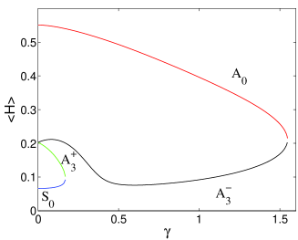
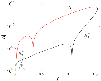
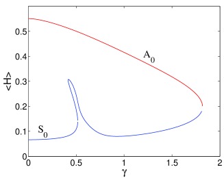
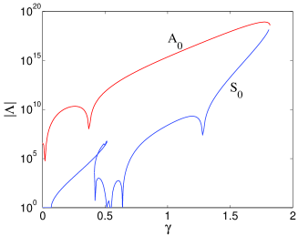
Figure 8: Averaged energy (left) and modulus of the Floquet multipliers (right) as a function of the gain/loss parameter $\gamma$ for $\epsilon=\delta=1$ and $\omega_{\mathrm{b}}=0.35$ (top) or $\omega_{\mathrm{b}}=0.3$ (bottom). Blue (red) line corresponds to the $\mathrm{S}_{\mathrm{0}}$ ($\mathrm{A}_{\mathrm{0}}$) solution, while in the top panels, black and green lines represent the two $\mathrm{A}_{\mathrm{3}}$ solutions discussed in the text, $\mathrm{A}_{\mathrm{3}}^{+}$ and $\mathrm{A}_{\mathrm{3}}^{-}$.

The case of hard potential ($\delta=\epsilon=-1$) is also illustrated in Fig. 6. The curves and regions are equivalent to the RWA case, except for one fact: there is a region between curves $\gamma_{3}$ and $\gamma_{\mathrm{PT}}$ where the $\mathrm{S}_{\mathrm{0}}$ solution is unstable, similar to the $\delta=0$ case PRA . Since this is the only feature not captured by the RWA, it must be directly connected with the emergence/role of higher harmonics in the system. Figure 9 shows the averaged energy, relative phase and Floquet exponents for the different solutions and compares them with the corresponding RWA results for $\omega_{\mathrm{b}}=1.3$ and $\omega_{\mathrm{b}}=2$, identifying accurate semi-quantitative agreement, as expected from the discussion above.

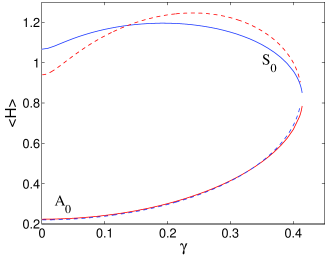
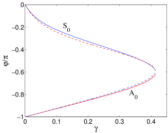
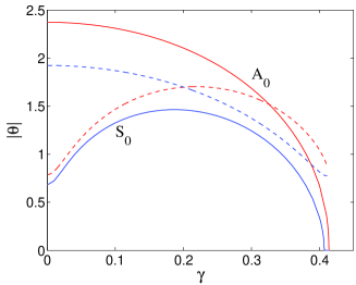
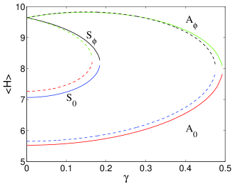
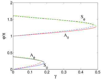
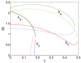
Figure 9: Same as Fig. 7 but for the case $\delta=\epsilon=-1$ and $\omega_{\mathrm{b}}=1.3$ (top) and $\omega_{\mathrm{b}}=2$ (bottom). Notice that, as solutions are mostly stable, the Floquet argument is displayed instead of its modulus.

IV.3 $\delta=3\epsilon/2$ case: Manakov-like coupling

$\delta=3\epsilon/2$. $\epsilon=+1$	$\delta=3\epsilon/2$. $\epsilon=-1$

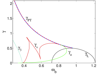
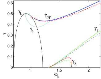
Figure 10: Planes with curves separating regions of solutions that share the same properties when $\delta=3\epsilon/2$ and $s=\sqrt{15}/8$ (see text).

The interest of this case lies in the fact that, in the RWA, the coupling between fields, is similar to the Manakov equation i.e., bearing equal self- and cross- interaction among the complex nonlinear variables $\phi_{1,2}$. Figure 10 shows the different regions for the soft and hard case. In the soft case, the behavior is similar to that of $\delta=\epsilon$, even though the RWA predicted the existence of $\mathrm{A}_{\mathrm{\phi}}$ and $\mathrm{S}_{\mathrm{\phi}}$ solutions for this case. For $\omega_{\mathrm{b}}\lesssim 0.29$, the bifurcation diagram becomes very complex, similar to the $\delta=\epsilon$ case. For the hard case, the phenomenology is similar to the $\delta=\epsilon$ case; i.e. there is a good agreement with the RWA except for an additional region for which the $\mathrm{S}_{\mathrm{0}}$ solution is unstable. Because of the greater similarity with the $\delta=\epsilon$ case, no bifurcation diagrams are included for the present case.

IV.4 $\delta=3\epsilon$ case: Integrability

$\delta=3\epsilon$. $\epsilon=+1$	$\delta=3\epsilon$. $\epsilon=-1$

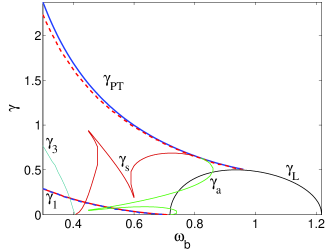
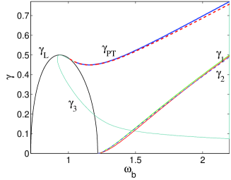
Figure 11: Planes with curves separating regions of solutions that share the same properties when $\delta=3\epsilon$ and $s=\sqrt{15}/8$ (see text).

This case is arguably more interesting than the previous one, not only because of the existence of more solution families and also nontrivial discrepancies with the RWA regimes, but also because of the integrability of the dynamical equations, as they form the Hamiltonian $H_{2}$ [cf. Eq. (5)]

Figure 11 illustrates the different regions in this case. For the soft case, the $\mathrm{A}_{\mathrm{\phi}}$ and $\mathrm{S}_{\mathrm{\phi}}$ modes do exist, as in the RWA. Contrary to the RWA predictions, however, the modes bifurcating at $\gamma_{\mathrm{PT}}$ are the $\mathrm{S}_{\mathrm{0}}$ and $\mathrm{A}_{\mathrm{\phi}}$ ones for $\omega_{\mathrm{b}}>\omega_{3}=\omega_{\mathrm{A}}/3$ and the $\mathrm{A}_{\mathrm{3}}^{-}$ and $\mathrm{A}_{\mathrm{\phi}}$ otherwise, whereas the modes $\mathrm{A}_{\mathrm{0}}$ and $\mathrm{S}_{\mathrm{\phi}}$ bifurcate at $\gamma_{1}$. The curves $\gamma_{\mathrm{s}}$ and $\gamma_{3}$ have a similar meaning as before, whereas at the right of curve $\gamma_{\mathrm{a}}$ it is the $\mathrm{A}_{\mathrm{\phi}}$ mode which is unstable. While the RWA predicted stability for modes below curve $\gamma_{1}$, here the $\mathrm{A}_{\mathrm{0}}$ and $\mathrm{S}_{\mathrm{\phi}}$ modes are stable for small $\gamma$ and unstable close to $\gamma_{1}$ (the change of stability curve is not shown in the figure in order not to make it even more complex).

The hard case is similar to the previous ones except for two facts: (i) the curve $\gamma_{3}$, above which the $\mathrm{S}_{\mathrm{0}}$ mode is unstable, extends now for every value of $\omega_{\mathrm{b}}$, tending asymptotically to $\gamma=0$ for high $\omega_{\mathrm{b}}$ (and, consequently, for $\omega_{\mathrm{b}}>\omega_{\mathrm{A}}$ the $\mathrm{A}_{\mathrm{\phi}}$ solution is unstable above the curve); (ii) below curve $\gamma_{2}$ (which does not exist within the RWA), the $\mathrm{S}_{\mathrm{\phi}}$ solution is unstable, contrary to the previous values of $\delta$ for which it was the $\mathrm{S}_{\mathrm{0}}$ mode that was unstable below the curve.

Figure 12 illustrates the bifurcations mentioned above by means of the dependence of $H_{2}$ on $\gamma$ . From the figure, it is evident that depending on the particular value of the frequency, it is possible that $\mathrm{S}_{\mathrm{0}}$ and $\mathrm{A}_{\mathrm{\phi}}$, as well as $\mathrm{S}_{\mathrm{\phi}}$ and $\mathrm{A}_{\mathrm{0}}$ will collide and disappear in pairwise saddle-center bifurcations (left); or, $\mathrm{A}_{\mathrm{3}}^{+}$ and $\mathrm{S}_{\mathrm{0}}$, as well as $\mathrm{A}_{\mathrm{3}}^{-}$ and $\mathrm{A}_{\mathrm{\phi}}$ may feature such collisions (middle); or $\mathrm{S}_{\mathrm{0}}$ and $\mathrm{S}_{\mathrm{\phi}}$, and $\mathrm{A}_{\mathrm{0}}$ and $\mathrm{A}_{\mathrm{\phi}}$ may collide and disappear hand-in-hand (right panel).

$\delta=3\epsilon$, $\epsilon=1$, $\omega_{\mathrm{b}}=0.6$	$\delta=3\epsilon$, $\epsilon=1$, $\omega_{\mathrm{b}}=0.3$	$\delta=3\epsilon$, $\epsilon=-1$, $\omega_{\mathrm{b}}=2$

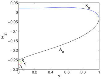
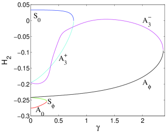
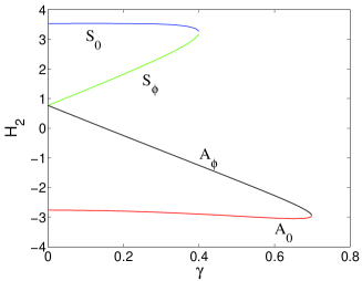
Figure 12: Dependence of $H_{2}$ on $\gamma$ for each mode at different frequencies and $\epsilon$ for the case $\delta=3\epsilon$.

V Dynamics of unstable solutions

Finally, in this section, we briefly touch upon some examples of the dynamical evolution of unstable modes. We are not aiming to be exhaustive; it should be evident at this point that based on the bifurcation scenarios alone, such a detailed study would warrant a separate paper. Instead, we aim to present a few typical examples of dynamical outcomes observed when evolving unstable configurations in this system.

In the soft potential, unstable solutions are mostly prone to blow-up, even in the $\delta=3\epsilon$ case where $H_{2}$ is conserved. This blow-up could consist of both sites tending to $\infty$ or $-\infty$ at the same time (specially in $\mathrm{S}_{\mathrm{0}}$ and $\mathrm{A}_{\mathrm{0}}$ solutions), or one site going to $\infty$ and the other one to $-\infty$ mostly in $\mathrm{A}_{\mathrm{\phi}}$ and $\mathrm{S}_{\mathrm{\phi}}$ solutions. $\mathrm{A}_{\mathrm{0}}$ solutions can exhibit both behaviors. For small values of $\gamma$, the instabilities can lead to quasi-periodic oscillations, whenever the solution at $\gamma=0$ is stable (if the solution is unstable at $\gamma=0$, it is prone to blow-up). Figure 13 shows several examples of the dynamics of soft potentials.

$\delta=\epsilon$, $\epsilon=1$, $\omega_{\mathrm{b}}=0.5$, $\gamma=0.6$ ($\mathrm{S}_{\mathrm{0}}$)	$\delta=\epsilon$, $\epsilon=1$, $\omega_{\mathrm{b}}=0.8$, $\gamma=0.5$ ($\mathrm{A}_{\mathrm{0}}$)
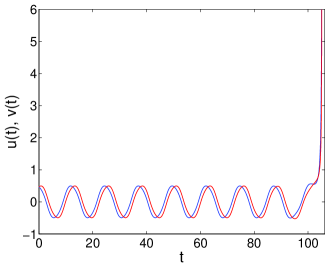
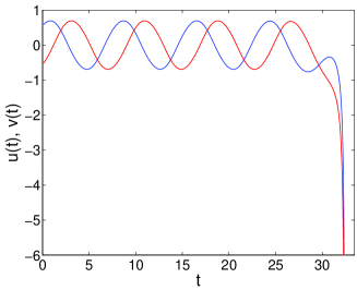
$\delta=3\epsilon$, $\epsilon=1$, $\omega_{\mathrm{b}}=0.5$, $\gamma=0.05$ ($\mathrm{A}_{\mathrm{0}}$)	$\delta=3\epsilon$, $\epsilon=1$, $\omega_{\mathrm{b}}=0.7$, $\gamma=0.02$ ($\mathrm{A}_{\mathrm{\phi}}$)

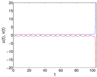
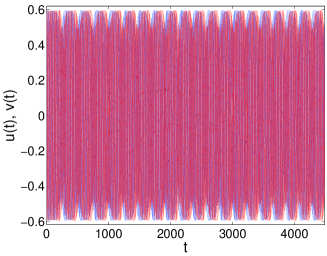
Figure 13: Evolution of unstable solutions for the soft potential. Three examples provide the different combination examples where the oscillator amplitudes may grow indefinitely, while the fourth example presents a bounded apparently quasi-periodic scenario.

In the hard potential case, there are some differences between the dominant behavior when $\delta=\epsilon$ with respect to $\delta=3\epsilon$, as shown in Fig. 14. In the former case, where the instabilities arise from the $\mathrm{S}_{\mathrm{0}}$ solutions, we have observed quasi-periodic oscillations with amplitude peaks when $\omega_{\mathrm{b}}>\omega_{\mathrm{\phi-}}$ and without these peaks if $\omega_{\mathrm{b}}<\omega_{\mathrm{\phi-}}$. In the latter case, although quasi-periodic oscillations are present (mainly for small growth rates), the dominant behavior is an apparent (modulated) exponential growth on the anti-damped site, associated with a decay on the damped site. This decay is very much slower when the instability arises from the $\mathrm{A}_{\mathrm{\phi}}$ solution.

$\delta=\epsilon$, $\epsilon=-1$, $\omega_{\mathrm{b}}=1$, $\gamma=0.16$ ($\mathrm{S}_{\mathrm{0}}$)	$\delta=\epsilon$, $\epsilon=-1$, $\omega_{\mathrm{b}}=2$, $\gamma=0.46$ ($\mathrm{S}_{\mathrm{0}}$)
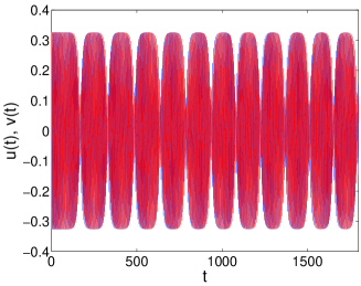
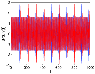
$\delta=3\epsilon$, $\epsilon=1$, $\omega_{\mathrm{b}}=2$, $\gamma=0.2$ ($\mathrm{A}_{\mathrm{\phi}}$)	$\delta=3\epsilon$, $\epsilon=1$, $\omega_{\mathrm{b}}=2$, $\gamma=0.3$ ($\mathrm{S}_{\mathrm{\phi}}$)

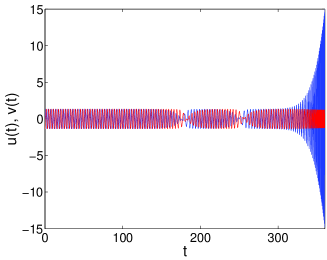
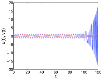
Figure 14: Evolution of unstable solutions for the hard potential. The top panels feature examples of quasi-periodic oscillations, while the bottom panels illustrate indefinite growth of one of the oscillators coupled with a decaying oscillation of the other (possibly very slowly, as in the case of the bottom left panel).

VI Conclusion

In the present work, we have studied various exact solutions and their stability for a generalized $\mathcal{P}\mathcal{T}$-symmetric coupled nonlinear oscillator system. Complementing earlier works both at the linear level bend_gian (describing a recent experiment pt_whisper ) and at the nonlinear level PRA ; bar_gian , we have examined a variety of cases regarding the relative strength of the self- and cross-interaction between our nonlinear oscillators. In our earlier work PRA , only self-interactions were considered, while in the important recent work of bar_gian , only a specific value of the cross interaction was considered ($\delta=3\epsilon$), revealing remarkably the Hamiltonian nature of the model, and then restricting consideration to its DNLS analogue. Here, we have extended considerations to three relevant cases, namely $\delta=\epsilon$, $\delta=3\epsilon/2$ and $\delta=3\epsilon$, exploring how the existence, nonlinear bifurcation and even dynamical trends develop as we move from weaker to stronger cross-interaction between the nonlinear oscillators. Importantly, the relevant pictures were developed not only for the rotating wave approximation model of the DNLS form, but also for the full model of the coupled oscillators. Generally, the two cases, namely the monochromatic approximation and the full system were very similar, except for the highly nonlinear regime, especially in the soft nonlinearity case. Numerous important features were identified along the way including, e.g., new families of solutions at relative phase angles other than $0$ and $\pi$ (introduced by the cross-interaction between oscillators), as well as solutions tractable solely in a numerical form from the four principal families explored. Yet another feature was the existence in the oscillator system of families of solutions not only in the $\gamma=0$ but even in the $\gamma\neq 0$ case in explicit form; one such pair of families appears to “defy” the $\mathcal{P}\mathcal{T}$ phase transition (in the $\delta=\epsilon$ case), existing for all values of the gain/loss parameter $\gamma$. Finally, the instabilities identified in the analysis were monitored in the full dynamics of the system, revealing the possibility of either indefinite growth or that of bounded quasi-periodic oscillations, as the pertinent dynamical outcome.

There are numerous questions that naturally emerge as a result of the present work. Among the most immediate ones, it is worthwhile to extend considerations to the case of, e.g., three oscillators and perhaps even to that of four such, forming effectively a two-dimensional plaquette and a building block for the consideration of higher dimensional systems, in the spirit also of Guenter . Furthermore, here only the case of cubic nonlinearities has been explored, but it might be also of interest, as another prototypical nonlinear system to examine the case of quadratic nonlinearities and how their nonlinear states are “deformed” in the presence of gain and loss. At a perhaps deeper level, however, there are also some intriguing questions that we feel are raised. For one, an apparently $\mathcal{P}\mathcal{T}$-symmetric and viewed as a gain-loss bearing system at $\delta=3\epsilon$ is found to be Hamiltonian. This raises the natural yet difficult question: can we discern such a potential Hamiltonian nature and classify a system as Hamiltonian (and not $\mathcal{P}\mathcal{T}$) possibly through an appropriate (to be identified) transformation? If so, what is the relevant criterion and how can we exclude the presence of a yet-unknown transform that may convert a system classified as $\mathcal{P}\mathcal{T}$ into one which is genuinely Hamiltonian in a different set of variables ? Potential progress along these veins will be reported in future work.

P.G.K. acknowledges support from the National Science Foundation under grants CMMI-1000337, DMS-1312856, from FP7-People under grant IRSES-606096, from the US-AFOSR under grant FA9550-12-10332 and from the Binational (US-Israel) Science Foundation through grant 2010239. This work was supported in part by the U.S. Department of Energy. A.K. acknowledges financial support from Dept. of Atomic Energy, Govt. of India through a Raja Ramanna Fellowship. P.G.K. also acknowledges useful discussions with Igor Barashenkov.

Appendix A Numerical analysis of periodic orbits

In order to calculate periodic orbits, we make use of a Fourier space implementation of the dynamical equations and continuations in frequency or gain/loss parameter are performed via a path-following (Newton-Raphson) method. Fourier space methods are based on the fact that the solutions are $T_{\mathrm{b}}$-periodic; for a detailed explanation of these methods, the reader is referred to Refs. AMM99 ; phason . The method has the advantage, among others, of providing an explicit, analytical form of the Jacobian. Thus, the solution for the two nodes can be expressed in terms of a truncated Fourier series expansion:

$$u(t)=\sum_{n=-n_{m}}^{n_{m}}y_{n}\exp(\mathrm{i}n\omega_{\mathrm{b}}t),\qquad v(t)=\sum_{n=-n_{m}}^{n_{m}}z_{n}\exp(\mathrm{i}n\omega_{\mathrm{b}}t),$$ (49)

with $n_{m}$ being the maximum of the absolute value of the running index $k$ in our Galerkin truncation of the full Fourier series solution. In the numerics, $n_{m}$ has been chosen as 21. After the introduction of (49), the dynamical equations (II) yield a set of $2\times(2n_{m}+1)$ nonlinear, coupled algebraic equations:

$$F_{n,1} \equiv -\omega_{\mathrm{b}}^{2}n^{2}y_{n}-\mathrm{i}\gamma\omega_{\mathrm{b}}ny_{n}+\mathcal{F}_{n}[V^{\prime}(u,v)]-kz_{n}=0,$$ (50)

$$F_{n,2} \equiv -\omega_{\mathrm{b}}^{2}n^{2}z_{n}+\mathrm{i}\gamma\omega_{\mathrm{b}}nz_{n}+\mathcal{F}_{n}[V^{\prime}(v,u)]-ky_{n}=0,$$ (51)

with $V^{\prime}(u_{1},u_{2})=u_{1}-\epsilon u_{1}^{3}-\delta u_{1}u_{2}^{2}$. Here, $\mathcal{F}_{n}$ denotes the Discrete Fourier Transform:

$$\mathcal{F}_{n}[V^{\prime}(u)]=\frac{1}{N}\sum_{q=-n_{m}}^{n_{m}}V^{\prime}\left(\sum_{p=-n_{m}}^{n_{m}}y_{p}\exp\left[\mathrm{i}\frac{2\pi pq}{N}\right]\right)\exp\left[-\mathrm{i}\frac{2\pi nq}{N}\right],$$ (52)

with $N=2n_{m}+1$. The procedure for $\mathcal{F}_{n}(v)$ is similar to the previous case. As $u(t)$ and $v(t)$ must be real functions, it implies that $y_{-n}=y^{*}_{n},\ z_{-n}=z^{*}_{n}$.

In order to study the spectral stability of periodic orbits, we introduce a small perturbation $\{\xi_{1},\xi_{2}\}$ to a given solution $\{u_{0},v_{0}\}$ of Eqs. (II) according to $u=u_{0}+\xi_{1}$, $v=v_{0}+\xi_{2}$. Then, the equations satisfied to first order in $\xi_{n}$ read:

$$\ddot{\xi}_{1} = (3\epsilon u_{0}^{2}+\delta v_{0}^{2}-1)\xi_{1}+\gamma\dot{\xi}_{1}+(k+2\delta u_{0}v_{0})\xi_{2},$$

$$\ddot{\xi}_{2} = (3\epsilon v_{0}^{2}+\delta u_{0}^{2}-1)\xi_{2}-\gamma\dot{\xi}_{2}+(k+2\delta u_{0}v_{0})\xi_{1},$$ (53)

or, in a more compact form: $\mathcal{N}(\{u(t),v(t)\})\xi=0\,$, where $\mathcal{N}(\{u(t),v(t)\})$ is the relevant linearization operator. In order to study the spectral (linear) stability analysis of the relevant solution, a Floquet analysis can be performed if there exists $T_{b}\in\mathbb{R}$ so that the map $\{u(0),v(0)\}\rightarrow\{u(T_{\mathrm{b}}),v(T_{\mathrm{b}})\}$ has a fixed point (which constitutes a periodic orbit of the original system). Then, the stability properties are given by the spectrum of the Floquet operator $\mathcal{M}$ (whose matrix representation is the monodromy) defined as:

$$\left(\begin{array}[]{c}\{\xi_{n}(T_{\mathrm{b}})\}\\ \{\dot{\xi}_{n}(T_{\mathrm{b}})\}\\ \end{array}\right)=\mathcal{M}\left(\begin{array}[]{c}\{\xi_{n}(0)\}\\ \{\dot{\xi}_{n}(0)\}\\ \end{array}\right).$$ (54)

The $4\times 4$ monodromy eigenvalues $\Lambda=\exp(\mathrm{i}\theta)$ are dubbed the Floquet multipliers and $\theta$ are denoted as Floquet exponents (FEs). This operator is real, which implies that there is always a pair of multipliers at $1$ (corresponding to the so-called phase and growth modes) and that the eigenvalues come in pairs $\{\Lambda,\Lambda^{*}\}$. As a consequence, due to the “simplicity” of the FE structure (one pair always at $1$ and one additional pair) there cannot exist Hopf bifurcations in the dimer, as such bifurcations would imply the collision of two pairs of multipliers and the consequent formation of a quadruplet of eigenvalues which is impossible here. Nevertheless, in the present problem, the motion of the pair of multipliers can lead to an instability through exiting (through $1$ or $-1$) on the real line leading to one multiplier (in absolute value) larger than $1$ and one smaller than $1$.

References

- (1) C. M. Bender, Rep. Prog. Phys. 70, 947 (2007).
- (2) See special issues: H. Geyer, D. Heiss, and M. Znojil, Eds., J. Phys. A: Math. Gen. 39, Special Issue Dedicated to the Physics of Non-Hermitian Operators (PHHQP IV) (University of Stellenbosch, South Africa, 2005) (2006); A. Fring, H. Jones, and M. Znojil, Eds., J. Math. Phys. A: Math Theor. 41, Papers Dedicated to the Subject of the 6th International Workshop on Pseudo-Hermitian Hamiltonians in Quantum Physics (PHHQPVI) (City University London, UK, 2007) (2008); C.M. Bender, A. Fring, U. Günther, and H. Jones, Eds., Special Issue: Quantum Physics with non-Hermitian Operators, J. Math. Phys. A: Math Theor. 41, No. 44 (2012).
- (3) K. G. Makris, R. El-Ganainy, D. N. Christodoulides, and Z. H. Musslimani, PT symmetric periodic optical potentials, Int. J. Theor. Phys. 50, 1019 (2011).
- (4) A. Ruschhaupt, F. Delgado, and J. G. Muga, J. Phys. A: Math. Gen. 38, L171 (2005).
- (5) K. G. Makris, R. El-Ganainy, D. N. Christodoulides, and Z. H. Musslimani, Phys. Rev. Lett. 100, 103904 (2008); S. Klaiman, U. Günther, and N. Moiseyev, ibid. 101, 080402 (2008); O. Bendix, R. Fleischmann, T. Kottos, and B. Shapiro, ibid. 103, 030402 (2009); S. Longhi, ibid. 103, 123601 (2009); Phys. Rev. B 80, 235102 (2009); Phys. Rev. A 81, 022102 (2010).
- (6) A. Guo, G. J. Salamo, D. Duchesne, R. Morandotti, M. Volatier-Ravat, V. Aimez, G. A. Siviloglou, and D. N. Christodoulides, Phys. Rev. Lett. 103, 093902 (2009); C. E. Rüter, K. G. Makris, R. El-Ganainy, D. N. Christodoulides, M. Segev, and D. Kip, Nature Phys. 6, 192 (2010); A. Regensburger, C. Bersch, M.-A. Miri, G. Onishchukov, D. N. Christodoulides, and U. Peschel, Nature 488, 167 (2012).
- (7) S.V. Dmitriev, A.A. Sukhorukov, and Yu.S. Kivshar, Opt. Lett. 35, 2976 (2010).
- (8) K. Li and P.G. Kevrekidis, Phys. Rev. E 83, 066608 (2011).
- (9) K. Li, P.G. Kevrekidis, B.A. Malomed, and U. Günther, J. Phys. A Math. Theor. 45, 444021 (2012).
- (10) H. Ramezani, T. Kottos, R. El-Ganainy, and D.N. Christodoulides, Phys. Rev. A 82, 043803 (2010).
- (11) S.V. Suchkov, B.A. Malomed, S.V. Dmitriev, and Yu.S. Kivshar, Phys. Rev. E 84, 046609 (2011).
- (12) A.A. Sukhorukov, Z. Xu, and Yu.S. Kivshar, Phys. Rev. A 82, 043818 (2010).
- (13) D.A. Zezyulin and V.V. Konotop, Phys. Rev. Lett. 108, 213906 (2012).
- (14) A.E. Miroshnichenko, B.A. Malomed, and Yu.S. Kivshar, Phys. Rev. A 84, 012123 (2011)
- (15) H. Cartarius and G. Wunner, Phys. Rev. A 86, 013612 (2012)
- (16) V.V. Konotop, D.E. Pelinovsky, and D.A. Zezyulin, EPL 100, 56006 (2012).
- (17) A.A. Sukhorukov, S.V. Dmitriev, S.V. Suchkov, and Yu.S. Kivshar, Opt. Lett. 37, 2148 (2012).
- (18) M.C. Zheng, D.N. Christodoulides, R. Fleischmann, and T. Kottos, Phys. Rev. A 82, 010103(R) (2010).
- (19) C. M. Bender, B. Berntson, D. Parker, and E. Samuel Am. J. Phys. 81, 173 (2013).
- (20) J. Schindler, A. Li, M.C. Zheng, F.M. Ellis, and T. Kottos, Phys. Rev. A 84, 040101 (2011).
- (21) J. Schindler, Z. Lin, J. M. Lee, H. Ramezani, F. M. Ellis, and T. Kottos, J. Phys. A: Math. Theor. 45, 444029 (2012).
- (22) B. Peng, S.K. Ozdemir, F. Lei, F. Monifi, M. Gianfreda, G.L. Long, S. Fan, F. Nori, C.M. Bender, L. Yang, Nature Physics 10 (2014) 394.
- (23) N. Lazarides, G.P. Tsironis, Phys. Rev. Lett. 110, 053901 (2013). G.P. Tsironis, N. Lazarides Appl. Phys. A 115, 449 (2014).
- (24) N. Bender, S. Factor, J. D. Bodyfelt, H. Ramezani, D. N. Christodoulides, F. M. Ellis, and T. Kottos Phys. Rev. Lett. 110, 234101 (2013).
- (25) C.M. Bender, M. Gianfreda, S.K. Özdemir, B. Peng and L. Yang, Phys. Rev. A 88, 062111 (2013).
- (26) I.V. Barashenkov and M. Gianfreda, J. Phys. A: Math. Theor. 47 282001 (2014).
- (27) J. Cuevas, P.G. Kevrekidis, A. Saxena, and A. Khare, Phys. Rev. A 88, 032108 (2013).
- (28) E.-M. Graefe, J. Phys. A: Math. Theor. 45, 444015 (2012).
- (29) J. Pickton, H. Susanto, Phys. Rev. A 88, 063840 (2013).
- (30) A.S. Rodrigues, K. Li, V. Achilleos, P.G. Kevrekidis, D.J. Frantzeskakis, and C.M. Bender, Romanian Rep. Phys. 65, 5 (2013).
- (31) I.V. Barashenkov, G.S. Jackson and S. Flach, Phys. Rev. A 88, 053817 (2013).
- (32) S.V. Manakov, Sov. Phys. JETP 38, 248 (1974).
- (33) Yu.S. Kivshar and M. Peyrard. Phys. Rev. A 46, 3198 (1992).
- (34) K.W. Sandusky, J.B. Page, and K.E. Schmidt. Phys. Rev. B 46, 6161 (1992).
- (35) J.F.R. Archilla, R.S. MacKay, and J.L. Marín, Physica D 134, 406 (1999).
- (36) J. Cuevas, J.F.R. Archilla, and F.R. Romero, J. Phys. A: Math. Theor. 44, 035102 (2011).