Bayesian Inference for Tumor Subclones Accounting for Sequencing and Structural Variants

Abstract

Tumor samples are heterogeneous. They consist of different subclones that are characterized by differences in DNA nucleotide sequences and copy numbers on multiple loci. Heterogeneity can be measured through the identification of the subclonal copy number and sequence at a selected set of loci. Understanding that the accurate identification of variant allele fractions greatly depends on a precise determination of copy numbers, we develop a Bayesian feature allocation model for jointly calling subclonal copy numbers and the corresponding allele sequences for the same loci. The proposed method utilizes three random matrices, $\bm{L}$, $\bm{Z}$ and $\bm{w}$ to represent subclonal copy numbers ($\bm{L}$), numbers of subclonal variant alleles ($\bm{Z}$) and cellular fractions of subclones in samples ($\bm{w}$), respectively. The unknown number of subclones implies a random number of columns for these matrices. We use next-generation sequencing data to estimate the subclonal structures through inference on these three matrices. Using simulation studies and a real data analysis, we demonstrate how posterior inference on the subclonal structure is enhanced with the joint modeling of both structure and sequencing variants on subclonal genomes. Software is available at http://compgenome.org/BayClone2.

Keywords:   Categorical Indian buffet process; Feature allocation models; Markov chain Monte Carlo; Next-generation sequencing; Random matrices; Subclone; Variant Calling.

1 Introduction

1.1 Biological background and motivation

Understanding tumor heterogeneity (TH) is critical for precise cancer prognosis. Not all tumor cells have the same genome and respond to the same treatment. TH arises when somatic mutations occur in only a fraction of tumor cells, and results in the observed spatial and temporal heterogeneity of tumor samples (Russnes et al., 2011; Greaves and Maley, 2012; Frank and Nowak, 2004; Biesecker and Spinner, 2013; Frank and Nowak, 2003; De, 2011; Bedard et al., 2013; Navin et al., 2011; Ding et al., 2012). In other words, a tumor sample is composed of different subclones of cells with each subclone being defined by a unique genome. Figure 1(a) illustrates this process with a hypothetical case in which accumulation of variants over the lifetime of a tumor gives rise to different subpopulations of tumor cells. Researchers have recently started to recognize the importance of TH and realize the mistake of treating cancer using a “one-size-fits-all” approach. Instead, precision medicine now aims to focus on targeted treatment of individual tumors based on their molecular characteristics, including TH.

Rapid progress has been made in the development of computational tools for clonal inference in the past year (Oesper et al., 2013; Miller et al., 2014; Strino et al., 2013; Jiao et al., 2014; Zare et al., 2014). New methods continue to set new and higher standards in the statistical inference for TH that mimic the underlying biology ever more closely. However, the current literature still lacks effective methods, computational or experimental, for assessing differences between subclonal genomes in terms of both structure variants, such as copy number variants (CNVs), and in terms of sequence variants, such as single nucleotide variants (SNVs). More importantly, current methods lack computational models that could jointly estimate copy numbers and variant allele counts within each subclone. Recent work by Li and Li (2014) adjusts the estimation of subclonal cellular fractions for both CNVs and SNVs, but still stops short of directly inferring subclonal copy numbers or variant allele counts.

Figure 1(b) shows a stylized example of DNA-Seq data for a sample taken on day 360 of the process shown in Figure 1(a). The sample is a result of the underlying tumor evolution. The sample has three tumor subclones. If the sample is sequenced and short reads are mapped, the total number of reads mapped to each locus will be affected by the copy numbers of all the subclones. In Figure 1(b), due to the copy number gains in subclones 2 and 3, we expect that there will be additional reads with sequence A at locus 1 and additional reads with sequence G at locus 3 (both marked by brown letters). In addition, (a) (b) Figure 1: (a) Tumor heterogeneity caused by clonal expansion. On days 90, 180, and 360, four somatic mutations (represented by red letters) and three somatic copy number gains (represented by brown letters) result in three tumor subclones. (b) Observed short reads (some with variants) are results of heterogeneous subclonal genomes. In particular, the formula at the bottom shows that subclonal alleles are mixed in proportions to produce short reads, which are mapped to different loci.    
Figure 2: Three matrices for inference to describe the subclonal structure in Figure 1. $\bm{L}$ describes the subclonal copy numbers, $\bm{Z}$ describes the numbers of subclonal variant alleles, and $\bm{w}$ describes the cellular fractions of subclones.

variant short reads will be generated due to the subclonal mutations in the sample, such as short reads with the red letters mapped to loci 1 and 2. Using NGS data we aim to recover the subclonal sequences at these loci and cellular fractions at the bottom of Figure 1(b) that explains the true biology in (a). In particular, we aim to provide three matrices as shown in Figure 2 to describe the subclonal genomes and sample heterogeneity. For illustration, Figure 2 fills in the (biological) truth for these three matrices corresponding to the hypothetical tumor heterogeneity described in Figure 1(a). In an actual data analysis, all three matrices are latent and must be estimated.

1.2 Model-based Inference for Tumor Heterogeneity

We propose a new class of Bayesian feature allocation models (Broderick et al., 2013) to implement inference on these three matrices. We first construct an integer-valued matrix $\bm{L}$ to characterize subclonal copy numbers. Each column corresponds to a subclone and rows correspond to loci. We use the column vector $\bm{\ell}_{c}=(\ell_{1c},\ldots,\ell_{Sc})$ of integers to represent copy numbers across $S$ loci for subclone $c$. For example, in Figure 2, $\ell_{sc}=3$ for $s=1$ and $c=2$ since subclone 2 has three alleles at locus 1. As a prior distribution for $\bm{L}$, $p(\bm{L})$, we will define a finite version of a categorical Indian buffet process (Sengupta, 2013; Sengupta et al., 2015), a new feature allocation model.

Next, we introduce a second integer-valued matrix $\bm{Z}$ with the same dimensions as $\bm{L}$. We use $\bm{Z}$ to record SNV’s. Denote by $\bm{z}_{c}$ the $c$-th column of $\bm{Z}$. Conditional on $\bm{\ell}_{c}$, $\bm{z}_{c}=(z_{1c},\ldots,z_{Sc})$, $z_{sc}\leq\ell_{sc}$, represents the number of alleles that bear a mutant sequence different from the reference sequence at locus $s$, $s=1,\ldots,S$ in subclone $c$. For example, in Figure 2, $z_{sc}=1$ for $s=2$ and $c=1$, indicating that one allele bears a variant sequence. By definition, the number of variant alleles $z_{sc}$ in a subclone cannot be larger than the copy number $\ell_{sc}$ of the subclone, i.e., $z_{sc}\leq\ell_{sc}.$ Jointly, the two random integer vectors, $\bm{\ell}_{c}$ and $\bm{z}_{c}$ describe a subclone and its genetic architecture at the corresponding loci. Lastly, we introduce the $\bm{w}$ matrix. Each row $\bm{w}_{t}=(w_{t1},\ldots,w_{tC})$ represents the cellular fractions of the $C$ subclones in each sample (and we will still add an additional subclone $c=0$).

The remainder of the paper is organized as follows: Section 2 describes the proposed Bayesian feature allocation model. Section 3 describes simulation studies. Section 4 reports a data analysis for an in-house data set to illustrate intra-tumor heterogeneity. The last section concludes with a final discussion.

2 Probability Model

2.1 Sampling model

Suppose that $T$ samples have been sequenced in an NGS experiment. These samples are assumed to be from the same patient, obtained either at different time points or different geographical locations within the tumor. Suppose that we have collected read mapping data on $S$ loci for the $T$ samples using bioinformatics pipelines such as e.g., BWA (Li and Durbin, 2009a), Samtools (Li et al., 2009), GATK (McKenna et al., 2010b), etc. Let $\bm{N}$ and $\bm{n}$ denote $S\times T$ matrices of these counts, $N_{st}$ and $n_{st}$ denoting the total number of reads and the number of reads that bear a mutated sequence, respectively, at locus $s$ for tissue sample $t$, $s=1,\ldots,S$ and $t=1,\ldots,T$. Following Klambauer et al. (2012), we assume a Poisson sampling model for $N_{st}$,

$$N_{st}\mid\phi_{t},M_{st} \stackrel{{\scriptstyle indep}}{{\sim}} \mbox{Poi}(\phi_{t}M_{st}/2).$$ (1)

Here, $M_{st}$ is the sample copy number that represents an average copy number across subclones. We will formally define and model $M_{st}$ using subclonal copy numbers ($\bm{L}$) next. $\phi_{t}$ is the expected number of reads in sample $t$ if there were no CNV (the sample copy number equals 2). That is, when $M_{st}=2$, the Poisson mean becomes $\phi_{t}$.

Conditional on $N_{st}$ we assume a binomial sampling model for $n_{st}$ conditional on $N_{st}$;

$$n_{st}\mid N_{st},p_{st} \stackrel{{\scriptstyle indep}}{{\sim}} \mbox{Bin}(N_{st},p_{st}).$$ (2)

Here $p_{st}$ is the success probability of observing a read with a variant sequence. It is interpreted as the expected variant allele fractions (VAFs) in the sample. In the following discussion we will represent $p_{st}$ in terms of the underlying matrices $\bm{L}$ and $\bm{Z}$.

2.2 Prior

Construction of $M_{st}$.

Let $C$ denote the unknown number of subclones in $T$ samples. We first relate $M_{st}$ to CNV at locus $s$ for sample $t$. We construct a prior model for $M_{st}$ in two steps, using the notion that each sample is composed of a mixture of $C$ subclones. Let $w_{tc}$ denote the proportion of subclone $c$, $c=1,\ldots,C,$ in sample $t$ and let $\ell_{sc}\in\{0,1,2,\ldots,Q\}$ denote the number of copies at locus $s$ in subclone $c$ where $Q$ is a pre-specified maximum number of copies. Here $Q$ is an arbitrary upper bound that is used as a mathematical device rather than having any biological meaning. The event $\ell_{sc}=2$ means no copy number variant at locus $s$ in subclone $c$, $\ell_{sc}=1$ indicates one copy loss and $\ell_{sc}=3$ indicates one copy gain. Then the mean number of copies for sample $t$ can be expressed as the weighted sum of the number of copies over $C$ latent subclones where the weight $w_{tc}$ denotes the cellular fractions of subclone $c$ in sample $t$. We assume

$$M_{st}=\ell_{s0}w_{t0}+\sum_{c=1}^{C}w_{tc}\ell_{sc},$$ (3)

The second term $\sum_{c=1}^{C}w_{tc}\ell_{sc}$ reflects the key assumption of decomposing the sample copy number into a weighted average of subclonal copy numbers. The first term, $\ell_{s0}w_{t0}$ denotes the expected copy number from a background subclone to account for potential noise and artifacts in the data, labeled as subclone $c=0$. We assume no CNVs at any the locations for the background subclone, that is, $\ell_{s0}=2$ for all $s$.

Prior on $\bm{L}$.

We develop a feature-allocation prior for a latent random matrix of copy numbers, $\bm{L}=[\ell_{sc}]$, $c=1,\ldots,C$ and $s=1,\ldots,S$. We first construct a prior $p(\bm{L}\mid C)$ conditional on $C$. Let $\bm{\pi}_{c}=(\pi_{c0},\pi_{c1},\ldots,\pi_{cQ})$ where $p(\ell_{sc}=q)=\pi_{cq}$ and $\sum_{q=0}^{Q}\pi_{cq}=1$. As a prior distribution of $\bm{\pi}_{c}$, we use a beta-Dirichlet distribution developed in Kim et al. (2012). Conditional on $C$, $p(\ell_{sc}\neq 2)=(1-\pi_{c2})$ follows a beta distribution with parameters, $\alpha/C$ and $\beta$ and $\bm{\widetilde{\pi}}=(\widetilde{\pi}_{c0},\widetilde{\pi}_{c1},\widetilde{\pi}_{c3},\ldots,\widetilde{\pi}_{cQ})$, where $\widetilde{\pi}_{cq}=\pi_{cq}/(1-\pi_{c2})$ with $q\neq 2$, follows a Dirichlet distribution with parameters, $(\gamma_{0},\gamma_{1},\gamma_{3},\ldots,\gamma_{Q})$. Assuming a priori independence among subclones, we write $\bm{\pi}_{c}\stackrel{{\scriptstyle iid}}{{\sim}}\mbox{Be-Dir}\allowbreak(\alpha/C,\beta,\gamma_{0},\gamma_{1},\gamma_{3},\ldots,\gamma_{Q})$. For $\beta=1$, the marginal limiting distribution of $\bm{L}$ can be shown to define a categorical Indian buffet process (cIBP) as $C\rightarrow\infty$ (Sengupta, 2013; Sengupta et al., 2015).

Construction of $p_{st}$ and prior on $\bm{Z}$.

To model the expected VAF of the sample, $p_{st}$, we construct another feature allocation model linking $p_{st}$ with $\ell_{sc}$. We introduce an $S\times C$ matrix, $\bm{Z}$ whose entries, $z_{sc}\in\{0,\ldots,\ell_{sc}\}$ denote the number $z_{sc}\leq\ell_{sc}$ of alleles bearing a variant sequence among the total of $\ell_{sc}$ copies at locus $s$ in subclone $c$. Assume $z_{sc}=0$ if $\ell_{sc}=0$, and given $\ell_{sc}>0$,

$$z_{sc}\mid\ell_{sc}\sim\mbox{DU}(0,1,\ldots,\ell_{sc}),$$ (4)

where $\mbox{DU}(\cdot)$ indicates a discrete uniform distribution.

Next, we write $p_{st}$ in (2) as a ratio between the expected number of variant alleles and the expected sample copy number. In particular, the expected number of variant alleles is a weighted sum of subclonal variant allele counts over $(C+1)$ latent subclones including the background subclone, and the expected VAF is

$$p_{st}=\frac{p_{0}z_{s0}w_{t0}+\sum_{c=1}^{C}w_{tc}z_{sc}}{M_{st}}$$ (5)

Similar to the previous argument for (3), the term $\sum_{c=1}^{C}w_{tc}z_{sc}$ in (5) reflects the assumption that the sample-level variant allele count is a weighted average of subclonal variant allele counts. The first term of the numerator, $p_{0}z_{s0}w_{t0}$ describes the background subclone and experimental noise. Specifically, we let $z_{s0}=2$ for all $s$ to denote the number of variant alleles in the background subclone. We add a global parameter $p_{0}$ to account for artifacts and experimental noise that would produce variant reads even if no subclones were to possess variant alleles. Since $p_{0}$ does not depend on $s$ or $t$, it can be estimated by pooling data from all loci and samples, and does not affect the identifiability of the model. We consider $p_{0}\sim\mbox{Be}(a_{00},b_{00})$ with $a_{00}\ll b_{00}$ to inform a small $p_{0}$ value a priori. Equation (5) echos our previous discussion for Figure 1(b), modeling the VAFs as a mixture of subclonal variant alleles.

Prior for $\bm{w}$.

Next, we introduce a prior distribution for the weights $w_{tc}$ in (3) and (5). The subclones are common for all tumor samples, but the relative weights $w_{tc}$ vary across tumor samples. We assume independent Dirichlet priors as follows. Let $\theta_{tc}$ denote an (unscaled) abundance level of subclone $c$ in tissue sample $t$. We assume $\theta_{tc}\mid C\stackrel{{\scriptstyle iid}}{{\sim}}\mbox{Gamma}(d,1)$ for $c=1,\ldots,C$ and $\theta_{t0}\stackrel{{\scriptstyle iid}}{{\sim}}\mbox{Gamma}(d_{0},1)$. We then define

$$w_{tc}=\theta_{tc}/\sum_{c^{\prime}=0}^{C}\theta_{tc^{\prime}},$$

as the relative weight of subclone $c$ in sample $t$. This is equivalent to $\bm{w}_{t}\mid C\stackrel{{\scriptstyle iid}}{{\sim}}\mbox{Dir}(d_{0},d,\ldots,d)$ for $t=1,\ldots,T$. Using $d_{0}<d$ implies that the background subclone takes a smaller proportion in a sample.

Finally, we complete the model construction with a prior on the unknown number of latent subclones $C$. We use a geometric distribution, $C\sim\mbox{Geom}(r)$ where $\mathrm{E}(C)=1/r$. Conditional on $C$, the two latent matrices, $\bm{L}$ and $\bm{Z}$ describes $C$ latent tumor subclones that are thought of composing the observed samples and $\bm{w}_{t}$ provides the relative proportions over those $C$ subclones in sample $t$. Joint inference on $C$, $\bm{L}$, $\bm{Z}$ and $\bm{w}_{t}$ explains tumor heterogeneity.

The construction of the subclones, including the number of subclones, $C$, the subclonal copy number, $\ell_{sc}$, and the number of copies having SNV, $z_{sc}$ are latent. The subclones are not directly observed. They are only defined as the components of the assumed mixture that gives rise to the observed CNV and VAFs. The key terms, $\sum_{c=1}^{C}w_{tc}\ell_{sc}$ in (3) and $\sum_{c=1}^{C}w_{tc}z_{tc}/M_{st}$ in (5) allow us to indirectly infer subclones by explaining $M_{st}$ and $p_{st}$ as arising from sample $t$ being composed of a mix of hypothetical subclones which have $\ell_{sc}$ copies of which $z_{sc}$ actually carry a variant at locus $s$.

Lastly, we take account of different average read counts in $T$ samples through $\phi_{t}$. $\phi_{t}$ represents the expected read count with two copies in sample $t$ and assume $\phi_{t}\stackrel{{\scriptstyle indep}}{{\sim}}\mbox{Gamma}(a_{t},b_{t})$ where $\mathrm{E}(\phi_{t})=a_{t}/b_{t}$.

2.3 Posterior Simulation

Let $\bm{x}=(\bm{L},\bm{Z},\bm{\theta},\bm{\phi},\bm{\pi},p_{0})$ denote all unknown parameters, where $\bm{\theta}=\{\theta_{tc}\}$ and $\bm{\pi}=\{\pi_{cq}\}$. We implement inference via posterior Markov chain Monte Carlo (MCMC) simulation. That is, by generating a Monte Carlo sample of $\bm{x}_{i}\sim p(\bm{x}\mid\bm{n},\bm{N})$, $i=1,\ldots,I$. MCMC posterior simulation proceeds by sequentially using transition probabilities that update a subset of parameters at a time. See, for example Brooks et al. (2011) for a review.

For fixed $C$ such MCMC simulation is straightforward. Gibbs sampling transition probabilities are used to update $\ell_{sc}$, $z_{sc}$, $\pi_{cq}$ and $\phi_{t}$ and Metropolis-Hastings transition probabilities are used to update $\bm{\theta}$ and $p_{0}$. It is possible to improve the mixing of the Markov chain by updating all columns in row $s$ of the matrices $\bm{L}$ and $\bm{Z}$ jointly by means of a Metropolis-Hastings transition probability that proposes changes in the entire row vector $\bm{z}_{s}$ and $\bm{\ell}_{s}$.

The construction of transition probabilities that involves a change of $C$ is more difficult, since the dimension of $\bm{L}$, $\bm{Z}$, $\bm{\pi}$ and $\bm{\theta}$ changes as $C$ varies. We use the approach proposed in Lee et al. (2014) for posterior simulation in a similar model. We split the data into a small training set $(\bm{n}^{\prime},\bm{N}^{\prime})$ with $n_{st}^{\prime}=b_{st}n_{st}$, $N^{\prime}_{st}=b_{st}N_{st}$, and a test data set, $(\bm{n}^{{}^{\prime\prime}},\bm{N}^{{}^{\prime\prime}})$ with $n^{{}^{\prime\prime}}_{st}=(1-b_{st})n_{st}$ etc. In the implementation we use $b_{st}$ generated from $\mbox{Be}(25,975)$ for the simulation studies and $\mbox{Be}(30,970)$ for the lung cancer data. We found that using a random $b_{st}$ worked better than a fixed fraction $b$ across all samples and loci. Let $p_{1}(\bm{x}\mid C)=p(\bm{x}\mid\bm{N}^{\prime},\bm{n}^{\prime},C)$ denote the posterior distribution under $C$ using the training sample. We use $p_{1}$ in two instances. First, we replace the original prior $p(\bm{x}\mid C)$ by $p_{1}(\bm{x}\mid C)$ and, second, we use $p_{1}(\cdot)$ as proposal distribution $q(\widetilde{\bm{x}}\mid\widetilde{C})=p_{1}(\widetilde{\bm{x}}\mid\widetilde{C})$ in a reversible jump (RJ) style transition probability where $\widetilde{C}$ is a proposed value of $C$. The test data is then used to evaluate the acceptance probability. The critical advantage of using the same $p_{1}(\cdot)$ as prior and proposal distribution is that the normalization constant cancels out in the Metropolis-Hastings acceptance probability.

We summarize the joint posterior distribution, $p(C,\bm{L},\bm{Z},\bm{\pi},\bm{\phi},\bm{w},p_{0}\mid\bm{n},\bm{N})$ by factorizing it as

$$p(C\mid\bm{n},\bm{N})\,p(\bm{L}\mid\bm{n},\bm{N},C)\,p(\bm{Z},\bm{\pi}\mid\bm{n},\bm{N},C,\bm{L})\,p(\bm{w}\mid\bm{L},\bm{Z},\bm{n},C)\,p(\bm{\phi},p_{0}\mid\bm{n},\bm{N},C).$$ (6)

Using the posterior Monte Carlo sample we (approximately) evaluate the marginal posterior $p(C\mid\bm{n},\bm{N})$ and determine the maximum a posteriori (MAP) estimate $C^{\star}$. We follow Lee et al. (2014) to define $\bm{L}^{\star}$ conditional on $C^{\star}$. For any two $S\times C^{\star}$ matrices, $\bm{L}$ and $\bm{L}^{\prime}$, $1\leq c,c^{\prime}\leq C^{\star}$, let ${\cal D}_{cc^{\prime}}(\bm{L},\bm{L}^{\prime})=\sum_{s=1}^{S}|\ell_{sc}-\ell^{\prime}_{sc^{\prime}}|$. We then define a distance $d(\bm{L},\bm{L}^{\prime})=\min_{\bm{\sigma}}\sum_{c=1}^{C^{\star}}{\cal D}_{c,\sigma_{c}}(\bm{L},\bm{L}^{\prime}),$ where $\bm{\sigma}=(\sigma_{1},\ldots,\sigma_{C})$ is a permutation of $\{1,\ldots,C^{\star}\}$ and the minimum is over all possible permutations. A posterior point estimate for $\bm{L}$ is defined as

$$\bm{L}^{\star}=\arg\min_{\bm{L}^{\prime}}\int d(\bm{L},\bm{L}^{\prime})\,dp(\bm{L}\mid\bm{n},\bm{N},C^{\star})\approx\arg\min_{\bm{L}^{\prime}}\sum_{i=1}^{I}d(\bm{L}^{(i)},\bm{L}^{\prime}),$$

for a posterior Monte Carlo sample, $\{\bm{L}^{(i)},i=1,\ldots,I\}$. We report posterior point estimates $\bm{Z}^{\star}$, $\bm{w}^{\star}$ and $\bm{\pi}^{\star}$ conditional on $C^{\star}$ and $\bm{L}^{\star}$. Finally, we report $\bm{\phi}^{\star}$ and $p_{0}^{\star}$ as the posterior mean of $\bm{\phi}$ and $p_{0}$ conditional on $C^{\star}$.

3 Simulation

3.1 Simulation 1

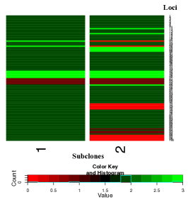
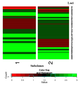
We assess the proposed model via simulation. We generate hypothetical read counts for a set of $S=100$ loci in $T=4$ hypothetical samples. In the simulation truth, we assume two latent subclones ($C^{{\mbox{\tiny TRUE}}}=2$) as well as a background subclone ($c=0$) with all SNVs bearing variant sequences with two copies. We use $Q=3$. The simulation truth $\bm{L}^{\mbox{\tiny TRUE}}$ is shown in Figure 3(a) where green color (light grey) in the panels indicates a copy gain ($\ell_{sc}=3$) and red color (dark grey) indicates two copy loss ($\ell_{sc}=0$). Panel (b) shows the simulation truth $\bm{Z}^{\mbox{\tiny TRUE}}$. Similar to $\bm{L}^{\mbox{\tiny TRUE}}$, green color indicates three copies with SNV and red color indicates zero copies with SNV. We generate $\phi^{\mbox{\tiny TRUE}}_{t}\stackrel{{\scriptstyle iid}}{{\sim}}\mbox{Gamma}(600,3)$, $t=1,\ldots,4$ and then generate $\bm{w}^{\mbox{\tiny TRUE}}\stackrel{{\scriptstyle iid}}{{\sim}}\mbox{Dir}(0.4,30.0,10.0)$. The weights $\bm{w}^{\mbox{\tiny TRUE}}$ are shown in Figure 3(c). Similar to the other heatmaps, green color (light grey) in panel (c) represents high abundance of a subclone in a sample and red color (dark grey) shows low abundance. On average, subclone 1 takes $w_{tc}$ close to 0.75 for all the samples, with little heterogeneity across samples. Using the assumed $\bm{L}^{\mbox{\tiny TRUE}}$, $\bm{Z}^{\mbox{\tiny TRUE}}$ and $\bm{w}^{\mbox{\tiny TRUE}}$ and letting $p_{0}^{\mbox{\tiny TRUE}}=0.05$, we generate $N_{st}\sim\mbox{Poi}(\phi_{t}^{\mbox{\tiny TRUE}}M_{st}^{\mbox{\tiny TRUE}}/2)$ and $n_{st}\sim\mbox{Bin}(N_{st},p^{\mbox{\tiny TRUE}}_{st})$.

(a) $\bm{L}^{\mbox{\tiny TRUE}}$	(b) $\bm{Z}^{\mbox{\tiny TRUE}}$	(c) $\bm{w}^{\mbox{\tiny TRUE}}$

Figure 3: Simulation 1: simulation truth.

To fit the proposed model, we fix the hyperparameters as $r=0.2$, $\alpha=2$, $\gamma_{q}=0.5$ for $q=0,1,3(=Q)$, $d_{0}=0.5$, $d=1$, $a_{00}=0.3$ and $b_{00}=5$. For the prior on $\phi_{t}$, we let $b=3$ and specify $a$ by setting the median of the observed $N_{st}$ to be the prior mean. For each value of $C$, we initialized $\bm{Z}$ using the observed sample proportions and $\bm{L}$ using the initial $\bm{Z}$. We generated initial values for $\bm{\theta}_{tc}$ and $p_{0}$ by prior draws. We generated $b_{st}\stackrel{{\scriptstyle iid}}{{\sim}}\mbox{Be}(25,975)$ to construct the training set and ran the MCMC simulation over 16,000 iterations, discarding the first 6,000 iterations as initial burn-in.

(a) $p(C\mid\bm{n},\bm{N})$	(b) $\hat{M}_{st}-M^{\mbox{\tiny TRUE}}_{st}$	(c) $\hat{p}_{st}-p^{\mbox{\tiny TRUE}}_{st}$
(d) $\bm{L}^{\star}$	(e) $\bm{Z}^{\star}$	(f) $\bm{w}^{\star}$

Figure 4: Posterior inference for Simulation 1.

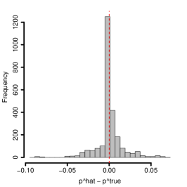
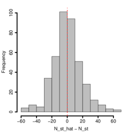
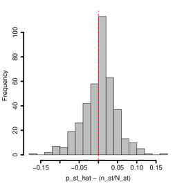
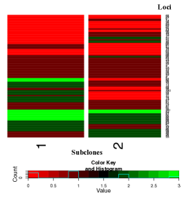
Figure 4(a) shows $p(C\mid\bm{n},\bm{N})$. The dashed vertical line marks the simulation truth $C^{{\mbox{\tiny TRUE}}}=2$. The posterior mode $C^{\star}=2$ recovers the truth. Panels (d) through (f) show the posterior point estimates, $\bm{L}^{\star}$, $\bm{Z}^{\star}$ and $\bm{w}^{\star}$. Compared to the simulation truth in Figure 3, the posterior estimate recovers subclone 1 with high accuracy, but $\bm{\ell}^{\star}_{c}$ for subclone $c=2$ shows some discrepancies with the simulation truth. This is due to small $w^{\mbox{\tiny TRUE}}_{tc}$, $c=2$, across all four samples (last column in Figure 3c). The discrepancy between $\bm{\ell}_{2}^{\star}$ and $\bm{\ell}_{2}^{\mbox{\tiny TRUE}}$ is related to the misspecification of $\bm{z}^{\star}_{c}$ under $c=2$. Conditional on $C^{\star}$, we computed $\hat{M}_{st}$ and $\hat{p}_{st}$ and compared to the true values. Figure 4(b) and (c) show a good fit under the model for a majority of loci and samples although the histograms include a small pocket of differences between the true values and their estimates on the right tail, also possibly due to the misspecification of $\bm{\ell}_{2}$ and $\bm{z}_{2}$. This simulation study illustrates that the proposed model reasonably recovers the simulation truth even with a small number of samples when the underlying structure is not complex.

(a) Cellular prevalences	(b) $p^{\mbox{\tiny TRUE}}_{st}$

Figure 5: Heatmaps of estimated cellular prevalences from PyClone (a) and $p_{st}^{\mbox{\tiny TRUE}}$ (b) for Simulation 1.

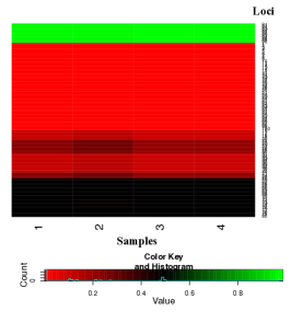
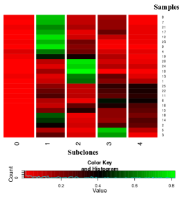
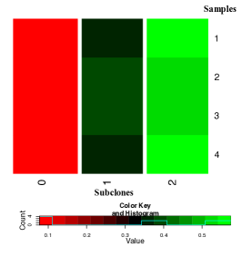
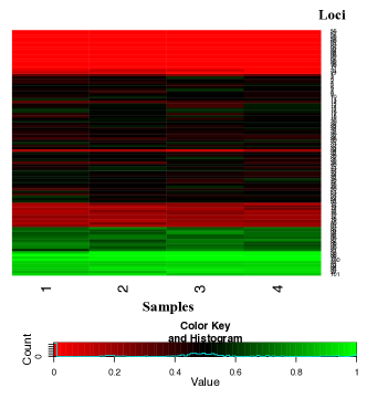
For comparison, we implemented PyClone (Roth et al., 2014) with the same simulated data. We let the normal copy number, the minor parental copy number and the major parental copy number be 2, 0 and 3, respectively, at each locus. PyClone considers copy number changes and estimates the variant allelic prevalence (fraction of clonal population having a mutation) at a locus in a sample. The interpretation of variant allelic prevalences, referred to as “cellular prevalences” in PyClone, is similar to that of $p_{st}$ in the proposed model. PyClone uses a Dirichlet process model to identify a (non-overlapping) clustering of the loci based on their cellular prevalences. Cellular prevalences over loci and samples may vary but the clustering of loci is shared by samples. Figure 5(a) shows posterior estimates of the cellular prevalences (by color and grey shade) and mutational clustering (by separations with white horizontal lines) under PyClone. Panel (b) of the figure shows a heatmap of $p_{st}^{\mbox{\tiny TRUE}}$. The loci (rows) of the two heatmaps are re-arranged in the same order for easy comparison. By comparing the two heatmaps, the cellular prevalence estimates under PyClone are close to $p_{st}^{\mbox{\tiny TRUE}}$ and lead to a reasonable estimate of a clustering of the loci. However, PyClone does not attempt to construct a description of subclones with genomic variants.

3.2 Simulation 2

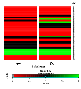
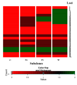
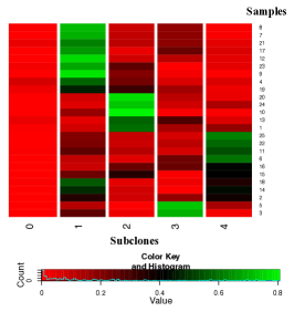
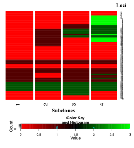
We carried out a second simulation study with a more complicated subclonal structure. We simulate read counts for a set of $S=100$ loci in $T=25$ hypothetical samples. In the simulation truth, we assume four latent subclones ($C^{{\mbox{\tiny TRUE}}}=4$) as well as a background subclone ($c=0$) with all SNVs bearing variant sequences with two copies. We use $Q=3$. The simulation truths, $\bm{L}^{\mbox{\tiny TRUE}}$ and $\bm{Z}^{\mbox{\tiny TRUE}}$ are shown in Figure 6(a) and (b), respectively. We generated $\phi^{\mbox{\tiny TRUE}}_{t}$ from $\mbox{Gamma}(600,3)$ for $t=1,\ldots,25$ and then generated $\bm{w}_{t}^{\mbox{\tiny TRUE}}$ as follows. We let $\bm{a}^{\mbox{\tiny TRUE}}=(13,4,2,1)$ and for each $t$ randomly permuted $\bm{a}^{\mbox{\tiny TRUE}}$. Let $\bm{a}_{\pi}^{\mbox{\tiny TRUE}}$ denote a random permutation of $\bm{a}^{\mbox{\tiny TRUE}}$. We generate $\bm{w}^{\mbox{\tiny TRUE}}\sim\mbox{Dir}(0.3,\bm{a}_{\pi}^{\mbox{\tiny TRUE}})$. That is, the first parameter of the Dirichlet prior for the $(C^{\mbox{\tiny TRUE}}+1)$-dimensional weight vector was $0.3$, and the remaining parameters were a permutation of $\bm{a}^{\mbox{\tiny TRUE}}$. The weights $\bm{w}^{\mbox{\tiny TRUE}}$ are shown in Figure 6(c). The samples in the rows are rearranged for better display. From Figure 6(c), each sample has all the four subclones with its own cellular fractions, resulting in large heterogeneity within a sample. In addition, the random permutation of $\bm{a}^{\mbox{\tiny TRUE}}$ induces heterogeneity among the samples. We observe that when the underlying subclonal structure is complicate and samples are heterogeneous, larger sample size is needed. In particular, $T=25$ which is a large number compared to the typical sample size in real datasets is assumed for this simulation study. Using the assumed $\bm{L}^{\mbox{\tiny TRUE}}$, $\bm{Z}^{\mbox{\tiny TRUE}}$ and $\bm{w}^{\mbox{\tiny TRUE}}$ and letting $p_{0}^{\mbox{\tiny TRUE}}=0.05$, we generate $N_{st}\sim\mbox{Poi}(\phi_{t}^{\mbox{\tiny TRUE}}M_{st}^{\mbox{\tiny TRUE}}/2)$ and $n_{st}\sim\mbox{Bin}(N_{st},p^{\mbox{\tiny TRUE}}_{st})$. We fit the proposed model as in the first simulation study.

(a) $\bm{L}^{\mbox{\tiny TRUE}}$	(b) $\bm{Z}^{\mbox{\tiny TRUE}}$	(c) $\bm{w}^{\mbox{\tiny TRUE}}$

Figure 6: Simulation 2: simulation truth.

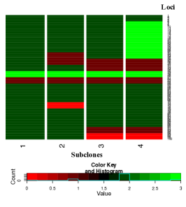
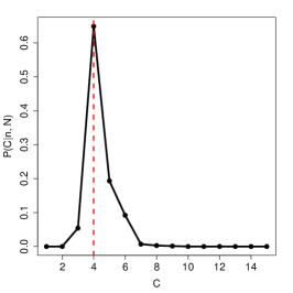
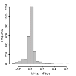
Figure 7(a) reports $p(C\mid\bm{n},\bm{N})$, again marking $C^{\mbox{\tiny TRUE}}$ with a dashed vertical line. The posterior mode $C^{\star}=4$ correctly recovers the truth. Panels (d) through (f) summarize the posterior point estimates, $\bm{L}^{\star}$, $\bm{Z}^{\star}$ and $\bm{w}^{\star}$. Posterior estimates accurately recover the simulation truth for subclones 1 and 2, for which the true proportions $w_{tc}^{\mbox{\tiny TRUE}}$ are large for many samples, as shown in Figure 6(c). On the other hand, the posterior estimate for subclones 3 and 4 shows discrepancies with the simulation truth. In particular, we observe that a group of loci that have $\ell^{\mbox{\tiny TRUE}}_{sc}=1$ in subclones 3 and 4 has $\ell^{\star}_{sc}=2$ for subclone 3 and $\ell^{\star}_{sc}=0$ for subclone 4. We suspect that this reflects the small weights $w^{\mbox{\tiny TRUE}}_{tc}$ for $c=3,4$ for almost all samples, as seen in the last two columns of Figure 6(c). Notice also the bias in the corresponding estimates, $z^{\star}_{sc}$ and $\bm{w}^{\star}_{tc}$, $c=3,4$. Despite ambiguity about the true latent structure, we find a good fit to the data. Conditional on $C^{\star}$, we computed $\hat{M}_{st}$ and $\hat{p}_{st}$ and compared to the true values. Figure 7(b) and (c) show the summaries that indicate a good fit.

(a) $p(C\mid\bm{n},\bm{N})$	(b) $\hat{M}_{st}-M^{\mbox{\tiny TRUE}}_{st}$	(c) $\hat{p}_{st}-p^{\mbox{\tiny TRUE}}_{st}$
(d) $\bm{L}^{\star}$	(e) $\bm{Z}^{\star}$	(f) $\bm{w}^{\star}$

Figure 7: Posterior inference for Simulation 2.

(a) Cellular prevalences	(b) $p^{\mbox{\tiny TRUE}}_{st}$

Figure 8: Heatmaps of estimated cellular prevalences from PyClone (a) and $p_{st}^{\mbox{\tiny TRUE}}$ (b) for Simulation 2.

For comparison, we again applied PyClone (Roth et al., 2014) to the same simulated data. We used a similar setting for PyClone as in the previous simulation. Figure 8(a) shows the estimated cellular prevalences. The reported clustering of loci (shown with by separations with white horizontal lines) is reasonable. Compare with the simulation truth $p_{st}^{\mbox{\tiny TRUE}}$ in panel (b). The loci (rows) of the two heatmaps are re-arranged in the same order for easy comparison. Again, PyClone does not attempt to reconstruct how subclones could explain the observed data and does not provide inference on the true subclonal structure in Figure 6.

4 Lung Cancer Data

We record whole-exome sequencing for four surgically dissected tumor samples taken from the same patient with lung cancer. We extracted genomic DNA from each tissue and constructed an exome library from these DNA using Agilent SureSelect capture probes. The exome library was then sequenced in paired-end fashion on an Illumina HiSeq 2000 platform. About 60 million reads - each 100 bases long - were obtained. Since the SureSelect exome was about 50 Mega bases, raw (pre-mapping) coverage was about 120 fold. We then mapped the reads to the human genome (version HG19) (Church et al., 2011) using BWA (Li and Durbin, 2009b) and called variants using GATK (McKenna et al., 2010a). Post-mapping, the mean coverage of the samples was between 60 and 70 fold.

A total of nearly 115,000 SNVs and small indels were called within the exome coordinates. We restricted our attention to SNVs that (i) make a difference to the protein translated from the gene, and (ii) that exhibit significant coverage in all samples with $n_{st}/N_{st}$ not being too close to 0 or 1; and (iii) we used expert judgment to some more loci. The described filter rules leave in the end $S=101$ SNVs for the four intra-tumor samples. Figure 9 shows the histograms of the total number of reads and the empirical read ratios, $N_{st}$ and $n_{st}/N_{st}$.

(a) Histogram of $N_{st}$	(b) Histogram of $n_{st}/N_{st}$

Figure 9: Histograms of the Lung Cancer Dataset.

(a) $p(C\mid\bm{n},\bm{N})$	(b) $\hat{N}_{st}-N_{st}$	(c) $\hat{p}_{st}-(n_{st}/N_{st})$
(d) $\bm{L}^{\star}$	(e) $\bm{Z}^{\star}$	(f) $\bm{w}^{\star}$

Figure 10: Posterior inference for the Lung Cancer Dataset.

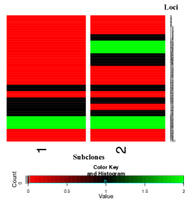
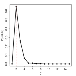
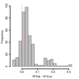
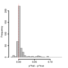
We used hyperparameters similar to those in the simulation studies. Figure 10 summarizes posterior inference under the proposed model. Panel (a) shows $C^{\star}=2$, i.e., two estimated subclones. Using posterior samples with $C=C^{\star}$, we computed $\hat{N}_{st}$ and $\hat{p}_{st}$ and compared them to the observed data. The differences are centered at 0, implying a good fit to the data. Conditional on $C^{\star}=2$, we found $\bm{L}^{\star}$, $\bm{Z}^{\star}$ and $\bm{w}^{\star}$. The loci in $\bm{L}^{\star}$ and $\bm{Z}^{\star}$ are re-arranged in the same order for better illustration. From Figure 9(a) we notice that many positions have large numbers of reads, over 200 reads. This is reflected in $\bm{L}^{\star}$ which estimates three copies at many positions. The estimated weights $\bm{w}^{\star}$ in Figure 10(f) show a great similarity across the four samples. This lack of heterogeneity across samples is not surprising. The four samples were dissected from close-by spatial locations in the tumor.

(a) Cellular prevalences	(b) $n_{st}/N_{st}$

Figure 11: Heatmaps of estimated cellular prevalences from PyClone (a) and $(n_{st}/N_{st})$ (b) for the Lung cancer dataset.

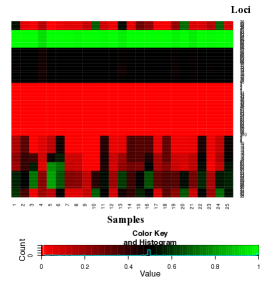
Again, for comparison implemented PyClone (Roth et al., 2014) for the lung cancer data. The posterior estimates of prevalence and the estimated clustering of the loci are shown in Figure 11(a). The clustering identified five clusters of the loci. The mean prevalences within a locus cluster are similar across samples, which is similar to $\bm{w}^{\star}$ in Figure 10(f). Panel (b) of Figure 11 is a heatmap of fractions of reads bearing mutation for each locus and sample. Again, PyClone provides a reasonable estimate of a loci clustering based on the empirical fractions, but does not provide an inference on subclonal populations.

5 Conclusions

The proposed approach infers subclonal DNA copy numbers, subclonal variant allele counts and cellular fractions in a biological sample. By jointly modeling CNV and SNV, we provide the desired description of TH based on DNA variations in both, sequence and structure. Such inference will significantly impact downstream treatment of individual tumors, ultimately allowing personalized prognosis. For example, tumor with large proportions of cells bearing somatic mutations on tumor suppressor genes should be treated differently from those that have no or a small proportion of such cells. In addition, metastatic or recurrent tumors may possess very different compositions of cellular genomes and should be treated differently. Inference on TH can be exploited for improved treatment strategies for relapsed cancer patients, and can spark significant improvement in cancer treatment in practice.

A number of extensions are possible for the present model. For example, sometimes additional sources of information on CNVs such as a SNP array may be available. We then extend the proposed model to incorporate this information into the modeling of $\bm{L}$. Another meaningful extension is to cluster patients on the basis of the imputed TH, that is, we link a random partition and a feature allocation model. This extension may help clinicians assign different treatment strategies, and be the basis of adaptive clinical trial designs.

Inference for TH is a critical gap in the current literature. The ability to precisely break down a tumor into a set of subclones with distinct genetics would provide the opportunity for breakthroughs in cancer treatment by facilitating individualized treatment of the tumor that exploits TH. It would open the door for cocktail type of combinational treatments, with each treatment targeting a specific tumor subclone based on its genetic characteristics. We believe that the proposed model may provide a integrated view on subclones to explain TH that remains a mystery to scientists so far.

References

- Bedard et al. (2013) Bedard, P. L., Hansen, A. R., Ratain, M. J., and Siu, L. L. (2013). Tumour heterogeneity in the clinic. Nature 501, 7467, 355–364.
- Biesecker and Spinner (2013) Biesecker, L. G. and Spinner, N. B. (2013). A genomic view of mosaicism and human disease. Nature Reviews Genetics 14, 5, 307–320.
- Broderick et al. (2013) Broderick, T., Jordan, M. I., Pitman, J., et al. (2013). Cluster and feature modeling from combinatorial stochastic processes. Statistical Science 28, 3, 289–312.
- Brooks et al. (2011) Brooks, S., Gelman, A., Jones, G., and Meng, X.-L. (2011). Handbook of Markov Chain Monte Carlo. CRC Press.
- Church et al. (2011) Church, D. M., Schneider, V. A., Graves, T., Auger, K., Cunningham, F., Bouk, N., Chen, H.-C., Agarwala, R., McLaren, W. M., Ritchie, G. R., et al. (2011). Modernizing reference genome assemblies. PLoS biology 9, 7, e1001091.
- De (2011) De, S. (2011). Somatic mosaicism in healthy human tissues. Trends in Genetics 27, 6, 217–223.
- Ding et al. (2012) Ding, L., Ley, T. J., Larson, D. E., Miller, C. A., Koboldt, D. C., Welch, J. S., Ritchey, J. K., Young, M. A., Lamprecht, T., McLellan, M. D., et al. (2012). Clonal evolution in relapsed acute myeloid leukaemia revealed by whole-genome sequencing. Nature 481, 7382, 506–510.
- Frank and Nowak (2003) Frank, S. A. and Nowak, M. A. (2003). Cell biology: Developmental predisposition to cancer. Nature 422, 6931, 494–494.
- Frank and Nowak (2004) Frank, S. A. and Nowak, M. A. (2004). Problems of somatic mutation and cancer. Bioessays 26, 3, 291–299.
- Greaves and Maley (2012) Greaves, M. and Maley, C. C. (2012). Clonal evolution in cancer. Nature 481, 7381, 306–313.
- Jiao et al. (2014) Jiao, W., Vembu, S., Deshwar, A., Stein, L., and Morris, Q. (2014). Inferring clonal evolution of tumors from single nucleotide somatic mutations. BMC Bioinformatics 15, 1, 35.
- Kim et al. (2012) Kim, Y., James, L., and Weissbach, R. (2012). Bayesian analysis of multistate event history data: beta-dirichlet process prior. Biometrika 99, 1, 127–140.
- Klambauer et al. (2012) Klambauer, G., Schwarzbauer, K., Mayr, A., Clevert, D.-A., Mitterecker, A., Bodenhofer, U., and Hochreiter, S. (2012). cn. mops: mixture of poissons for discovering copy number variations in next-generation sequencing data with a low false discovery rate. Nucleic Acids Research 40, 9, e69–e69.
- Lee et al. (2014) Lee, J., Müller, P., Gulukota, K., and Ji, Y. (2014). A bayesian feature allocation model for tumor heterogeneity.
- Li and Li (2014) Li, B. and Li, J. Z. (2014). A general framework for analyzing tumor subclonality using SNP array and DNA sequencing data. Genome Biology in press.
- Li and Durbin (2009a) Li, H. and Durbin, R. (2009a). Fast and accurate short read alignment with Burrows–Wheeler transform. Bioinformatics 25, 14, 1754–1760.
- Li and Durbin (2009b) Li, H. and Durbin, R. (2009b). Fast and accurate short read alignment with burrows–wheeler transform. Bioinformatics 25, 14, 1754–1760.
- Li et al. (2009) Li, H., Handsaker, B., Wysoker, A., Fennell, T., Ruan, J., Homer, N., Marth, G., Abecasis, G., Durbin, R., et al. (2009). The sequence alignment/map format and samtools. Bioinformatics 25, 16, 2078–2079.
- McKenna et al. (2010a) McKenna, A., Hanna, M., Banks, E., Sivachenko, A., Cibulskis, K., Kernytsky, A., Garimella, K., Altshuler, D., Gabriel, S., Daly, M., et al. (2010a). The genome analysis toolkit: a mapreduce framework for analyzing next-generation dna sequencing data. Genome research 20, 9, 1297–1303.
- McKenna et al. (2010b) McKenna, A., Hanna, M., Banks, E., Sivachenko, A., Cibulskis, K., Kernytsky, A., Garimella, K., Altshuler, D., Gabriel, S., Daly, M., et al. (2010b). The Genome Analysis Toolkit: a MapReduce framework for analyzing next-generation DNA sequencing data. Genome research 20, 9, 1297–1303.
- Miller et al. (2014) Miller, C. A., White, B. S., Dees, N. D., Griffith, M., Welch, J. S., Griffith, O. L., Vij, R., Tomasson, M. H., Graubert, T. A., Walter, M. J., et al. (2014). Sciclone: Inferring clonal architecture and tracking the spatial and temporal patterns of tumor evolution. PLoS computational biology 10, 8, e1003665.
- Navin et al. (2011) Navin, N., Kendall, J., Troge, J., Andrews, P., Rodgers, L., McIndoo, J., Cook, K., Stepansky, A., Levy, D., Esposito, D., et al. (2011). Tumour evolution inferred by single-cell sequencing. Nature 472, 7341, 90–94.
- Oesper et al. (2013) Oesper, L., Mahmoody, A., and Raphael, B. J. (2013). Theta: inferring intra-tumor heterogeneity from high-throughput dna sequencing data. Genome Biol 14, 7, R80.
- Roth et al. (2014) Roth, A., Khattra, J., Yap, D., Wan, A., Laks, E., Biele, J., Ha, G., Aparicio, S., Bouchard-Côté, A., and Shah, S. P. (2014). Pyclone: statistical inference of clonal population structure in cancer. Nature methods .
- Russnes et al. (2011) Russnes, H. G., Navin, N., Hicks, J., and Borresen-Dale, A.-L. (2011). Insight into the heterogeneity of breast cancer through next-generation sequencing. The Journal of Clinical Investigation 121, 10, 3810–3818.
- Sengupta (2013) Sengupta, S. (2013). Two models involving bayesian nonparametric techniques (ph.d thesis).
- Sengupta et al. (2015) Sengupta, S., Guluokta, K., Lee, J., Müller, P., and Ji, Y. (2015). Bayclone: Bayesian nonparametric inference of tumor subclones using ngs data. In Proceedings of The Pacific Symposium on Biocomputing (PSB) 2015, in press.
- Strino et al. (2013) Strino, F., Parisi, F., Micsinai, M., and Kluger, Y. (2013). Trap: a tree approach for fingerprinting subclonal tumor composition. Nucleic Acids Research 41, 17, e165.
- Zare et al. (2014) Zare, H., Wang, J., Hu, A., Weber, K., Smith, J., Nickerson, D., Song, C., Witten, D., Blau, C. A., and Noble, W. S. (2014). Inferring clonal composition from multiple sections of a breast cancer. PLoS computational biology 10, 7, e1003703.