Fragmentation of Random Trees

Abstract

We study fragmentation of a random recursive tree into a forest by repeated removal of nodes. The initial tree consists of $N$ nodes and it is generated by sequential addition of nodes with each new node attaching to a randomly-selected existing node. As nodes are removed from the tree, one at a time, the tree dissolves into an ensemble of separate trees, namely, a forest. We study statistical properties of trees and nodes in this heterogeneous forest, and find that the fraction of remaining nodes $m$ characterizes the system in the limit $N\to\infty$. We obtain analytically the size density $\phi_{s}$ of trees of size $s$. The size density has power-law tail $\phi_{s}\sim s^{-\alpha}$ with exponent $\alpha=1+\tfrac{1}{m}$. Therefore, the tail becomes steeper as further nodes are removed, and the fragmentation process is unusual in that exponent $\alpha$ increases continuously with time. We also extend our analysis to the case where nodes are added as well as removed, and obtain the asymptotic size density for growing trees.

I Introduction

Random trees hmm ; md underlie a variety of physical processes including collisions vv ; bkm , fragmentation km , and fractal aggregation ym . These random structures are found in data storage and retrieval in computer science dek ; jmr ; bp ; ld and they provide a framework for studies in biological evolution teh ; msw ; dekm ; mp .

Previous studies of random trees typically deal with random structures generated by sequential addition of nodes hmm ; md . The same holds for widely-used models of network formation which generally describe strictly growing networks dm ; ba ; dms ; krl ; mejn . Yet, in many applications including social networks deb ; ptn ; cpchbls , evolutionary trees msw ; dekm , and technological networks, nodes may disappear so the network can increase or decrease in size.

A number of recent studies of trees formed by addition and removal of nodes focus on the connectivity of individual nodes and in particular, the degree distribution mgn ; fc ; bk ; js ; bmrs ; sdh . Node removal can cause fragmentation into separate connected components (see Figure 1). Yet, theoretical tools for analyzing connected components in random structures undergoing fragmentation are limited mejn ; cpchbls and statistical properties of groups of connected nodes in such processes remain largely an open question.

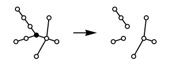
Figure 1: The fragmentation process. Removal of the indicated node (filled circle) fragments a tree of size $N=10$ (left) into three separate trees with sizes $s=4$, $s=3$, and $s=2$ (right). Each fragment correspond to a branch of that node.

Here, we analyze connected components of a random recursive tree undergoing fragmentation caused by removal of nodes. The original tree is formed by sequential addition of nodes: in each elementary step one node is added and it is attached to an existing node that is selected at random. This process is repeated until a tree with $N$ nodes forms. As nodes are removed from the tree, it fragments into multiple connected components, each having a tree structure. The resulting “forest” consists of multiple trees (see Figure 2). Our main goal is to find the size distribution of connected components in this heterogeneous forest.

As a preliminary step, we establish the fragment-size distribution when a single node is removed. This quantity plays the role of a “kernel” for the fragmentation process that ensues as nodes are repeatedly removed from the system. We use a dynamical formulation where the number of nodes plays the role of time, and use rate equations to describe how the fragment-size distribution evolves. We find the fragment-size distribution analytically as a function of the fraction of remaining nodes $m$ in the limit $N\to\infty$. The density $\phi_{s}$ of fragments of size $s$ has the algebraic tail

$$\phi_{s}\sim s^{-\alpha}\qquad\text{with}\qquad\alpha=1+\frac{1}{m}.$$ (1)

When an infinitesimal fraction of nodes are removed, the tail is the broadest, $\phi_{s}\sim s^{-2}$, but throughout the fragmentation process, the distribution becomes gradually narrower. The exponent $\alpha$ increases monotonically with time and it ultimately diverges when a finite number of nodes remain.

We also consider growing forests formed by simultaneous addition and removal of nodes. In this case, the size distribution is narrower as it has an exponential tail.

The rest of this article is organized as follows. We first describe the tree fragmentation process and define the fragment size density (Section II). In Section III, we consider fragmentation by removal of a single node and derive the fragment-size density as a function of size $N$. This quantity allows us to write recursion relations for the evolution of the size density throughout the fragmentation process. We obtain a scaling solution where the fraction of remaining nodes $m$ plays the role of a scaling variable (Section IV). In Section V, we consider the situation where nodes are added and removed at constant rates, and obtain the leading asymptotic behavior for very large fragments. We conclude with a summary and a discussion in Sec. VI. The Appendix details a few technical derivations.

II The fragmentation process

We study fragmentation of a random tree through sequential removal of nodes. The starting point is a random recursive tree hmm ; md . This tree is generated by sequential addition of nodes with each new node attached to a randomly-selected existing node. Starting with one isolated node, this process repeats until the tree reaches initial size $N$. The tree has $N-1$ links and hence, it has no loops.

In each time step, one node is selected at random and it is removed from the system together with all of the links connected to it. Hence, the total number of nodes $M$ at time $t$ is simply

$$M(t)=N-t.$$ (2)

At time $t=0$ there are $N$ nodes, and the process ends at time $t=N-1$ with a single remaining node.

As nodes are removed from the system, the tree fragments into multiple connected components. Figure 1 depicts removal of the very first node and Figure 2 shows the resulting forest after a finite fraction nodes have been removed. Removal of nodes dissolves the tree into an ensemble of connected components, each having a tree structure.

The evolving forest is a collection of distinct trees and our primary goal is to characterize the sizes of trees in this heterogeneous forest. Let $F_{s,N}(t)$ be the average number of trees of size $s$ at time $t$ in a system of (initial) size $N$. This quantity corresponds to an average over infinitely many independent realizations of the tree generation process and over infinitely many independent realizations of the node removal process. The initial condition is a single tree of size $s=N$, $F_{s,N}(0)=\delta_{s,N}$, and the final state is a single node, $F_{s,N}(N-1)=\delta_{s,1}$.

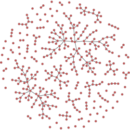
Figure 2: The random forest. Shown is a representative example where fraction $m=3/4$ of the initial $N=500$ nodes remain.

The total number of trees is deterministic only at the initial and the final state, but generally, this quantity fluctuates from realization to realization. In contrast, the total number of nodes (2) is a deterministic quantity. The number of nodes normalizes the fragment-size density

$$\sum_{s}s\,F_{s,N}(t)=N-t.$$ (3)

Our main goal is to find the fragment-size density as a function of time in the limit $N\to\infty$.

III The branch-size density

As a preliminary step, we study $F_{s,N}(1)$, the fragment-size density after a single node has been removed. We define a branch as the subtree attached to a node through one of its links. Figure 1 shows that removal of a node with three links and hence three branches, leads to three fragments. Therefore, there is a one-to-one correspondence between the branches of a node and the fragments generated when that node is removed. Of course, the number of branches equals the node degree.

Let $P_{s,N}$ be the average number of branches containing $s$ nodes of a randomly selected node in a random recursive tree of size $N$. This quantity is equivalent to the fragment-size density at time $t=1$, that is $P_{s,N}\equiv F_{s,N}(1)$.

The zeroth moment of the branch-size density gives the average number of branches per node and the first moment gives the total number of nodes minus one,

$$\sum_{s}P_{s,N}=\frac{2(N-1)}{N},\qquad\sum_{s}s\,P_{s,N}=N-1.$$ (4)

A tree with $N$ nodes has $N-1$ links and every link connects two branches. Hence, the total number of branches is $2(N-1)$, and the average number of branches per node is simply $2(N-1)/N$. The second identity follows from (3).

The density $P_{s,N}$ satisfies the recursion equation

$$P_{s,N+1} = \frac{N}{N+1}\left(\frac{s-1}{N}P_{s-1,N}+\frac{N-s}{N}P_{s,N}\right)$$ (5)

$$+ \frac{1}{N+1}\left(\delta_{s,1}+\delta_{s,N}\right).$$

This recursion is subject to the “initial condition” $P_{s,1}=0$. The first two terms account for contributions from existing branches while the last two terms represent branches created by the newly added node; hence the respective weights $\tfrac{1}{N+1}$ and $\tfrac{N}{N+1}$. When a new node attaches to a branch of size $s$, the branch size grows by one, that is, $s\to s+1$. A branch of size $s$ consequently expands with probability $\tfrac{s}{N}$; otherwise the branch maintains its size with probability $\tfrac{N-s}{N}$. The last two terms reflect that a new link generates two new branches, one of size $s=1$ and one of size $s=N$. By summing (5), it is possible to check that the recursion is compatible with the sum rules (4).

Using the recursion relations (5) we can find the branch-size density for small trees. Starting with $P_{s,1}=0$ we arrive at

$$P_{s,N}\!=\!\begin{cases}\delta_{s,1}&$N=2$,\\ \tfrac{2}{3}\delta_{s,1}+\tfrac{2}{3}\delta_{s,2}&$N=3$,\\ \tfrac{7}{12}\delta_{s,1}+\tfrac{1}{3}\delta_{s,2}+\tfrac{7}{12}\delta_{s,3}&$N=4$,\\ \tfrac{11}{20}\delta_{s,1}+\tfrac{1}{4}\delta_{s,2}+\tfrac{1}{4}\delta_{s,3}+\tfrac{11}{20}\delta_{s,4}&$N=5$.\end{cases}$$ (6)

It is also possible to check these expressions by enumerating all possible tree morphologies for $2\leq N\leq 5$ and removing a randomly-selected node. Also, the densities listed in (6) satisfy the sum rules (4).

The expressions (6) suggest that the fragment-size density is symmetric, $P_{s,N}=P_{N-s,N}$. This symmetry reflects that the recursion relation (5) is invariant under the transformation $s\to N-s$. Moreover, equation (6) suggest the general expression

$$P_{s,N}=\frac{1}{s(s+1)}+\frac{1}{(N-s)(N+1-s)},$$ (7)

for $1\leq s\leq N-1$. The small-$s$ expressions adhere to this general form for all $2\leq N\leq 5$ and all $1\leq s\leq N-1$. For example, $P_{1,5}=\tfrac{1}{1\cdot 2}+\tfrac{1}{4\cdot 5}$ and $P_{2,5}=\tfrac{1}{2\cdot 3}+\tfrac{1}{3\cdot 4}$. Furthermore, equation (7) can be justified by induction. When $N=2$, we have $P_{1,2}=1$ and the expression (7) satisfies the recursion equation (5) for all $1\leq s\leq N-1$. We also note that the first term $\tfrac{1}{s(s+1)}$ in (7) which does not depend on tree size $N$ coincides with the distribution of in-component size for a random tree bk .

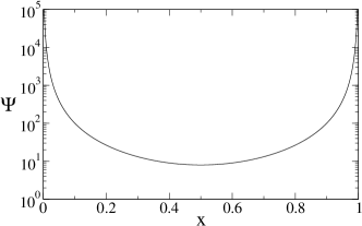
Figure 3: The scaling function $\Psi$ versus the scaling variable $x$.

For very large trees, $N\gg 1$, the density (7) adheres to the scaling form $P_{s,N}\simeq(1/N^{2})\Psi\left(s/N\right)$. In terms of the normalized branch size $x=s/N$, the scaling function is (see Figure 3)

$$\Psi(x)=\frac{1}{x^{2}}+\frac{1}{(1-x)^{2}},$$ (8)

for $0<x<1$ and it has the symmetry $\Psi(x)=\Psi(1-x)$. We note that the fragment-size density has a power-law tail $F_{s,N}(1)\sim s^{-2}$ for $s\ll N$ in the limit $N\to\infty$.

IV The fragment-size density

We now consider the distribution of fragment size after multiple nodes have been removed from the system. Importantly, every fragment is itself a random recursive tree. Indeed, every fragment is a piece of the original tree, that is, a subset of connected nodes. Further, this subset expands by same growth mechanism that governs the entire tree. If a new node is attached to this subset, then every one of the nodes is equally likely to receive this new connection.

This key observation allows us to treat the problem analytically. Since fragments are equivalent to the initial tree, the outcome of the very first fragmentation event characterizes all subsequent fragmentation events. Consequently, the tree fragmentation process reduces to an ordinary fragmentation process cr ; zm ; es . Throughout this process, a random tree of size $l$ generates a fragment of size $1\leq s\leq l-1$ with probability $P_{s,l}$ rmz ; dlb . Hence, the tree morphology is entirely encapsulated by the fragmentation kernel $P_{s,l}$ given in (7).

The fragment-size density evolves according to the linear recursion equation

$$F_{s}(t+1)=F_{s}(t)-sf_{s}(t)+\sum_{l>s}l\,f_{l}(t)\,P_{s,l}.$$ (9)

Here, we introduce the rescaled density $f_{s}(t)=F_{s}(t)/\sum_{s}s\,F_{s}(t)$, with the normalization $\sum_{s}s\,f_{s}=1$; this normalization reflects that the probability a randomly-selected node resides in a tree of size $s$ equals $s\,f_{s}$. Henceforth, the dependence on system size is made implicit, $F_{s}(t)\equiv F_{s,N}(t)$. The recursion equation (9) describes the tree fragmentation process. The loss term equals fragment size because the probability the removed node belongs to a tree is proportional to tree size. The gain term reflects the fragmentation process: trees fragment with probability proportional to their size and hence the term $l\,f_{l}$, while the second quantity $P_{s,l}$ is simply the fragmentation kernel. We can verify, using the second identity in (4), that the total number of nodes $M=\sum_{s}s\,F_{s}$ decreases by one in each fragmentation event in agreement with (2).

Starting with the initial condition $F_{s}(0)=\delta_{s,N}$, we iterate the recursion equation (9) once and by construction, recover the fragmentation kernel $F_{s}(1)=P_{s,N}$. We now substitute the expressions (6) for small $N$ and iterate the recursion (9) a second time to obtain the fragment-size density once two nodes are removed,

$$F_{s}(2)=\begin{cases}\delta_{s,1}&$N=3$\\ \delta_{s,1}+\tfrac{1}{2}\delta_{s,2}&$N=4$\\ \tfrac{59}{60}\delta_{s,1}+\tfrac{13}{30}\delta_{s,2}+\tfrac{23}{60}\delta_{s,3}&$N=5$.\\ \end{cases}$$ (10)

These expressions can be manually verified by exact enumeration. Removal of a second node breaks the symmetry in (7) because small fragments become more probable at the expense of large ones.

Our main interest is the behavior in the limit $N\to\infty$. In this limit, we can treat time as a continuous variable and convert the difference equation (9) into the differential equation

$$\frac{dF_{s}}{dt}=-sf_{s}+\sum_{l>s}l\,f_{l}\,P_{s,l}.$$ (11)

The total number of nodes $M=\sum_{s}F_{s}$ and the total number of trees in the forest $T=\sum_{s}F_{s}$ obey the differential equations $dM/dt=-1$ and $dT/dt=1-2T/M$, respectively. These evolution equations are obtained by summing the rate equations (9) and employing the first two moments of the fragmentation kernel (4). Using the initial conditions $M(0)=N$ and $T(0)=1$ we obtain the leading behavior in the limit $N\to\infty$

$$M=N\,m,\qquad\text{and}\qquad T=N\,m\,(1-m).$$ (12)

Here, we introduce the fraction of remaining nodes $m=(N-t)/N$. As expected, the number of nodes and trees are both proportional to system size. As a result, the average tree size $\langle s\rangle$ is given by $\langle s\rangle=(1-m)^{-1}$.

The quantities $M$ and $T$ suggest that the fraction of remaining nodes $m$ characterizes the state of the system in the limit $N\to\infty$. Results of numerical integration of the recursion equation (9) confirm that the fragment-size density depends only on the fraction of remaining nodes in this limit (see figure 4). Hence, we seek a scaling solution for the fragment-size density. Formally, the scaling solution $\phi_{s}$ is defined by

$$\phi_{s}(m)=\lim_{\begin{subarray}{c}N\to\infty\\ t\to\infty\end{subarray}}\frac{F_{s,N}\left(t\right)}{\sum_{s}s\,F_{s,N}(t)}$$ (13)

with $m=(N-t)/N$ kept fixed. The fragment-size density which in principle depends on two variables, system size $N$ and time $t$, becomes a function of a single scaling variable, the fraction of remaining nodes $m$ in the large-size limit. The quantity $s\,\phi_{s}$ is the probability that a randomly selected node is part of a tree of size $s$, and accordingly $\sum_{s}s\,\phi_{s}=1$.

We now substitute $F_{s}=M\,\phi_{s}$ into the rate equation (11) and introduce the time variable $\tau=\int_{0}^{t}dt^{\prime}[1/M(t^{\prime})]$ such that $d\tau/dt=1/M$. This time variable is related to the fraction of remaining nodes $m=e^{-\tau}$. With these transformations, the normalized density $\phi_{s}\equiv\phi_{s}(\tau)$ obeys the rate equation

$$\frac{d\phi_{s}}{d\tau}\!=\!(1\!-\!s)\phi_{s}\!+\!\sum_{l>s}\!\left[\frac{l\,\phi_{l}}{s(s+1)}\!+\!\frac{l\,\phi_{l}}{(l-s)(l+1-s)}\right]\!.$$ (14)

Here, we used the explicit form of $P_{s,l}$.

Results of the numerical integration of (9) suggest that the tail of the size density is algebraic (see Figure 4). Furthermore, in Appendix A we show that asymptotic analysis of the rate equation (14) yields the power-law decay (1). In a number of random structures including networks generated by preferential attachment, power-law tails correspond to ratios of Gamma functions krb . In these contexts, a ratio of Gamma functions is the discrete analog of an algebraic function of a continuous variable. As we show below, such behavior applies to our fragmentation process.

We postulate that the size distribution is a ratio of Gamma functions

$$\phi_{s}=(\alpha-2)\frac{\Gamma(s)\Gamma(\alpha)}{\Gamma(s+\alpha)},$$ (15)

for all $s\geq 1$ with the to-be-determined parameter $\alpha$. The prefactor is set by the normalization $\sum_{s}s\,\phi_{s}=1$. In appendix B, we show that $\phi_{s}$ in (15) satisfies the “evolution” equation

$$(\alpha\!-\!1)\frac{d\phi_{s}}{d\alpha}\!=\!(1\!-\!s)\phi_{s}\!+\!\sum_{l>s}\!\left[\!\frac{l\,\phi_{l}}{s(s\!+\!1)}\!+\!\frac{l\,\phi_{l}}{(l\!-\!s)(l\!+\!1\!-\!s)}\!\right]$$ (16)

for all $s\geq 1$. This equation describes how $\phi_{s}(\alpha)$ changes as function of $\alpha$. Since the right-hand sides of (14) and (16) are identical, the original rate equation (14) is satisfied if $d\phi_{s}/d\tau=(\alpha-1)d\phi_{s}/d\alpha$. Thus, we deduce that (15) is a solution of the evolution equation (14) when the parameter $\alpha$ evolves according to

$$\frac{d\alpha}{d\tau}=\alpha-1.$$ (17)

Together with the initial condition $\alpha(0)=2$ that follows from (7), we obtain $\alpha=1+e^{\tau}$ and find the parameter $\alpha$ as a function of remaining nodes,

$$\alpha=1+\frac{1}{m}.$$ (18)

Equations (15) and (18) constitute the exact solution for the scaling function defined in (13). From this solution, we can recover the average tree size, $\langle s\rangle=1/(1-m)$. The fraction of trees can also be obtained explicitly for small tree sizes

$$\phi_{1}=\frac{1-m}{1+m},\qquad\phi_{2}=\frac{1-m}{1+m}\frac{m}{1+2m}.$$ (19)

The results (15) and (18) establish our main result announced in (1). Using the asymptotic behavior $\Gamma(x)/\Gamma(x+a)\to x^{-a}$ as $x\to\infty$ we deduce $\phi_{s}\simeq C\,s^{-\alpha}$ with prefactor $C=(\alpha-2)\Gamma(\alpha)$ and exponent $\alpha$ given in (18). This prefactor vanishes in the limit $\alpha\to 2$ because the number of trees vanishes according to (12).

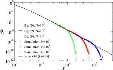
Figure 4: The size density $f_{s}\equiv F_{s}/M$ versus $s$ for the case $m=1/2$. Shown are: (i) results of numerical iteration of the recursion equation (9) for $N=10^{3}$, $N=10^{4}$, and $N=10^{5}$ (color lines); (ii) corresponding results of Monte Carlo simulations (color circles); and (iii) The limiting distribution (15) [black line]. Simulation results represent an average over $4.5\times 10^{4}$, $5\times 10^{2}$, and $10^{2}$ independent realizations with $N=10^{3}$, $N=10^{4}$, and $N=10^{5}$, respectively.

The exponent $\alpha$ increases monotonically throughout the fragmentation process. This behavior shows that the tail of the size density becomes gradually steeper as more nodes are removed. The size density (1) also has the unusual property that the exponent governing the tail is time dependent, $\alpha=1+\tfrac{N}{N-t}$. Power-law tails with fixed exponents have been observed in models of fragmentation bk1 ; kbg ; kb ; pd . Hence, the tree fragmentation process which has an unusual nonmonotonic fragmentation kernel (7) also has the unusual property that the power-law exponent varies continuously with time. In many fragmentation processes, the size distribution becomes universal, namely, it does not evolve with time, once the fragment size is scaled by the typical fragment size krb . Fragmentation of random trees does not follow this generic pattern as manifest from the fact that the exponent (18) is not fixed.

The power-law tail (1) shows that the forest created by the node removal process is heterogeneous and includes trees of a variety of sizes (Figure 2). When the size of the initial tree $N$ is large but finite, the solution (15) and its power-law tail (1) hold only for sizes $s\ll s_{\rm max}$. The size distribution is sharply suppressed beyond this maximal scale which represents the size of the largest tree in the forest. The cutoff scale $s_{\rm max}$ can be obtained by the extreme statistics criterion $1\sim N\sum_{s_{\rm max}}f_{s}$. From this heuristic argument, the cutoff grows algebraically with system size

$$s_{\rm max}\sim N^{m}.$$ (20)

Hence, as more nodes are removed, the range of validity of (15) and (1) shrinks. For example, when $m=1/2$ then $s_{\rm max}\sim\sqrt{N}$ and as shown in figure 4, the rate of convergence toward the $N\to\infty$ limiting behavior slows down with increasing $N$. In particular, astronomically large trees are needed to realize the power-law behavior (1) in the limit $m\to 0$.

We verified the theoretical predictions using direct integration of the recursion equation (9) and using Monte Carlo simulations of the tree fragmentation process (figure 4). The Monte Carlo simulation results agree with numerical solution of the recursion equation (9) for finite $N$. This agreement supports the assertion that fragments remain statistically equivalent to random recursive trees throughout the fragmentation process. Also, the numerical results agree with the scaling behavior (13). Finally, we confirmed the scaling function (15) for the case $m=1/2$ for which $\phi_{s}=2[s(s+1)(s+2)]^{-1}$.

The Monte Carlo simulations were performed by mimicking the tree creation and fragmentation processes. To generate the initial configuration, a random recursive tree of size $N$ was constructed. The tree is formed by sequential addition of nodes. The attachment probability is uniform such that every existing node is equally likely to receive a new link. Then, nodes are removed, one at a time, until $M$ nodes remain. The simulation results presented in this paper represent an average over multiple independent realizations of the tree creation and node removal processes.

For completeness, we briefly mention the degree distribution. We consider links to be directed and restrict our attention to the in-degree distribution. Let $A_{k}(m)$ be the average number of nodes with $k$ incoming links once $m$ nodes have been removed. It is well known that for the random recursive tree, the degree distribution is exponential, $A_{k}(0)=N\,2^{-k-1}$ krb . Since the fragments remain equivalent to a random recursive tree, we expect the degree distribution to remain exponential. By generalizing similar calculations in refs. mejn ; mgn ; krb , it is simple to obtain the in-degree distribution

$$A_{k}=N\,\alpha^{-k-1}.$$ (21)

The in-degree distribution remains exponential throughout the fragmentation process and the exponent $\alpha$ governs the exponential decay of the in-degree distribution.

V Addition and Removal of Nodes

Several recent studies have addressed the situation where nodes can be added or removed mgn ; fc ; bk ; js ; bmrs ; sdh . In this Section, we consider the case where nodes are added at constant rate $r$ and removed (as above) with unit rate. Both processes are completely random: a newly added node links to a randomly selected node, and nodes are selected at random for removal. Initially, the system consists of a single node $M(0)=1$. The number of nodes obeys the rate equation $dM/dt=r-1$ and hence, it grows steadily with time

$$M(t)=1+(r-1)t.$$ (22)

We restrict our attention to the growing case, $r>1$. The total number of trees $T$ is not affected by the addition process, so it evolves according to $dT/dt=1-2T/M$ as above. Solving this rate equation subject to the initial condition $T(0)=1$, we express the number of trees as a function of the number of nodes

$$T(M)=\frac{1}{r+1}\,M+\frac{r}{r+1}M^{-2/(r-1)}.$$ (23)

In the long-time limit, the average tree-size does not depend on time, $\langle s\rangle\to r+1$ as $t\to\infty$. The second term in (23) is negligible in this limit, and we thus conclude that statistical properties of the forest are characterized by the parameter $r$ alone.

It is straightforward to generalize the evolution equation (11) for $F_{s}(t)$ the average number of trees of size $s$ at time $t$,

$$\frac{dF_{s}}{dt}=r\left[(s\!-\!1)f_{s-1}\!-\!sf_{s}\right]\!-\!sf_{s}(t)\!+\!\sum_{l>s}l\,f_{l}(t)\,P_{s,l}.$$ (24)

The initial condition is $F_{s}(0)=\delta_{s,1}$. The first two terms characterize changes due to node addition and simply reflect that the probability a tree expands by addition of a new node is proportional to its size. In writing (24) we assume that fragments are statistically equivalent to a random recursive tree. By summing this rate equation, we can verify $dM/dt=r-1$.

Since the average size approaches a constant, we expect that the normalized size density $F_{s}/M$ approaches a steady state. Hence, we define the limiting size-density $\phi_{s}=\lim_{t\to\infty}F_{s}(t)/\sum_{s}s\,F_{s}(t)$. From the evolution equation (24) we deduce that this limiting distribution obeys

$$0 = r\,[(s-1)\phi_{s-1}-(s+1)\phi_{s}]$$

$$- (s-1)\,\phi_{s}+\sum_{l>s}\left[\frac{l\,\phi_{l}}{s(s+1)}+\frac{l\,\phi_{l}}{(l-s)(l+1-s)}\right].$$

We restrict our attention to very large trees. The simulation results suggest that the tail of the size density is exponential, although there is an algebraic correction,

$$\phi_{s}\sim s^{-\beta}\,\gamma^{s}\,,$$ (26)

for $s\gg 1$. For such a distribution, the first sum in (V) is negligible compared with the second sum, and the leading behavior of the second sum is (see Appendix C)

$$\sum_{l>s}\frac{l\,\phi_{l}}{(l-s)(l+1-s)}\simeq(c_{1}\,s+c_{2})\,\phi_{s},$$ (27)

in the limit $s\to\infty$. The two constants are $c_{1}=1+\big{(}\gamma^{-1}-1\big{)}\ln(1-\gamma)$ and $c_{2}=(\beta-1)\left[1+\gamma^{-1}\ln(1-\gamma)\right]$. By substituting (27) into (V), we obtain the recursion relation

$$\left(r+1-c_{1}+\frac{r-1-c_{2}}{s}\right)\phi_{s}\simeq r\left(1-\frac{1}{s}\right)\phi_{s-1}$$ (28)

that applies for very large sizes, $s\to\infty$. By comparing the two dominant terms, we confirm the leading exponential behavior $\phi_{s}\sim\gamma^{s}$ with $(r+1-c_{1})\gamma=r$. This gives $\gamma=1-e^{-r}$. Next, we substitute (26) into (28) and compare the magnitudes of the leading corrections $\propto s^{-1}$ to find $\gamma(r-1-c_{2})=r(\beta-1)$. Hence, $\beta=r$, and the tail of the size density decays according to

$$\phi_{s}\sim s^{-r}\left(1-e^{-r}\right)^{s}.$$ (29)

As the addition rate $r$ grows, the power-law becomes steeper but the exponential becomes shallower. Consequently, the two terms become comparable over a growing range with the cross-over scale $s_{*}\sim e^{r}$. When $s\ll s_{*}$, the powerlaw decay is dominant and only when $s\gg s_{*}$ does the distribution decay exponentially. We also note that in the presence of addition, very large trees become less probable and the forest becomes less heterogeneous.

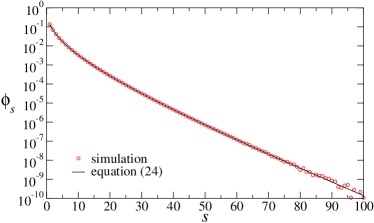
Figure 5: The size distribution $\phi_{s}$ versus $s$ for the case $r=2$. Shown are results of numerical integration of equation (24). Also shown are results of Monte Carlo simulations for $t=10^{7}$, averaged over $8.5\times 10^{3}$ independent runs.

We numerically simulated the node addition and removal process. In each simulation step, with probability $\tfrac{r}{r+1}$ a new node is added and with probability $\tfrac{1}{r+1}$ one node is deleted. Time is augmented as follows, $t\to t+\tfrac{1}{1+r}$ after each step. When a single node remains, deletion is prohibited. The Monte Carlo simulation results confirm that the rate equation (V) yields the exact size distribution (Figure 5). Hence, even in the presence of node addition, fragments remain statistically equivalent to a random recursive tree.

VI Conclusions

In summary, we studied fragmentation of a single random tree by sequential removal of nodes. The emerging random forest is an ensemble of disconnected random trees of disparate sizes. The size distribution of trees in this forest has an algebraic tail and the exponent characterizing this decay increases continuously with the number of removed nodes.

The original tree expands through sequential addition of nodes and it dissolves through sequential removal of nodes. The morphology of the fragments mirrors that of the parent fragment and thanks to this feature, knowledge of the very first fragmentation event allows us to describe the outcome of subsequent fragmentation events. This key observation enables us to obtain statistical properties of groups of connected nodes, thereby going beyond characterization of individual nodes.

We also considered a forest created by addition and removal of nodes and found that in this case, too, trees remain random throughout the evolution process. However, the size density becomes narrower and it has an exponential, rather than algebraic, tail.

It is illuminating to compare fragmentation of random trees with fragmentation of linear chains of connected nodes where internal nodes have degree two, except for the end nodes that have degree one. In this case, the fragmentation kernel is simply $P_{s,l}=2/l$ for $1\leq s\leq l-1$. Clearly, fragments maintain the linear morphology of the parent tree. This case is equivalent to most basic fragmentation process, the random scission process where a linear rod fragments repeatedly at a randomly selected location. By substituting the kernel into (9) and repeating the steps leading to (15), it is easy to see that the fragment-size density is purely exponential krb

$$\phi_{s}=(1-m)^{2}\,m^{s-1},$$ (30)

where $m$ is again the fraction of remaining nodes. This example shows that tree morphology strongly affects the outcome of the fragmentation process. The distribution of fragment size can therefore be used to probe the structure of the fragmented objects.

A number of experiments on fragmentation of solid objects have reported power-law size distributions with a wide range of exponents im ; odb ; altmo . It will be indeed interesting to find physical fragmentation processes dcaaf ; kh ; tkch where the size distribution becomes steeper with time. Our study deals with discrete objects where fragment size has a lower bound. A natural extension of our study is to study fragmentation of more complicated random or disordered structures.

Appendix A Heuristic Derivation of Equation (1)

For very large sizes, the first sum in the rate equation (14) is negligible compared with the second. Let us evaluate the leading asymptotic behavior of the second sum using the shorthand notation $u(s)=s\,\phi_{s}$,

$$\sum_{n=1}^{\infty}\frac{u(s+n)}{n(n+1)}\simeq\sum_{n=1}^{\infty}\frac{u(s)+u^{\prime}(s)\cdot n}{n(n+1)}\simeq u(s)\sum_{n=1}^{\infty}\left(\frac{1}{n}-\frac{1}{n+1}\right)+u^{\prime}(s)\sum_{n=1}^{s}\frac{1}{n}\simeq u(s)+(\ln s)u^{\prime}(s).$$ (31)

This heuristic derivation assumes that the size density decays sufficiently slowly (see also Appendix C). Hence, the evolution equation for the size density becomes

$$\frac{\partial\phi_{s}}{\partial\tau}\simeq(\ln s)\frac{\partial}{\partial s}\left(s\,\phi_{s}\right).$$ (32)

This equation gives the power-law tail $\phi_{s}\sim s^{-\alpha}$ and the evolution equation (17).

Appendix B Derivation of Equation (16)

We first write the ratio of Gamma functions (15) as a product

$$\phi_{s}=(s-1)!(\alpha-2)\prod_{k=0}^{s-1}\frac{1}{k+\alpha}.$$ (33)

Next we differentiate $\phi_{s}$ with respect to the parameter $\alpha$,

$$\frac{d\phi_{s}}{d\alpha}=\left(\frac{1}{\alpha-2}-\sum_{k=0}^{s-1}\frac{1}{k+\alpha}\right)\phi_{s}.$$ (34)

Equation (16) follows from (34) and the following identity

$$(1-s)\phi_{s}+\sum_{l>s}\frac{l\,\phi_{l}}{s(s+1)}+\sum_{l>s}\frac{l\,\phi_{l}}{(l-s)(l-s+1)}=(\alpha-1)\left(\frac{1}{\alpha-2}-\sum_{k=0}^{s-1}\frac{1}{k+\alpha}\right)\phi_{s}.$$ (35)

This identity follows from sums involving the Gamma function. The first sum is evaluated as follows

$$\frac{1}{s(s+1)}\sum_{n=1}^{\infty}\frac{(s+n)!}{\Gamma(s+n+\alpha)} = \frac{(s+1)!}{s(s+1)\Gamma(s+1+\alpha)}\left[1+\frac{s+2}{s+1+\alpha}+\frac{(s+2)(s+3)}{(s+1+\alpha)(s+2+\alpha)}+\cdots\right]$$ (36)

$$= \frac{(s-1)!}{\Gamma(s+1+\alpha)}\,{}_{2}F_{1}(1,s+2;s+1+\alpha;1)$$

$$= \frac{1}{(\alpha-2)}\frac{(s-1)!}{\Gamma(s+\alpha)}.$$

In the last step, we used the identity ${}_{2}F_{1}(a,b;c;1)=[\Gamma(c)\Gamma(c-a-b)]/[\Gamma(c-a)\Gamma(c-b)]$ obeyed by the hypergeometric function gr . The second sum is evaluated as follows

$$\sum_{l>s}\frac{l!}{(l-s)(l-s+1)\Gamma(l+\alpha)} = \sum_{l>s}\frac{l!}{(l-s)\Gamma(l+\alpha)}-\sum_{l>s}\frac{l!}{(l-s+1)\Gamma(l+\alpha)}$$ (37)

$$= \frac{(s-1)!}{\Gamma(s+\alpha-1)}\left[\left(\frac{s}{s+\alpha-1}-1\right)\left(\sum_{k=-1}^{s-1}\frac{1}{k+\alpha}\right)+\frac{s+1}{s+\alpha-1}\right]$$

$$= \frac{(s-1)!}{\Gamma(s+\alpha)}\left[s-(\alpha-1)\sum_{k=0}^{s-1}\frac{1}{k+\alpha}\right].$$

Here, we employed two identities involving the Gamma function. The first one is shown as follows,

$$\sum_{n=1}^{\infty}\frac{(s+n)!}{n\Gamma(s+n+\alpha)} = \frac{(s+1)!}{\Gamma(s+1+\alpha)}\left[1+\frac{s+2}{2(s+1+\alpha)}+\frac{(s+2)(s+3)}{3(s+1+\alpha)(s+2+\alpha)}+\cdots\right]$$ (38)

$$= \frac{(s+1)!}{\Gamma(s+1+\alpha)}\,{}_{3}F_{2}(1,1,s+2;2,s+1+\alpha;1)$$

$$= \frac{s!}{\Gamma(s+\alpha)}\sum_{k=-1}^{s-1}\frac{1}{k+\alpha}.$$

A second identity we used follows from this identity by a simple unit shift in the summation variable

$$\sum_{n=1}^{\infty}\frac{(s+n)!}{(n+1)\Gamma(s+n+\alpha)}=\frac{(s-1)!}{\Gamma(s+\alpha-1)}\left(\sum_{k=-1}^{s-1}\frac{1}{k+\alpha}-\frac{s+1}{s+\alpha-1}\right).$$ (39)

Appendix C Derivation of Equation (27)

To derive (27), we substitute the exponential times power-law form (26) into the second sum in (V) and evaluate the two leading terms for large $s$

$$\sum_{n=1}^{\infty}\frac{(s+n)^{1-\beta}\gamma^{s+n}}{n(n+1)} \simeq s^{1-\beta}\gamma^{s}\sum_{n=1}^{\infty}\frac{(1+n\,s^{-1})^{1-\beta}\gamma^{n}}{n(n+1)}$$ (40)

$$\simeq s^{-\beta}\gamma^{s}\left(s\,\sum_{n=1}^{\infty}\frac{\gamma^{n}}{n(n+1)}+(1-\beta)\sum_{n=1}^{\infty}\frac{\gamma^{n}}{n+1}\right)$$

$$\simeq s^{-\beta}\gamma^{s}\left\{\left[1+(\gamma^{-1}-1)\ln(1-\gamma)\right]\,s+(\beta-1)\left[1+\gamma^{-1}\ln(1-\gamma)\right]\right\}.$$