Spectral stability analysis for standing waves of a perturbed Klein-Gordon equation

Abstract.

In the present work, we introduce a new $\mathcal{PT}$-symmetric variant of the Klein-Gordon field theoretic problem. We identify the standing wave solutions of the proposed class of equations and analyze their stability. In particular, we obtain an explicit frequency condition, somewhat reminiscent of the classical Vakhitov-Kolokolov criterion, which sharply separates the regimes of spectral stability and instability. Our numerical computations corroborate the relevant theoretical result.

Aslihan Demirkaya

Department of Mathematics

University of Hartford

200 Bloomfield Avenue, West Hartford, CT 06117, USA

Panayotis G. Kevrekidis

Department of Mathematics and Statistics

University of Massachusetts

Amherst, MA 01003-4515, USA

Milena Stanislavova

Department of Mathematics

University of Kansas

1460 Jayhawk Boulevard, Lawrence KS 66045–7523

Atanas Stefanov

Department of Mathematics

University of Kansas

1460 Jayhawk Boulevard, Lawrence KS 66045–7523

1. Introduction

Over the past 15 years, the original proposal of Bender and co-workers that systems with $\mathcal{PT}$-symmetry may constitute relevant extensions of the usual Hermitian quantum mechanical models has gained considerable traction. Part of the reason for the interest in this theme has been the theoretical proposal [2, 3, 4], but perhaps especially so the experimental implementation [5, 6] in linear and nonlinear optics of systems that follow the proposed $\mathcal{PT}$-symmetric dynamics. More recently, similar systems have been implemented in electrical [7, 8] and mechanical [9] linear systems, as well in the realm of whispering-gallery microcavities [10] and in a $\mathcal{PT}$-symmetric dimer of Van-der-Pol oscillators in [11].

In numerous ones among these systems (e.g. in [7, 8, 9, 10, 11]), the underlying linear dynamics is of the oscillator type i.e., it involves a dimer of two oscillators, one with loss and one with gain, typically in the form of a linear dashpot. The relevant oscillator pair reads (at the linear level):

(1) $$\ddot{u}=-\omega^{2}u-\epsilon v-\gamma\dot{u}$$

(2) $$\ddot{v}=-\omega^{2}v-\epsilon u+\gamma\dot{v}$$

where $\omega$ represents the frequency of the oscillators, $\epsilon$ their coupling, while $\gamma$ is strength of the loss/gain in the two oscillators $u$ and $v$. This, in turn, has motivated a number of studies that considered both the discrete [12], as well as the long-wavelength continuum [13, 14] generalization of such models in the realm of Klein-Gordon partial differential equations of the form (now for the field $u(x,t)$):

(3) $$u_{tt}=u_{xx}+g(u)+W(x)u_{t}$$

where $W(x)$ is anti-symmetric in order to enable regions of loss (with $W(x)<0$) and gain (with $W(x)>0$); $g(u)$ contains the nonlinearity potentially present in the model.

Here, we explore the long-wavelength limit of a modified form of the oscillator problem whereby the oscillation of $u$ involves a dashpot effect from $v$ and that of $v$ a gain effect from $u$. This type of velocity dependent coupling has been argued, for instance, to exist in the coupling of pendula in the recent experiments and associated modeling of [15]. Our own investigation, however, is chiefly motivated by the the continuum properties of the corresponding long-wavelength limit mathematical system which in this case will be of the following Klein-Gordon form, again for the field $u(x,t)$:

(4) $$u_{tt}+i\beta W(x)u_{t}-\Delta u+u-f(|u|^{2})u=0,\ \ (t,x)\in\mathbf{R}^{1}_{+}\times{\mathbf{R}}^{d}$$

where $W$ is a real-valued and bounded potential and $\beta$ is a real parameter. We will give general stability conditions involving $W$, although our interest will be chiefly towards the $\mathcal{PT}$-symmetric case, whereby the invariance under $x\rightarrow-x$ and $t\rightarrow-t$, as well as $i\rightarrow-i$ clearly indicates that $W(-x)=W(x)$ and $W$ should be an even function to ensure $\mathcal{PT}$-symmetry. An alternative way of thinking of this partial differential equation (PDE) is as a Schrödinger model with an added inertial term. This, in turn, suggests the underlying conservative nature of this PDE, which we will not explore further below but which will be somewhat implicit in our spectral considerations.

In what follows, we will be interested in standing wave solutions in the form $e^{i\omega t}\varphi(x)$, with real-valued carrier $\varphi$, which naturally satisfy

(5) $$-\Delta\varphi+(1-\omega^{2})\varphi-\beta\omega W\varphi-f(\varphi^{2})\varphi=0,\ \ x\in{\mathbf{R}}^{d}.$$

The equation (5) will have homoclinic orbit, pulse-like solutions under appropriate conditions on the nonlinearity $f$ and the function $W(x)$. For example, if $f(z)=z^{(p-1)/2}$ for some $p>1$ and $W$ is a bounded function, one can show that a (positive) solution to (5) may be obtained as a (multiple of) the solution to the following constrained minimization problem

$$\left\{\begin{array}[]{l}\int_{{\mathbf{R}}^{d}}[|\nabla h(x)|^{2}+(1-\omega^{2})h^{2}(x)-\beta\omega W(x)h^{2}(x)]dx\to\min\\ \int_{{\mathbf{R}}^{d}}h^{p+1}(x)dx=1.\end{array}\right.$$

In all these cases, the present work will focus on the spectral stability of such solutions. In order to study this question, we linearize (4) by $u=e^{i\omega t}[\varphi+v(t,x)]$. By keeping the linear terms and ignoring all higher terms $O(v^{2})$, we arrive at

(6) $$v_{tt}+i(2\omega+\beta W)v_{t}+[-\Delta v+(1-\omega^{2})v-\beta\omega Wv-f(\varphi^{2})v-2\varphi^{2}f^{\prime}(\varphi^{2})\Re v]=0.$$

Furthermore, introducing the vector $\mathbf{v}$

(7) $$\mathbf{v}_{tt}+J\mathbf{v}_{t}+\mathcal{H}\mathbf{v}=0,$$

where

$$J=J(\beta) = \left(\begin{array}[]{cc}0&-(2\omega+\beta W)\\ (2\omega+\beta W)&0\end{array}\right),\mathcal{H}=\left(\begin{array}[]{cc}L_{+}&0\\ 0&L_{-}\end{array}\right)$$

$$L_{+}=L_{+}(\beta) = -\Delta+(1-\omega^{2})-\beta\omega W-f(\varphi^{2})-2\varphi^{2}f^{\prime}(\varphi^{2})$$

$$L_{-}=L_{-}(\beta) = -\Delta+(1-\omega^{2})-\beta\omega W-f(\varphi^{2}).$$

We now give a definition for stability/instability of such linearizations.

Definition 1.

We say that the linearized problem (7) is spectrally unstable, if there is $\lambda:\Re\lambda>0$ and $\Psi\in D(\mathcal{H})$, so that

(9) $$\lambda^{2}\Psi+\lambda J\Psi+\mathcal{H}\Psi=0.$$

Otherwise, we say that the linearized problem (7) is spectrally stable.

We should mention that eigenvalue problems of this type have been considered in the literature; see e.g. [16] and references therein. In fact, they are frequently referred to as operator pencils. This is due to the quadratic dependence on the eigenvalue parameter in (9). The following general result helps us decide about the stability of such pencils.

Theorem 1.

[16] Assume that the operators $J,\mathcal{H}$ satisfy the following assumptions:

1. $L^{2}=X^{+}\oplus X^{-}$, so that

   $$\overline{\mathcal{H}u}=\mathcal{H}\bar{u},\ \ \mathcal{H}:X^{\pm}\cap D(\mathcal{H})\to X^{\pm},\ \ \mathcal{H}^{*}=\mathcal{H}$$

2. $$\overline{Ju}=J\bar{u},\ \ J:X^{\pm}\to X^{\mp},\ \ J^{*}=-J,\ \ \forall\tau>>1:J(H+\tau)^{-1}\in B(L^{2})$$

3. $$\left\{\begin{array}[]{l}\mathcal{H}\phi=-\delta^{2}\phi,\mathcal{H}|_{\{\phi\}^{\perp}}\geq 0;\sigma_{a.c.}(\mathcal{H})\subset[\kappa^{2},\infty),\kappa>0\\ Ker[\mathcal{H}]=span[\psi_{0},\ldots,\psi_{l}],\|\psi_{j}\|=1,j=0,\ldots,l\\ \psi_{0}\in X^{-};\{\phi,\psi_{1},\ldots,\psi_{l}\}\in X^{+};\left\langle\psi_{i},\psi_{j}\right\rangle=0,j\neq k;\end{array}\right.$$

4. $$\left\langle\psi_{j},J\psi_{0}\right\rangle=0,\ j=1,\ldots,n.$$

Then,

• the pencil (9) is spectrally unstable if

  $$\left\langle\mathcal{H}^{-1}[J\psi_{0}],J\psi_{0}\right\rangle>-1$$

• the pencil (9) is spectrally stable, if

  $$\left\langle\mathcal{H}^{-1}[J\psi_{0}],J\psi_{0}\right\rangle\leq-1$$

Note: For the parameter $l\geq 0$, $l=0$ is allowed. That is, the kernel of $\mathcal{H}$ may be one dimensional, in which case, $(D)$ is vacuous.

Our aim in the present work is to quantify this general theorem in the special case of the operator pencils discussed above in (7). More specifically, in Section 2, we give the precise condition that is relevant to our operator pencil. In section 3, we give a series of specific examples for power law nonlinearities and particular forms of $W(x)$. In section 4, we consider some typical ones among these examples numerically and corroborate the prediction of the theorem. Finally, in section 5, we present our conclusions and propose some possibilities for future work.

2. Main results

Let us start by saying a few words on how our principal example of (7) satisfies the requirements of Theorem 1. First, if $W$ is appropriately decaying, the essential spectrum of $\mathcal{H}$ is $[1-\omega^{2},\infty)$ by Weyl’s theorem. The split $L^{2}=X^{+}\oplus X^{-}$ is then not hard to guess, namely $X^{+}=\left\{\left(\begin{array}[]{c}f\\ 0\end{array}\right):f\in L^{2}(\mathbf{R}^{1})\right\}$, $X^{-}=\left\{\left(\begin{array}[]{c}0\\ g\end{array}\right):g\in L^{2}(\mathbf{R}^{1})\right\}.$ Clearly, the requirements $(A),(B)$ are satisfied, since the operators $L_{\pm}$ are self-adjoint with a domain $H^{2}(\mathbf{R}^{1})$ and $J:X^{\pm}\to X^{\mp}$, while $\mathcal{H}:X^{\pm}\cap H^{2}\to X^{\pm}$. If the wave $\varphi>0$ (as is the case for the prototypical ground-state pulse that will interest us herein), we have that $L_{-}[\varphi]=0$. Thus, in the 1 D case by Sturm-Liouville theory, it follows that $L_{-}\geq 0$, with a (normalized) eigenfunction $\psi_{0}:=\|\varphi\|^{-1}\varphi$. The requirement that $L_{+}$ satisfies the condition $(C)$ is non-trivial. Namely, we need $L_{+}$ to have at most one negative eigenvalue (counting multiplicities) and $Ker[L_{+}]$ be empty or $Ker[L_{+}]=span[\psi_{1},\ldots,\psi_{l}]$. If the second possibility occurs, then we need to make sure, by $(D)$, that $\left\langle\psi_{j},J\varphi\right\rangle=0$. This will actually turn out to be automatic in our case.

The following is the main result of the present contribution.

Theorem 2.

Let $\omega\in(-1,1)$ and assume the problem (5) has a positive smooth solution (in both $x$ and $\omega$ variables) $\varphi_{\omega}(x)$, $\lim_{|x|\to\infty}\varphi_{\omega}(x)=0$. Assume

(10) $$n(L_{+})=\#\{\lambda\in\sigma(\mathcal{H}):\lambda<0\}=1.$$

Next assume that either $d=1$ or if $d\geq 2$, then $Ker[L_{-}]=span[\varphi]$

Then, the wave $\varphi_{\omega}$ is spectrally stable if and only if

(11) $$\partial_{\omega}[\int(2\omega+\beta W)\varphi_{\omega}^{2}(x)dx]\leq 0.$$

Remark: For $f(z)=z^{\frac{p-1}{2}}$, we have that $L_{+}\leq L_{-}$, and in fact $\left\langle L_{+}\varphi,\varphi\right\rangle=-(p-1)\int\varphi^{2}(x)dx<0$, so $L_{+}$ always has negative point spectrum. The requirement (10) is therefore asking for such spectrum to be reduced to a single point.

Proof.

We first show that it suffices to require only (10) and then our pencil (7) satisfies the assumptions of Theorem 1. Next, let us discuss the conditions on $Ker[L_{+}]$. If $Ker[L_{+}]=\emptyset$, there is nothing else to do, this is the case $l=0$ in Theorem 1. If however $Ker[L_{+}]=span[\psi_{1},\ldots,\psi_{l}]$, we need to have that $\left\langle\psi_{j},J\psi_{0}\right\rangle=0$. That is, we need to have $(2\omega+\beta W)\varphi\perp Ker[L_{+}]$. To prove this, take the equation (5) defining our standing wave and take a derivative with respect to $\omega$. We obtain

$$L_{+}[\partial_{\omega}\varphi]-2\omega\varphi-\beta W\varphi=0.$$

It follows that $L_{+}[\partial_{\omega}\varphi]=(2\omega+\beta W)\varphi.$, whence $\partial_{\omega}\varphi=L_{+}^{-1}[(2\omega+\beta W)\varphi]$.

Taking dot product of the last identity with $\psi_{j},j=1,\ldots,l$, we get $\left\langle\psi_{j},(2\omega+\beta W)\varphi\right\rangle=0$, which is the condition $(D)$ in Theorem 1.

It now remains to compute the quantity $\left\langle\mathcal{H}^{-1}(J\psi_{0}),J\psi_{0}\right\rangle$. We have

$$\mathcal{H}^{-1}J\psi_{0}=-\frac{1}{\|\varphi\|}\mathcal{H}^{-1}\left(\begin{array}[]{c}(2\omega+\beta W)\varphi\\ 0\end{array}\right)=-\frac{1}{\|\varphi\|}L_{+}^{-1}[(2\omega+\beta W)\varphi],$$

whence

$$\left\langle\mathcal{H}^{-1}J\psi_{0},J\psi_{0}\right\rangle=\frac{1}{\|\varphi\|^{2}}\left\langle L_{+}^{-1}[(2\omega+\beta W)\varphi],(2\omega+\beta W)\varphi\right\rangle=$$

$$= \frac{1}{\|\varphi\|^{2}}\left\langle\partial_{\omega}\varphi,(2\omega+\beta W)\varphi\right\rangle=\frac{\partial_{\omega}[\int\omega\varphi^{2}(x)+\frac{\beta W(x)}{2}\varphi^{2}(x)dx]-\|\varphi\|^{2}}{\|\varphi\|^{2}}.$$

Thus, for stability it is necessary and sufficient to have that the last expression is less than $-1$, so we arrive at (11).

∎

It is also relevant to note here that this condition appears to be a natural generalization for the present setup of the famous Vakhitov-Kolokolov condition [17] for the stability of ground state solitary waves of the nonlinear Schrödinger equation.

3. Examples

In this section, we consider several examples which fall within the framework of Theorem 2.

3.1. The case $W(x)=1$

Our first example is for $f(z)=z^{\frac{p-1}{2}}$, $p>1$ and the potential is a constant function, that is $W(x)=1$. The dimension $d\geq 1$ is arbitrary. Fix $\beta$. In the case of $d=1$, (5) becomes

(13) $$-\varphi^{\prime\prime}+(1-\omega^{2}-\beta\omega)\varphi-\varphi^{p}=0.$$

Note that in this case, we actually have solutions in the set $\{\omega:1-\omega^{2}-\beta\omega>0\}$. The same condition is required for the spectral gap condition to hold, so we assume it. That is

(14) $$\frac{-\beta-\sqrt{\beta^{2}+4}}{2}<\omega<\frac{-\beta+\sqrt{\beta^{2}+4}}{2}$$

All positive solutions to (13) are then in the form

(15) $$\varphi_{\omega}(x)=(1-\omega^{2}-\beta\omega)^{\frac{1}{p-1}}\phi_{d,p}(x\sqrt{1-\omega^{2}-\beta\omega}).$$

where $\phi$ is a fixed function depending on $d,p$ only. This is the uniqueness result of [18]. Next, the operator $L_{+}$ has one simple negative eigenvalue, while $L_{-}$ has only $\varphi$ in its kernel, and in fact $Ker[L_{+}]=span[\partial_{1}\varphi,\ldots,\partial_{d}\varphi]$ - this was shown in a series of papers by Weinstein, [19], Shatah, [20] and Kwong, [18]. It remains to compute the quantity in (11) and to solve the inequality. We have

$$\partial_{\omega}[(2\omega+\beta)\|\varphi_{\omega}\|^{2}]=(1-\omega^{2}-\beta\omega)^{\frac{2}{p-1}-\frac{d}{2}}\left(2-\frac{(2\omega+\beta)^{2}(\frac{2}{p-1}-\frac{d}{2})}{1-\omega^{2}-\beta\omega)}\right).$$

Setting $c_{p}:=\frac{2}{p-1}-\frac{d}{2}$, we can rewrite the stability condition $\partial_{\omega}[(2\omega+\beta)\|\varphi_{\omega}\|^{2}]\leq 0$ as follows

$$2\leq c_{p}\frac{(2\omega+\beta)^{2}}{(1-\omega^{2}-\beta\omega)}.$$

Clearly, if $c_{p}\leq 0$ (corresponding to $p\geq 1+\frac{4}{d}$), the inequality fails leading to instability. Otherwise, we reduce to a quadratic inequality for $\omega$, which has the solutions

$$-\frac{\beta}{2}-\frac{1}{2}\sqrt{\frac{\beta^{2}+4}{2c_{p}+1}}\leq\omega\ \ \ \textup{and}\ \ \ \ \ \omega\geq-\frac{\beta}{2}+\frac{1}{2}\sqrt{\frac{\beta^{2}+4}{2c_{p}+1}}$$

Intersecting with the solutions of (14), we obtain

Theorem 3.

Let $\varphi_{\omega}$ in (15) be the solutions to (13), which exists for all $\omega$ as in (14). These solutions of (4) are spectrally stable if and only if

$$\omega\in\left(\frac{-\beta-\sqrt{\beta^{2}+4}}{2},-\frac{\beta}{2}-\frac{1}{2}\sqrt{\frac{\beta^{2}+4}{2c_{p}+1}}\right]\cup\left[-\frac{\beta}{2}+\frac{1}{2}\sqrt{\frac{\beta^{2}+4}{2c_{p}+1}},\frac{-\beta+\sqrt{\beta^{2}+4}}{2}\right).$$

Note that when $\beta=0$, we arrive at the classical result that stability holds if and only if $p<1+\frac{4}{d}$ and $1>|\omega|\geq\sqrt{\frac{p-1}{4-(p-1)(d-1)}}.$

3.2. The case of $|\beta|<<1$

In this section, we fix a decaying potential $W$, take a power nonlinearity $f(z)=z^{\frac{p-1}{2}}$ and general $d\geq 1$. We use $\beta$ as a bifurcation parameter. We first need to investigate the condition (10). We have

$$L_{+}(\beta)=-\Delta+(1-\omega^{2})-\beta\omega W-p\varphi^{p-1}_{\omega,\beta}.$$

Our reference will be of course the operator $L_{+}(0)$, which is $L_{+}(0)=L_{+}=-\Delta+(1-\omega^{2})p\varphi^{p-1}_{\omega,0}.$ Here, $\varphi^{p-1}_{\omega,0}=\varphi_{0}$ is nothing but the unique even solution of $-\Delta\varphi+(1-\omega^{2})\varphi-\varphi^{p}=0$. If we look for an asymptotic expansion for $\varphi_{\omega,\beta}$, we should take it in the form $\varphi_{\omega,\beta}=\varphi_{0}+\beta\psi_{\omega}+O(\beta^{2})$. We have the defining equation

$$-\Delta\varphi+(1-\omega^{2})\varphi-\beta\omega W\varphi-\varphi^{p}=0.$$

Taking a derivative in $\beta$ yields $L_{+}(\beta)[\partial_{\beta}\varphi]=\omega W\varphi.$ Setting $\beta=0$ yields $L_{+}[\psi]=\omega W\varphi_{0}$. Now, if $W\varphi_{0}\perp Ker[L_{0}]=span[\partial_{1}\varphi_{0},\ldots,\partial_{d}\varphi_{0}]$ (this is certainly the case, if $W$ is an even function, which we assume henceforth) this last equation has a solution, which is in the form

$$\varphi_{\omega,\beta}=\varphi_{0}+\beta L_{+}^{-1}[W\varphi_{0}]+O(\beta^{2}).$$

With the formula $\varphi_{\omega,\beta}=\varphi_{0}+\beta\omega L_{+}^{-1}[W\varphi_{0}]+O(\beta)$ in hand, let us now derive an asymptotic formula for $L_{+}(\beta)$ for $|\beta|<<1$. We have

$$L_{+}(\beta) = -\Delta+(1-\omega^{2})-\beta\omega W-p(\varphi_{0}+\beta\omega L_{+}^{-1}[W\varphi_{0}]+O(\beta))^{p-1}$$

$$= L_{+}-\beta\omega(W+p(p-1)L_{+}^{-1}[W\varphi_{0}])+O(\beta^{2})$$

How can we ensure that $L_{+}(\beta)$ will have exactly one negative eigenvalue for small values of $\beta$ ? We are perturbing off $L_{+}$ which has exactly one negative eigenvalue and $d$ vectors in its kernel. By using the quadratic form characterization of the eigenvalues, we conclude that after the perturbation by $\beta$, $L_{+}(\beta)$ will still have at least this (perturbed) eigenvalue, but it is possible that some of the zero e-values will (after the perturbation) turn into negative ones as well. Clearly then, the criteria for $n(L_{+}(\beta))=1$ for small $\beta$ and $\omega>0$ are in the form

$$\beta(\left\langle W\partial_{j}\varphi_{0},\partial_{j}\varphi_{0}\right\rangle+p(p-1)\left\langle L_{+}^{-1}[W\varphi_{0}]\partial_{j}\varphi_{0},\partial_{j}\varphi_{0}\right\rangle)<0,j=1,\ldots,d.$$

At this point, we require that $W$ is radial (this in addition to the fact that $\varphi_{0}$ is radial). In this way, the expressions above are equal, for all values of $j=1,\ldots,d$. Thus, if we impose the non-degeneracy condition

$$\left\langle W\partial_{j}\varphi_{0},\partial_{j}\varphi_{0}\right\rangle+p(p-1)\left\langle L_{+}^{-1}[W\varphi_{0}]\partial_{j}\varphi_{0},\partial_{j}\varphi_{0}\right\rangle\neq 0$$

and let $|\beta|<<1$, so that $sgn(\beta)=-sgn(\left\langle W\partial_{1}\varphi_{0},\partial_{1}\varphi_{0}\right\rangle+p(p-1)\left\langle L_{+}^{-1}[W\varphi_{0}]\partial_{1}\varphi_{0},\partial_{1}\varphi_{0}\right\rangle)$ we will have ensured that $n(L_{+}(\beta))=1$. This is because we have made sure that the zero eigenvalues bifurcated to become small positive eigenvalues. We can now state the perturbation result, whose proof we just outlined.

Theorem 4.

Let $d\geq 1$, $p<1+\frac{4}{d}$ and $W=W(|x|)$ be a decaying potential. Let $\varphi_{0}$ be the unique radial solution of $-\Delta\varphi+(1-\omega^{2})\varphi-\varphi^{p}=0$. Assume the following non-degeneracy condition holds for some interval $\omega\in I\subset(0,1)$:

(16) $$\int_{{\mathbf{R}}^{d}}(W+p(p-1)L_{+}^{-1}[W\varphi_{0}])|\partial_{1}\varphi_{0}(x)|^{2}dx\neq 0\ \ \textup{for}\ \ \omega\in I$$

Then, there exists $\beta_{0}:0<\beta_{0}<<1$, so that for all $\beta:|\beta|<\beta_{0}$ and

$$sgn(\beta)=-sgn(\int_{{\mathbf{R}}^{d}}(W+p(p-1)L_{+}^{-1}[W\varphi_{0}])|\partial_{1}\varphi_{0}(x)|^{2}dx)$$

the Klein-Gordon equation (4) has a standing wave solution $e^{i\omega t}\varphi_{\omega,\beta}$. This solution is stable for $\omega\in I$ if and only if

(17) $$\partial_{\omega}[\int(2\omega+\beta W)|\varphi_{\omega,\beta}(x)|^{2}dx]\leq 0,\omega\in I.$$

Moreover, the solution to the inequality (17) is in the form

$$\omega\in I\cap(\omega(p,d,\beta),1),\ \ \ \omega(p,d,\beta)=\sqrt{\frac{p-1}{4-(p-1)(d-1)}}+O(\beta).$$

Remark: Note that if we choose $\beta$ with the same sign as
$sgn(\int_{{\mathbf{R}}^{d}}(W+p(p-1)L_{+}^{-1}[W\varphi_{0}])|\partial_{1}\varphi_{0}(x)|^{2}dx)$, we will have for $|\beta|<<1$ a total of $d+1$ negative eigenvalues for $L_{+}$, in which case Theorem 1 is inapplicable. We conjecture that generically we will observe instability in this case.

4. Numerical Results

To conclude this brief contribution, we will test the main result of the analysis, namely Theorem (2) through a numerical case example. In the numerical computation, we consider the discrete variant of the model

(18) $$\ddot{u}_{m}+i\beta W(x_{m})\dot{u}_{m}-\frac{1}{(\Delta x)^{2}}(u_{m+1}-2u_{m}+u_{m-1})+u_{m}-f(|u_{m}|^{2})u_{m}=0$$

for a sufficiently small $\Delta x$ (typically $\Delta x=0.2$) is used such that the continuum model is well approximated by $u_{m}(t)\equiv u(x_{m},t)$, where $x_{m}=m\Delta x$. We will present the stability results of the standing wave solutions in the form $e^{i\omega t}\varphi_{m}$ which satisfy

(19) $$-\frac{1}{(\Delta x)^{2}}(\varphi_{m+1}-2\varphi_{m}+\varphi_{m-1})+(1-\omega^{2})\varphi_{m}-\beta\omega W\varphi_{m}-f(\varphi_{m}^{2})\varphi_{m}=0.$$

The numerical solution to this problem is identified via a Newton-type fixed point method.

Once the relevant standing wave is obtained, following the prescription of Section 1, we linearize around it, obtaining a discrete analogue of Eq. (7). An equivalent formulation of this as a first order system reads:

$${\dot{\bf V}}_{m}=\mathcal{L}{\bf V}_{m}$$

where ${\bf V}_{m}=\left(\begin{array}[]{c}{\mathbf{v}}_{m}\\ {\dot{\mathbf{v}}}_{m}\end{array}\right)$ and $\mathcal{L}=\left(\begin{array}[]{cc}0&1\\ -\mathcal{H}&-J\end{array}\right).$

As a case example of the even function $W(x)$, we use $W(x)=ae^{-bx^{2}}$ while $f(z)=z$ (i.e., we explore the cubic nonlinearity) and $d=1$. A typical result of the numerical computations is illustrated in Figure 1 (for the case of $\beta=0.06$, i.e., for small values of $\beta$). In panel (a), we plot the function $I(\omega)=\int(2\omega+\beta W)\varphi_{n,\omega}^{2}$ for $\omega\in[0,1]$, $a=0.1$, $b=1$. Based on the analytical prediction of Theorem (2), there exists $\omega^{*}\in(0.705,0.706)$ such that $I(\omega)$ increases on $(0,\omega^{*})$ and decreases on $(\omega^{*},1)$. Accordingly, the theorem predicts a change of stability as $\omega^{*}$ is crossed. In order to see the spectral picture, we pick two $\omega$ values, one slightly below $\omega^{*}$ ($\omega=0.7$) and one slightly above $\omega^{*}$ ($\omega=0.71$). Figure 1 (b) clearly shows that there exists a real eigenvalue pair of $\mathcal{L}$ when $\omega=0.7$. This holds true for any $\omega<\omega^{*}$. However in Figure 1 (c) we see that all the eigenvalues lie on the imaginary axis when $\omega=0.71$, i.e., the standing wave is now neutrally stable, as theoretically predicted for $\omega>\omega^{*}$. Numerical results also show that as $\beta$ increases, the value of $\omega^{*}$ decreases. Hence, our numerical computations indeed illustrate the sharpness of the relevant criterion.

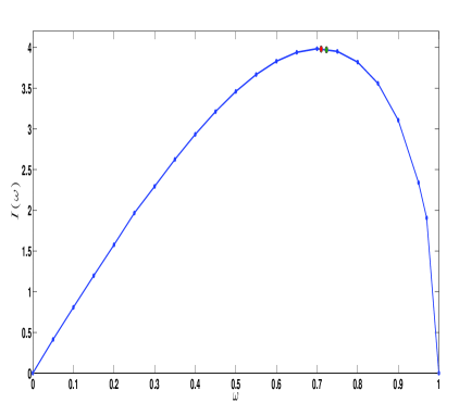
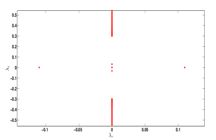
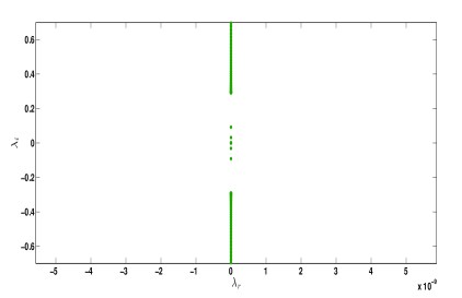
Figure 1. (a) shows the relation between $\omega$ and $I(\omega)$ when $\beta=0.06$. The red circle on the graph corresponds to $\omega=0.7$ and the green one corresponds to $\omega=0.71$. (b) shows the spectral plane $(\lambda_{r},\lambda_{i})$ of the eigenvalues $\lambda=\lambda_{r}+i\lambda_{i}$ of $\mathcal{L}$ when $\omega=0.7$ and (c) shows the spectral plane $(\lambda_{r},\lambda_{i})$ of the eigenvalues $\lambda=\lambda_{r}+i\lambda_{i}$ of $\mathcal{L}$ when $\omega=0.71$.

5. Conclusions and Future Challenges

In the present work, we have considered, motivated by $\mathcal{PT}$-symmetric considerations and perturbations respecting the parity and time-reversal symmetries, to explore a variant of the recently explored $\mathcal{PT}$-symmetric Klein-Gordon systems, which also can be thought of as a Schrödinger type equation with additional inertial terms. For this PDE, we have explored the general stability criterion of [16] in order to derive a more precise/specific stability condition. The latter has the natural form of an extension to the well-known Vakhitov-Kolokolov criterion of nonlinear Schrödinger type models. The relevant inequality has not only been theoretically proposed and directly computed in some simple case examples (such as $W(x)=1$), but its sharpness has been numerically corroborated in analytically intractable forms of the relevant function.

Nevertheless, there are numerous extensions of the present setting that may still be relevant to explore. While, partially also due to space restrictions, here we constrained ourselves and our numerical study to the prototypical cubic case, it would be interesting to explore more general (power or other e.g. saturable) nonlinearities that may well impart additional instabilities, as well as provide settings where the setup of the theorem will not apply. Here, the numerical computations may provide insights towards suitable generalizations. Also, considering more complex forms of $W(x)$ may provide multiple changes of monotonicity (of the relevant quantity of the theorem), and it would be interesting to seek the corresponding stability reversals. Finally, in the case of one or more of these instabilities, it would be useful to dynamically investigate the fate of the resulting dynamical evolutions. Such studies are presently in progress and will be reported in future studies.

References

- [1] C. M. Bender, Rep. Prog. Phys. 70 947–1018 (2007).
- [2] K. G. Makris, R. El-Ganainy, D. N. Christodoulides, and Z. H. Musslimani, Phys. Rev. Lett. 100, 103904 (2008); Z. H. Musslimani, K. G. Makris, R. El-Ganainy, and D. N. Christodoulides, Phys. Rev. Lett. 100, 030402 (2008)
- [3] H. Ramezani, T. Kottos, R. El-Ganainy, and D.N. Christodoulides, Phys. Rev. A 82, 043803 (2010).
- [4] A. Ruschhaupt, F. Delgado, and J. G. Muga, J. Phys. A: Math. Gen. 38, L171 (2005).
- [5] A. Guo, G. J. Salamo, D. Duchesne, R. Morandotti, M. Volatier-Ravat, V. Aimez, G. A. Siviloglou, and D. N. Christodoulides, Phys. Rev. Lett. 103, 093902 (2009).
- [6] C. E. Rüter, K. G. Makris, R. El-Ganainy, D. N. Christodoulides, M. Segev, and D. Kip, Nature Phys. 6, 192 (2010)
- [7] J. Schindler, A. Li, M. C. Zheng, F. M. Ellis, and T. Kottos, Phys. Rev. A 84, 040101 (2011).
- [8] H. Ramezani, J. Schindler, F. M. Ellis, U. Günther, and T. Kottos, Phys. Rev. A 85, 062122 (2012).
- [9] C.M. Bender, B.J. Berntson, D. Parker and E. Samuel, Am. J. Phys. 81, 173 (2013).
- [10] B. Peng, S.K. Ozdemir, F. Lei, F. Monifi, M. Gianfreda, G.L. Long, S. Fan, F. Nori, C.M. Bender, L. Yang, Nature Physics 10 (2014) 394.
- [11] N. Bender, S. Factor, J. D. Bodyfelt, H. Ramezani, D. N. Christodoulides, F. M. Ellis, and T. Kottos Phys. Rev. Lett. 110, 234101 (2013).
- [12] A. Demirkaya, D. J. Frantzeskakis, P. G. Kevrekidis, A. Saxena, A. Stefanov, Phys. Rev. E 88, 023203 (2013)
- [13] A. Demirkaya, M. Stanislavova, A. Stefanov, T. Kapitula, P.G. Kevrekidis, Studies Appl. Math. DOI: 10.1111/sapm.12053 (2014).
- [14] P. G. Kevrekidis Phys. Rev. A 89, 010102(R) (2014).
- [15] J. Cuevas, L. Q. English, P.G. Kevrekidis, and M. Anderson, Phys. Rev. Lett. 102, 224101 (2009).
- [16] M. Stanislavova, A. Stefanov, Physica D, 262, 1–13 (2013).
- [17] M. G. Vakhitov and A. A. Kolokolov, Radiophys. Quantum Electron. 16, 783 (1973).
- [18] M. Kwong, Arch. Rational Mech. Anal. 105, 243–266 (1989).
- [19] M. Weinstein, SIAM J. Math. Anal. 16, 472–491 (1985).
- [20] J. Shatah, Trans. Amer. Math. Soc. 290, 701–710 (1985).