Functional renormalization and mean-field approach to multiband systems with
spin-orbit coupling: Application to the Rashba model with attractive interaction
Abstract
The functional renormalization group (RG) in combination with Fermi surface patching is a well-established method for studying Fermi liquid instabilities of correlated electron systems. In this article, we further develop this method and combine it with mean-field theory to approach multiband systems with spin-orbit coupling, and we apply this to a tight-binding Rashba model with an attractive, local interaction. The spin dependence of the interaction vertex is fully implemented in a RG flow without SU(2) symmetry, and its momentum dependence is approximated in a refined projection scheme. In particular, we discuss the necessity of including in the RG flow contributions from both bands of the model, even if they are not intersected by the Fermi level. As the leading instability of the Rashba model, we find a superconducting phase with a singlet-type interaction between electrons with opposite momenta. While the gap function has a singlet spin structure, the order parameter indicates an unconventional superconducting phase, with the ratio between singlet and triplet amplitudes being plus or minus one on the Fermi lines of the upper or lower band, respectively. We expect our combined functional RG and mean-field approach to be useful for an unbiased theoretical description of the low-temperature properties of spin-based materials.
pacs:
64.60.ae, 71.27.+a, 71.70.Ej, 74.20.RpI Introduction
In the rapidly evolving field of spintronics, which aims at revolutionizing present-day computer logic and memory,Sinova and Žutić (2012) the Rashba model of a two-dimensional electron gas plays a paradigmatic rôle. By coupling the spin and orbital degrees of freedom, it provides a key to the manipulation of electron spins by means of electric fields.Barnes et al. (2014) Originally, the model was introduced in 1960 to describe the band splitting in non-centrosymmetric wurtzite semiconductors,Rashba (1960) but since then a vast number of materials have been found that are described by this model, ranging from semiconductor heterostructuresNitta et al. (1997) to the Shockley surface states of noble metalsLaShell et al. (1996); Hoesch et al. (2004) as well as noble-metal-based surface alloys incorporating heavy elements.Pacilé et al. (2006); Ast et al. (2007a, b) More recently, giant bulk Rashba spin splitting has been observed in the semiconductor BiTeI,Ishizaka et al. (2011); Bahramy et al. (2011); Schober et al. (2012) at the Te-terminated surface of bismuth tellurohalides,Eremeev et al. (2012, 2013) and in other systems based on chemical elements with high atomic numbers.Rashba (2012) These materials are promising candidates for spintronics applications such as the Datta-Das spin transistor.Datta and Das (1990) Indeed, much research is focused on the transport properties induced by the Rashba effect such as the intrinsic spin Hall effect,Sinova et al. (2004) current-driven spin torques,Miron et al. (2010) or spin precession phenomena.Wunderlich et al. (2010); Jungwirth et al. (2012)
From a many-body perspective, the equilibrium properties and in particular the low-temperature phase diagram of the Rashba model with electron-electron interactions are also of great interest. Mean-field approaches have indicated the possibility of unconventional superconductivity in the Rashba model due to the absence of the SU(2) spin rotation symmetry.Édel’shteǐn (1989); Gor’kov and Rashba (2001); Frigeri et al. (2004); Sigrist and Mineev (2012) In combination with an -wave pair potential and a sufficiently large Zeeman term, the Rashba spin-orbit coupling has been predicted to produce an effective chiral -wave superconductor carrying Majorana bound states in its vortex cores.Fujimoto (2008); Sau et al. (2010); Alicea (2010); Beenakker (2013) In a nanowire geometry, zero-energy states were then expected to appear at the two ends of the wire,Lutchyn et al. (2010); Oreg et al. (2010) a theoretical prediction which triggered the experimental hunt for Majorana fermions.Mourik et al. (2012); Williams et al. (2012)
Despite the tremendous progress in theoretical understanding, much remains to be done to identify the symmetries of the superconducting phases of the Rashba model in an unambiguous way. Mean-field solutions of the gap equation yield the superconducting order parameter from a given gap function (pair potential). For the latter, one usually assumes the absence of interband pairing, which then allows for its parametrization in terms of spin-singlet and -triplet amplitudes.Sigrist and Mineev (2012) Their ratio in turn determines the topological properties of the superconducting phase.Santos et al. (2010) It is therefore desirable to determine the gap function and the order parameter explicitly in a general setup such as the Rashba model with a local electron-electron interaction.
In this article, we address this problem for a tight-binding Rashba model on the hexagonal Bravais lattice with an attractive local interaction, using a combined functional RG and mean-field approach. The tight-binding model approximately describes the energy dispersion of the Rashba semiconductor BiTeIIshizaka et al. (2011) near the high-symmetry point of the hexagonal Brillouin zone. The attractive initial interaction induces an instability towards a superconducting phase,Bardeen et al. (1957); Thouless (1960) which can be detected by a divergence of the effective interaction vertex in the RG flow.Salmhofer and Honerkamp (2001) In real materials, an initial attractive electron interaction may typically arise, for example, from an electron-phonon mechanism.Bardeen et al. (1957); Cooper (1956) We remark that for a repulsive initial interaction, a superconducting instability generally also occurs due to the Kohn-Luttinger effect.Kohn and Luttinger (1965) However, in the absence of Fermi surface nesting, the critical scale below which the ordered phase occurs is much smaller and can therefore hardly be detected in our numerical RG approach. (For a detailed discussion of the Kohn-Luttinger effect in two-dimensional Fermi systems see Refs. Feldman et al., 1997; Sinclair, 1996, and in the context of the functional RG see Ref. Salmhofer and Honerkamp, 2001.) The superconducting instabilities in the Rashba model with a repulsive interaction have been investigated using RG methods by Vafek and Wang.Vafek and Wang (2011); Wang and Vafek (2014)
Our aim is to characterize the superconducting phases of the Rashba model with an attractive, local initial interaction without a priori assumptions on the gap form factor. For this purpose, the functional RG in combination with a Fermi surface patching approximation has proven useful.Salmhofer and Honerkamp (2001); Metzner et al. (2012) It allows to study the (possibly competing) Fermi liquid instabilities without making any potentially restrictive a priori assumptions (e.g., about the absence of interband pairing), and it yields the effective interaction for the electrons near the Fermi energy after integrating out the high-energy degrees of freedom. The RG procedure has already been successfully applied to models relevant for the high-temperature superconducting cupratesHonerkamp et al. (2001); Honerkamp and Salmhofer (2001); Husemann et al. (2012); Giering and Salmhofer (2012); Eberlein and Metzner (2014); Eberlein (2014) and iron pnictides,Wang et al. (2009); Platt et al. (2009); Thomale et al. (2009, 2011); Platt et al. (2011, 2012); Lichtenstein et al. (2014) strontium ruthenate,Wang et al. (2013) monolayer graphene,Honerkamp (2008); Kiesel et al. (2012); Wu et al. (2013); Janssen and Herbut (2014); Classen et al. (2014, 2015) bilayerScherer et al. (2012a); Lang et al. (2012); de la Peña et al. (2014) and trilayerScherer et al. (2012b) graphene, and many other correlated fermion systems (for recent reviews see Refs. Metzner et al., 2012 and Platt et al., 2013). The study of RG flow equations for non-SU(2)-invariant systems has recently become a topic of major interest.Maier et al. (2014); Scherer et al. (2014)
On the level of functional RG technique, the general set of RG equations was derived without the assumption of SU(2) symmetry in Ref. Salmhofer and Honerkamp, 2001. Our work is novel in that we fully implement the RG flow in the case without SU(2) symmetry, taking into account the full spin dependence of the interaction vertex, and using a refined projection scheme for the momentum discretization of the interaction vertex, which admits projections on the representative momenta irrespectively of the band index. In particular, we find that contributions from both bands of the model have to be included in the RG flow in order to obtain the correct effective interaction at the critical scale. Our numerical solution of the RG equations within this refined projection scheme is confirmed by an analytical resummation of the particle-particle ladder.
Furthermore, we combine our functional RG approach with mean-field theory in order to provide a more detailed characterization of the superconducting phases. While the functional RG yields the superconducting interaction at the critical scale, mean-field theory allows to predict from this the superconducting gap function and the order parameter. In particular, we generalize the Bogoliubov transformation of Ref. Sigrist and Ueda, 1991 to the non-SU(2)-symmetric case, and thereby obtain explicit expressions for the singlet and triplet amplitudes of the superconducting order parameter as a function of momentum and chemical potential. Finally, by analytically and numerically solving the scalar gap equation, we also predict the gap size as a function of the chemical potential and the interaction strength. A consistent fusion of functional RG methods and mean-field theory has already been discussed in Ref. Wang et al., 2014 (see also the earlier work Ref. Reiss et al., 2007).
The article is organized as follows: In Sec. II, we define as our starting point a minimal tight-binding model on the hexagonal Bravais lattice which displays Rashba spin splitting near the center of the Brillouin zone. In Sec. III, we introduce the functional RG and describe the Fermi surface patching approximation used
to solve the RG equations numerically. We discuss the advantages of our refined projection scheme, and after that, we present our results on the leading instabilities and corresponding effective interactions. In Sec. IV, we describe the mean-field approach used to predict the gap function and the order parameter of the Rashba model. In Appendixes A and B, we fix our conventions for the tight-binding description of electronic states on the hexagonal Bravais lattice and for the corresponding temperature Green functions. Furthermore, Appendix A contains an elementary derivation of our minimal tight-binding model from symmetry conditions only, and Appendix B a brief review of the most important definitions and properties of temperature Green functions. These two appendixes are essentially self-contained and can be read independently as pedagogical reviews. Finally, in Appendix C we derive the projected RG equations which we have implemented numerically, and we show how the mean-field interaction is deduced from the resulting projected interaction vertex.
II Rashba model with local interaction
We study a minimal tight-binding model on the hexagonal Bravais lattice in two dimensions, which displays Rashba spin splitting near the center of the Brillouin zone. The free Hamiltonian is given by
| (1) |
Here, the Bloch momentum ranges over the (first) Brillouin zone , and we use a normalized measure
| (2) |
where is the area of the Brillouin zone. Furthermore, are spin indices. For a more detailed exposition of our conventions, see Appendix A.1. We can expand the Hamiltonian matrix as
| (3) |
where denotes the identity matrix and the vector of the Pauli matrices. In terms of the dimensionless quantity
| (4) |
where denotes the lattice constant, the coefficient functions of our minimal tight-binding model are given explicitly by
| (5) | ||||
| (6) | ||||
| (7) | ||||
| (8) |
where and are constants. In Appendixes A.2–A.3, we show that this model corresponds in direct space to nearest-neighbor hopping with the amplitudes and , and that this model can be derived from symmetry considerations only. The constant term has been added to the Hamiltonian such that (and consequently both eigenvalues at are zero). Since , the model Hamiltonian (3) is not invariant under general SU(2) spin rotations. For small momenta, we can Taylor expand the above functions to quadratic order in the momentum as
| (9) | ||||
| (10) | ||||
| (11) | ||||
| (12) |
This shows that near the center of the Brillouin zone, the model is described by the Rashba Hamiltonian
| (13) |
This can be written equivalently as
| (14) |
where the Rashba energy and the Rashba wave vector are related to the parameters of the tight-binding model by
| (15) |
The characteristics of the Rashba model dispersion are (i) the band crossing at , (ii) the approximately linear dispersion for small wave vectors, and (iii) the band minimum which is attained on the circle around the axis of symmetry.Boiko and Rashba (1960) The Rashba energy , which equals the energy difference between the band crossing and the band minimum, is often used to quantify the Rashba spin splitting of the energy bands in real materials.Ishizaka et al. (2011) In the following, we define all quantities with the dimension of an energy by specifying their ratio to the hopping parameter . In particular, we choose the model parameter such that
| (16) |
Now, we come to the diagonalization of the Hermitian matrix (3). Generally, we have
| (17) |
where are band indices, and the eigenvalues are given by
| (18) |
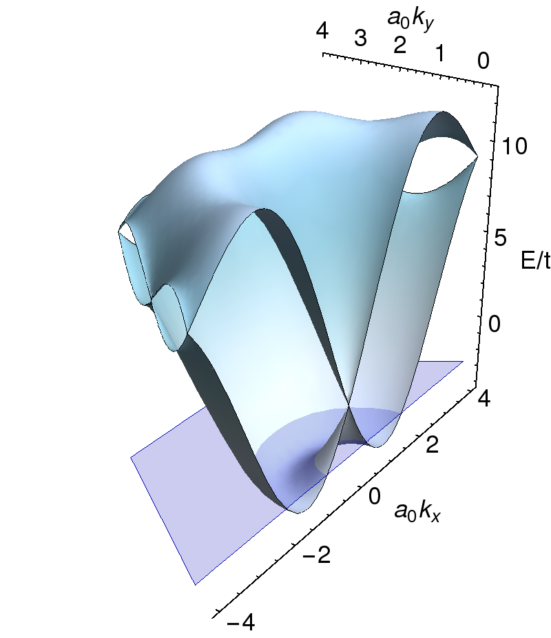
We refer to and as the lower and the upper energy band, respectively. Their dispersion is shown in Fig. 1. The unitary matrix mediates between the spin basis and the band basis. It contains the normalized eigenvectors as column vectors and is given by
| (21) | |||
| (24) |
where we have suppressed the dependencies on the right-hand side of the equation. Furthermore,
| (25) |
and is defined by
| (26) | ||||
| (27) |
Equivalently, we can write this as
| (28) |
Note that is not the polar angle of the vector , but of the vector . Since in our model, the unitary matrix (24) simplifies to
| (29) |
The density of states (DOS) is defined separately for each energy band as
| (30) |
while the total DOS is defined by their respective sum,
| (31) |
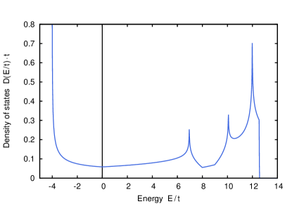
The total DOS of the minimal tight-binding model is shown in Fig. 2. In particular, we read off the bandwidth (i.e. the difference between the band maximum and the band minimum) of the model,
| (32) |
For the ideal Rashba Hamiltonian (14), the DOS can be calculated analytically and is given by (see e.g. Ref. Winkler, 2003, Eqs. (6.20a)–(6.20b))
| (33) | ||||
This function has the following properties: (i) it is constant for , (ii) it is continuous but has a kink at the band crossing (where ), and (iii) it diverges at the minimum of the lower band, .
In addition to the quadratic Hamiltonian (1), we consider a quartic interaction term of the form
| (34) | ||||
which is a shorthand notation for Eq. (443). In particular, is fixed by Bloch momentum conservation,
| (35) |
where the reciprocal lattice vector ensures that lies in the first Brillouin zone. We choose a momentum-independent interaction kernel,
| (36) |
The corresponding operator then coincides with the normal-ordered operator
| (37) | ||||
| (38) |
where the spin-resolved density operator is defined as
| (39) |
An interaction of the form (37) is called local, because it contains only products of electronic density operators at the same lattice site. We choose the parameter as
| (40) |
In particular, the negative sign means that we consider an attractive interaction between electrons. The interaction (36) is SU(2) invariant. The interaction kernel in the band basis is defined in terms of its counterpart (36) in the spin basis by
| (41) | ||||
with given by Eq. (29). For momentum combinations with , and hence by Eq. (35) also , we obtain the following explicit expression
III Functional renormalization group
III.1 RGE without spin rotation invariance
To obtain the phase diagram of the Rashba model, we use the functional RG approach which describes the evolution from the initial interaction at the ultraviolet scale to an effective interaction at low energies.Metzner et al. (2012) Importantly, this method accounts for the interplay between different ordering tendencies in an unbiased way. Explicitly, we employ the fermionic RG for the one-line irreducible Green functions with a momentum cut-off as introduced in Ref. Salmhofer and Honerkamp, 2001. The generating functional for the one-line irreducible Green functions is the Legendre transform of the generating functional for the connected Green functions (see Appendix B). To induce the RG flow, we modify the free two-point Green function of the model by introducing an infrared regulator suppressing modes with energies less than a scale . This leads to a scale dependence of the generating functional, , and a hierarchy of renormalization group equations (RGE) for the one-line irreducible Green functions. The resulting RG flow smoothly interpolates between the initial interaction defined at the ultraviolet scale and the low-energy effective interaction for .
In the truncation of the hierarchy used here, typical RG flows then show the following behavior: As the energy scale is lowered, the effective two-particle interaction diverges already at a nonzero critical scale for particular combinations of momenta and further indices such as spins or bands. This is interpreted as a signal for “an instability leading to an ordered phase via spontaneous symmetry breaking” (Ref. Reiss et al., 2007; see also Ref. Kohn and Luttinger, 1965, footnote 2). The divergence of the effective interaction is due to the truncation, which in particular restricts to the symmetric phase. It has been shownSalmhofer et al. (2004); Gersch et al. (2005) that the flow can be continued into the symmetry-broken phase and down to if the symmetry-breaking terms indicated by the effective interaction above are included. The level-two truncation is therefore not used down to , but the flow is stopped at a scale where the coupling reaches a certain threshold (but is still finite). This can be justified in a certain scale range depending on the Fermi surface curvature.Salmhofer and Honerkamp (2001) From the momentum structure of the near-critical two-particle interaction at one can then construct an effective low-energy Hamiltonian and determine the leading Fermi liquid instability. The effective interaction just above is often referred to as “the interaction at .” We will also follow this slightly loose convention below, but note here that more strictly, this is to mean “the interaction at .”
In the following, we will give explicit expressions for the RG equations in our model. We use the conventions described in Appendix B. The free two-point Green function (or covariance) in the spin basis, which is defined as the Fourier transform of Eq. (462) with respect to the spatial variables, obeys the equation of motion
| (45) | ||||
where has been defined by Eqs. (3)–(8). This can be shown directly from the imaginary-time analog of the Heisenberg equation of motion for the field operators,
| (46) |
where denotes the particle-number operator. In the frequency domain, Eq. (45) is equivalent to (see Eqs. (454)–(455))
| (47) | ||||
The covariance in the band basis is defined by means of the unitary matrix (see Eq. (17)) as
| (48) |
It obeys the equation of motion
| (49) |
and is therefore given explicitly by
| (50) |
Here and in the following, we denote by
| (51) |
the eigenvalues of the single-particle Hamiltonian measured from the chemical potential.
The scale-dependent covariance is now defined in the band basis by
| (52) |
where denotes the regulator function. The latter can be chosen either as a strict cut-off function, which is a smooth function with the properties that
| (53) |
For this choice, the numerator of Eq. (52) vanishes if
| (54) |
which means that all momenta inside a shell of thickness around the Fermi lines are cut off. For the concrete implementation of the RG equations, we will use instead the regulator function
| (55) |
This is always greater than zero and smaller than one, hence Eq. (53) holds only up to terms of the order . Correspondingly, in Eq. (52) all momenta inside a shell of thickness around the Fermi lines are suppressed (but not cut off). We will, however, do our calculations at a tiny positive temperature (such that ), where can be used down to scales .
The meaning of the regulator function can most easily be explained by referring to the strict cut-off function: The scale-dependent covariance (52) approaches the original free two-point Green function in the infrared limit,
| (56) |
Furthermore, by defining the ultraviolet scale (or initial scale) much larger than the bandwidth of the model, such that
| (57) |
the covariance vanishes at this scale, i.e.,
| (58) |
Now, the scale dependence of the covariance induces by means of the Feynman graph expansion a scale dependence of all interacting temperature Green functions. In particular, the one-line irreducible Green functions (see Appendix B.4) become scale dependent,
| (59) |
Again, the infrared limit simply yields back the original one-line irreducible Green functions: for ,
| (60) |
Here and in the following,
| (61) |
denotes a multi-index composed of the lattice site , the spin variable and the imaginary-time variable . On the other hand, at the ultraviolet scale , the one-line irreducible two-point function is not well defined. This is because is the inverse of the (full) two-point Green function (see Eqs. (477) and (483)), but the covariance and hence also vanish identically at the ultraviolet scale. For , the one-line irreducible Green functions can still be defined at the ultraviolet scale, because the inverse of does not appear in their Feynman graph expansions (see Appendix B.4). In particular, for we obtain 111Note the prefactor in Eq. (62): The factor 2 comes from the fact that there are indeed two first-order Feynman graphs contributing to (see Table 7), while appears as a prefactor of every -th order Feynman graph. In particular, both sides of Eq. (62) have the same dimension, because by our conventions the interaction kernel has the dimension of an energy, whereas all Green functions are dimensionless (see Appendix B).
| (62) |
where is the interaction kernel given by
| (63) | |||
(see Appendix B.2), and where
| (64) | |||
is the inverse Fourier transform of Eq. (36). Furthermore, for we have
| (65) |
because all Feynman graphs contributing to contain at least one internal line carrying the covariance .
![[Uncaptioned image]](/html/1409.7087/assets/x2.png)
|
The RG equations in the one-line irreducible scheme constitute an infinite hierarchy of coupled differential equations, which is exactly solved by the scale-dependent one-line irreducible Green functions (see Ref. Salmhofer and Honerkamp, 2001). In practice, this hierarchy has to be truncated in order to allow for approximate solutions. Our above-mentioned standard truncation is the level-two truncation, where one keeps only the two- and the four-point function in the flow and sets
| (66) |
The RG equations in the level-two truncation read explicitly as follows: For ,
| (67) | ||||
Here, the dot denotes the derivative with respect to the scale parameter . Furthermore,
| (68) |
is the inverse of the scale-dependent covariance, and is the single-scale Green function. The latter is defined in terms of and the scale-dependent (full) two-point Green function as the operator product
| (69) |
In terms of integral kernels, this means
| (70) | ||||
where the integrations over multi-indices (see Eq. (61)) are defined as
| (71) |
For , the RG equation in the level-two truncation reads as
| (72) | ||||
where the three terms on the right-hand side are called the particle-particle term, the crossed particle-hole term and the direct particle-hole term. These three terms are given explicitly by
| (73) | ||||
| (74) | ||||
| (75) |
Here, the loop function is defined in terms of the full two-point Green function and the single-scale Green function by
| (76) | ||||
Graphically, the RG equations (67) and (72) are represented by means of universal Feynman graphs in Table 1 (see Ref. Starke and Kresse, 2012, and Table 7 for our conventions).
In order to simplify the RG equations, we first switch to the Fourier domain, where the above equations (67)–(76) hold in precisely the same form but with the multi-indices replaced by
| (77) |
Here, ranges in the first Brillouin zone , and is a fermionic Matsubara frequency (see Appendix B.1). Then, the summations over get replaced by integrations over , and the -integrals get replaced by summations over the Matsubara frequencies, i.e.,
| (78) |
We further employ translation invariance, which effectively reduces the number of arguments of all Green functions by one (see Appendix B.1). Next, we switch from the spin basis to the band basis by means of the unitary matrix from Sec. II. For example, the four-point function in the band basis is defined in terms of its counterpart in the spin basis by (cf. Eq. (41))
| (79) | ||||
Furthermore, we employ the following approximations to the RG equations (besides the level-two truncation), which have already been established in many works before:Metzner et al. (2012); Platt et al. (2013) We neglect the self-energy , which is defined by the equation (cf. (482))
| (80) |
This means, we replace the full two-point Green function by the covariance . Thus, the RG equation for the four-point function becomes closed and decouples from the equation for . The single-scale Green function simplifies to
| (81) |
and the loop function becomes (in a symbolic notation)
| (82) |
Moreover, we neglect the frequency dependencies of the four-point function, i.e., we replace
| (83) | ||||
This approximation in combination with the choice of a momentum regulator (see Eq. (52)) allows us to perform the remaining frequency sums on the right-hand side of the RG equations analytically and thereby to obtain explicit expressions for the particle-particle and particle-hole loops (see Eq. (90) below). Finally, we reformulate the RG equation in terms of the scale-dependent effective interaction (or interaction vertex) , which is related to the one-line irreducible four-point Green function by
| (84) |
From this definition and from Eq. (62), we see that the initial condition for at the ultraviolet scale is precisely given by the original interaction kernel,
| (85) |
The latter is given in the spin basis by Eq. (36) and in the band basis by Eq. (41). With these simplifications, the RG equations for the interaction vertex read as follows:
| (86) | ||||
where the particle-particle term, the crossed particle-hole term, and the direct particle-hole term are given bySalmhofer and Honerkamp (2001)
| (87) | ||||
| (88) | ||||
| (89) |
In these equations, the particle-particle loop , and the particle-hole loop are given by
| (90) |
with the functions defined by
| (91) |
and respectively
| (92) |
Recall that are the eigenvalues of the single-particle Hamiltonian measured relative to the chemical potential. Furthermore,
| (93) |
denotes the Fermi distribution function, which in the zero-temperature limit reduces to
| (94) |
(except at ), where denotes the Heaviside step function. Note that in Eqs. (87)–(89), the reciprocal lattice vector is fixed in each term by the condition that all external momenta and all internal momenta lie in the Brillouin zone . The vector is then fixed by the Dirac delta distribution, and hence the right-hand side of the RG equation effectively requires only a summation over two band indices and an integration over one Bloch momentum .
The initial value problem for the scale-dependent interaction vertex is defined by the RG equation (86) and the initial condition (85). This initial value problem has a unique solution, which, however, may typically not be continued down to . In fact, as mentioned above, the interaction vertex diverges already at a nonzero scale , signaling an instability towards an ordered phase. We define the stopping scale (which is greater, but close to ) as the scale where the supremum of exceeds a certain threshold value . More precisely, with the scale-dependent vertex supremum
| (95) |
we define the stopping condition for the RG flow as
| (96) |
The effective interaction at the stopping scale can then be transformed back into the spin basis by using the unitary matrix from Sec. II, i.e.,
| (97) |
III.2 Fermi surface patching approximation
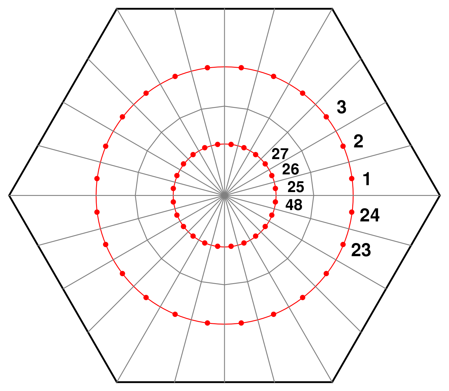
In order to solve the RG equations numerically, we discretize the momentum dependence of the interaction vertex . A standard approximation is Fermi surface patching, where each momentum is projected on a representative momentum on the Fermi surface (or Fermi line in two dimensions).Salmhofer and Honerkamp (2001); Metzner et al. (2012) By projecting the three momentum arguments of the interaction vertex to the Fermi line, the RG equations can be reformulated in terms of finitely many parameters. For one-band systems, this fixes the projection unambiguously, whereas for multiband systems, one still has to specify the dependence on the band indices. In this work, we use a refined projection scheme that makes no assumption on the relative importance of the contributions from different bands.
To explain this in more detail, we choose for each band intersected by the Fermi level a number of representative momenta , , which lie on the respective Fermi line of the band . Furthermore, we denote by
| (99) |
the total number of representative momenta, and let
| (100) |
be an index which labels all representative momenta (on all Fermi lines). This means, we identify
| (101) | ||||
In our refined projection scheme, we divide the Brillouin zone into disjoint patches,
| (102) |
where the patch is defined as the set of all momenta in which lie closer to the representative momentum than to any other representative momentum (see Fig. 3). We then make the following ansatz, which assumes the interaction vertex in the band basis to be constant on each patch:
| (103) | ||||
where is the characteristic function defined by
| (104) |
and where is approximated patch-wise by its value at the representative momenta, i.e.,
| (105) |
Thus, we are left with a finite set of parameters for the interaction vertex labeled by four band indices and three patch indices . Now, for each fixed combination of band indices, the projected interaction vertex (103) gets contributions from combinations of representative momenta. For example, the representative momentum may lie on the Fermi line of any band , i.e., not necessarily . Therefore, if denotes the number of bands (in our case ), there are in total complex numbers—given by Eq. (105)—which parametrize the interaction vertex.
For a clearer comparison, let us contrast our projection scheme with the projection scheme described, e.g., in Ref. Platt et al., 2013: There, one divides the Brillouin zone for each band separately into disjoint patches,
| (106) |
Each representative momentum lies on the Fermi line of the band within the patch . One then parametrizes the interaction vertex as follows:
| (107) | ||||
where
| (108) | ||||
Now, for each fixed combination of band indices, the projected interaction vertex (107) gets contributions from only combinations of representative momenta. For example, in Eq. (108) necessarily lies on the Fermi line of the band . If the fourth band index is not further specified (and hence allowed to take values in each band of the model), then this projection scheme leaves complex numbers parametrizing the interaction vertex. If is fixed by another condition (e.g. by requiring that is the representative momentum with the smallest distance to ), then even only parameters of the interaction vertex remain. This is by a factor of smaller than the number of parameters in our refined projection scheme.
For the Rashba model considered in this article, however, it turns out that all parameters of the discretized interaction vertex need to be considered in the RG flow. This means, only the refined projection ansatz (103) yields a meaningful approximation to the exact solution of the initial value problem described in the previous subsection (the RG equation (86) together with the initial condition (85)). By contrast, the ansatz (107) with a reduced number of parameters leads to a qualitatively different result for the effective interaction (see the discussion in the following subsections III.3–III.5).
Finally, we derive the explicit RG equations for the discretized interaction vertex in the refined projection scheme, which can be directly implemented numerically (see Appendix C.1). By putting our ansatz (103) into Eqs. (86)–(89), we obtain the following approximate equations for the finitely many parameters of the interaction vertex:
| (109) | ||||
where the three terms on the right-hand side are, respectively, given by
| (110) | ||||
| (111) | ||||
| (112) |
Here, we have defined
| (113) | ||||
with the functions defined by Eqs. (91)–(92). Note that in the particle-particle term (110), the reciprocal lattice vector is fixed by the condition
| (114) |
and therefore depends on only three patch indices , , and . The stricter condition
| (115) |
then also fixes the patch index . Hence, the right-hand side of Eq. (110) effectively requires only the summation over two band indices and one patch index . The same applies to the particle-hole terms.
In our numerical implementation, we have directly solved the RG equations (109)–(112) for the discretized interaction vertex. The solution with the given initial interaction can formally be written as
| (116) | ||||
| (117) |
The scale integral has been performed numerically by starting at the initial scale and stepwise determining from the previously calculated . The integration steps have been adjusted in each step depending on how fast the interaction vertex changes in the flow. In this way, the divergence at the critical scale could be approached numerically by gradually decreasing the step size. We remark that our implementation for the Rashba model uses patch momenta, on each of the two Fermi lines as shown schematically in Fig. 3. We have checked that our results do not change significantly by further increasing the number of patches, i.e., by taking 72 instead of 48 patches.
III.3 Effective superconducting interaction
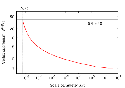
As described above, we have numerically solved the discretized RG equations (109)–(112) with an attractive onsite interaction at the initial scale . The latter was chosen much larger than the bandwidth of the model (given by Eq. (32)), i.e.,
| (118) |
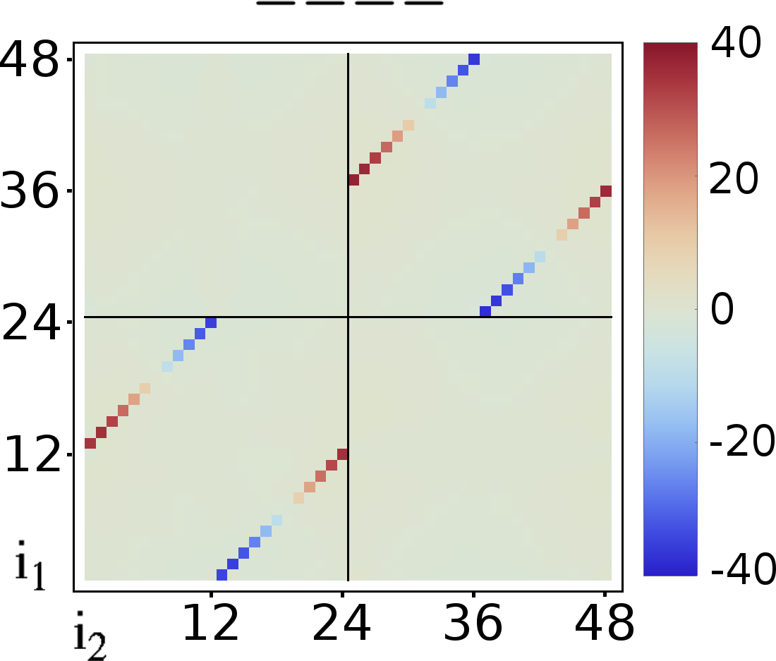
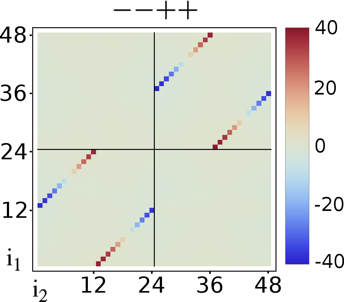
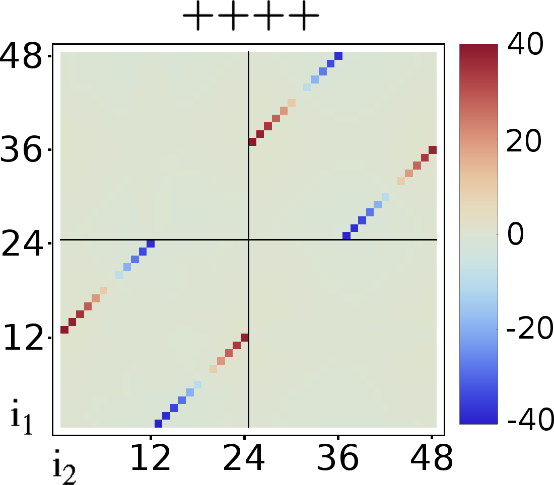
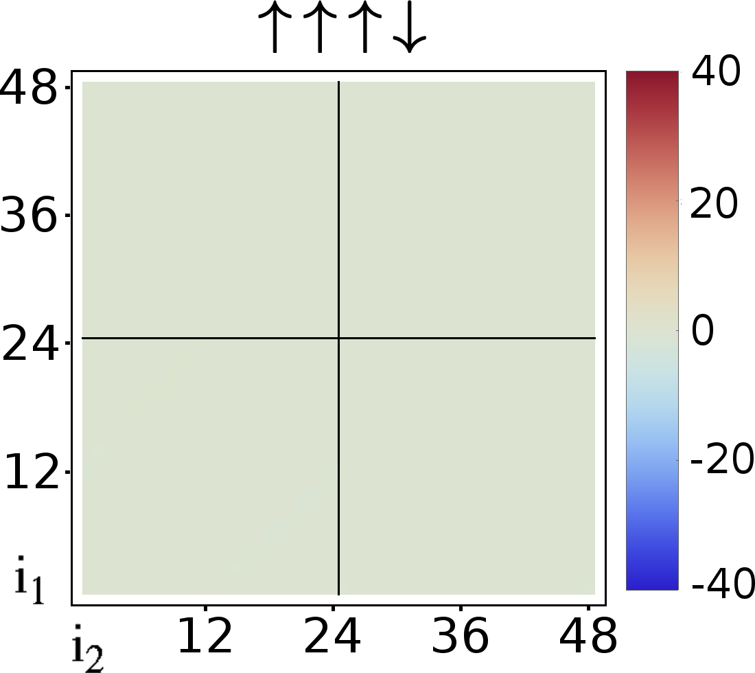
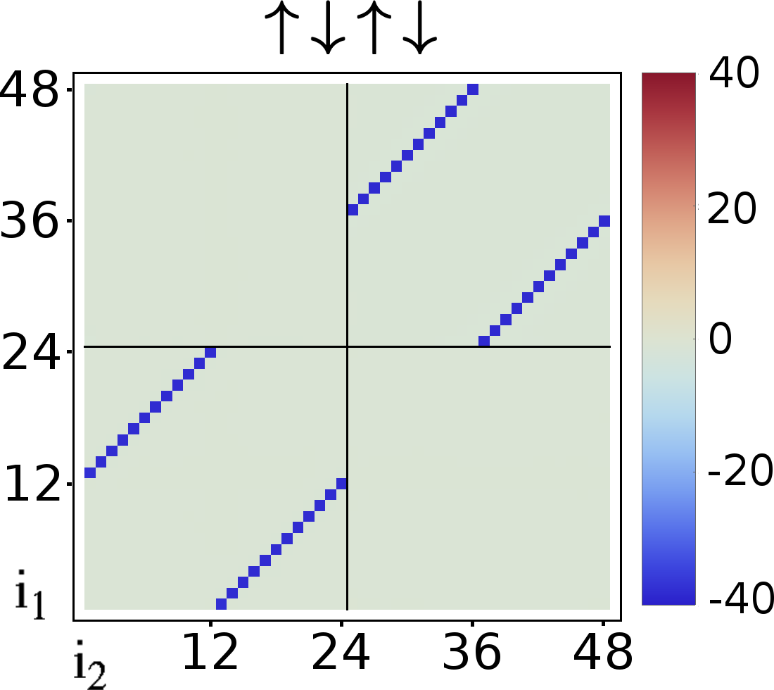
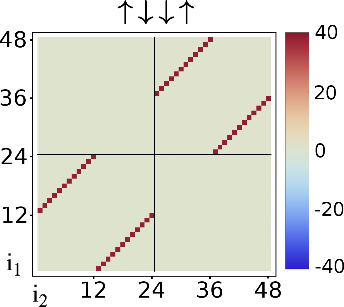
Thus, the condition (57) is fulfilled, and our results do not change by further increasing . We have stopped the RG flow at the stopping scale defined by Eq. (96), which is close to the critical scale where the interaction vertex diverges. (As mentioned above, in the following, we do not distinguish explicitly between these two scales.) Our numerical result for the vertex supremum as a function of the scale parameter is shown in Fig. 4. One clearly sees that the interaction vertex grows with decreasing and eventually approaches a divergence at the critical scale. The numerical result for the effective interaction at the stopping scale is shown in the band basis in Fig. 5 and in the spin basis in Fig. 6. We have fixed the third patch index and analyzed the dependence of the effective interaction on and for all possible band and spin combinations (of which four representative ones are shown in Figs. 5 and 6, respectively). The result clearly signals a superconducting instability, where pairing occurs between opposite momenta on the same Fermi line. The discretized effective interaction at the stopping scale is well represented in the band basis by
| (119) | ||||
and in the spin basis by
| (120) | ||||
where is the threshold parameter (see Eq. (98)). The corresponding interaction operator (which is obtained by inserting Eq. (120) into the projection ansatz (103)) is then approximately given by
| (121) | ||||
where is the number of patches. The factor corresponds to the area of a single -space patch, which arises because our effective interaction (120) turns out to have a restriction on the level of patches (see the derivation in Appendix C.2). By explicitly performing the spin sums and using the canonical anticommutation relations of the creation and annihilation operators, we further obtain the equivalent expression
| (122) | ||||
where we have defined the coupling constant
| (123) |
The interaction (122) is a singlet superconducting interaction. We have obtained this result for the effective interaction at the critical scale independently of the chemical potential , whether it is above () or below () the band crossing of the Rashba dispersion.
We stress that the form of the effective interaction crucially depends on the projection scheme used to discretize the scale-dependent interaction vertex (see Sec. III.2). Our result given by Eqs. (119)–(120) has been obtained by using the refined projection scheme, while a qualitatively different result would be obtained in the projection scheme of Ref. Platt et al., 2013. The reason for the difference between the two projection schemes can in fact already be understood by considering the discretized initial interaction. The latter is given in the spin basis by (see Eq. (36))
| (124) |
and in the band basis by
| (125) | ||||
where is defined by the condition
| (126) |
with some reciprocal lattice vector . For momentum combinations where , and consequently also , we obtain the following explicit expression (analogous to Eq. (42)):
| (127) | ||||
Now, let be a representative momentum, say, on the Fermi line of the band . Furthermore, let be the opposite momentum on the same Fermi line. Then, Eq. (127) implies that
| (128) |

Hence, the two components of the discretized interaction vertex with or are equal in magnitude. For each representative momentum on the Fermi line of the band , one therefore has to take into account both components and of the discretized interaction (not only those with ). Furthermore, if we transform Eq. (127) back to the spin basis by
| (129) |
we recover again the initial interaction (124). Thus, the transformation of the discretized interaction between the band basis and the spin basis is exact in the refined projection scheme. On the other hand, if we neglected all components in Eq. (127) with (where is the band index of the representative momentum ), then we would lose information on the interaction kernel, and by transforming the result back to the spin basis we would obtain a qualitatively different interaction.
Our numerical implementation of the RG equations further shows that the property (127) remains unchanged in the flow, i.e., the scale-dependent interaction vertex has this property for every (and in fact near the critical scale, all other contributions with become negligible). This is most clearly seen in Fig. 5, which shows the four contributions
| (130) | ||||
of the interaction vertex in the band basis at the stopping scale . The four contributions are of equal magnitude, and the momentum dependence is well described by Eq. (119). We emphasize that this comes out even in the case where the chemical potential is in the lower band ( in Fig. 5), which implies that the upper band is completely empty (at ). The unexpected result that even in this case contributions to the interaction vertex with an upper band index cannot be neglected in RG flow will be explained further by means of an analytical resummation of the particle-particle ladder in Sec. III.5.
III.4 Critical scale and phase diagram
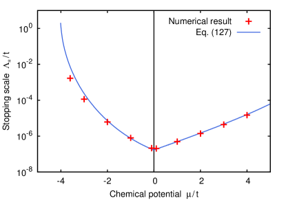
The RG flow is stopped at the scale where the vertex exceeds a threshold value and hence a divergence is approached, which signals the breakdown of the Fermi liquid description. Figure 7 shows as a function of the chemical potential . The numerical data turns out to be well represented by the following formula:
| (131) |
where is the initial interaction strength (given by Eq. (40)), and is the density of states of the minimal tight-binding model as shown in Fig. 2. The exponent in this formula can in fact be motivated by an analytical resummation of the particle-particle ladder as performed in the next subsection (see the text following Eq. (155)). In particular, the sharp increase of for small reflects the diverging density of states at the band minimum of the Rashba dispersion, and the kink at corresponds to the kink in the density of states at the band crossing (cf. Eq. (33) for the ideal Rashba model).
We stress again that the choice of the momentum projection scheme has a strong impact on the simulational result for the form of the effective interaction near the critical scale, and even for the critical scale itself. In fact, the characteristic dependence of the critical scale on the density of states as shown in Fig. 7—and described by Eq. (131), which is consistent with the particle-particle ladder resummation—could only be reproduced in our refined projection scheme. We conclude that it is imperative to include all parameters of the interaction vertex in the RG flow, i.e., to use the refined projection scheme, in order to obtain the correct results for the effective interaction and the critical scale in our model. It would be interesting to compare the two projection schemes (described in Sec. III.2) also for other models with several bands, in order to see whether their difference is a special feature of the Rashba model or a general issue to be considered in the Fermi surface patching approximation for multiband systems.
We conclude this subsection with a remark about the interpretation of Fig. (7) as a “phase diagram.” In two dimensions, the critical scale can be regarded as an estimate for a true temperature of a phase transition, in which the ordering sets in, in the following sense: In cases where the symmetry that gets broken is discrete, the breaking is strictly allowed. When, as in our case, a continuous symmetry is involved, no long-range order can exist in an infinite two-dimensional system due to the Mermin–Wagner theorem. However, for a finite (large) system, a sufficiently slow decay of correlations becomes indistinguishable from long-range order. Moreover, in the case of three-dimensional materials with a layered structure such as BiTeI, correlated fermion models have a much smaller hopping amplitude in the direction perpendicular to the layers than in the layers, but a slow decay of correlations in a single layer means that the order-parameter field is almost constant in large domains of the layer. The typical area of these domains can then scale up even small interlayer couplings between the order-parameter fields, hence at some low temperature make the dynamics three-dimensional so that ordering can set in. Finally, we note that mean-field theory yields a quantitative relation between the critical scale and the critical temperature , which is obtained from the gap equation by assuming that the superconducting gap vanishes as the temperature approaches (see Eq. (248) in Sec. IV.4).
III.5 Particle-particle ladder resummation
In our numerical evaluation of the RG equations for an initial attractive, local interaction, the particle-hole terms remain small, and the full RG flow is close to the result of a particle-particle ladder resummation (see Ref. Salmhofer, 1999, Sec. 4.5.4). Therefore, we restrict ourselves in the following to the particle-particle flow. We first give a heuristic argument which shows that when a superconducting instability is approached, the scale-dependent interaction vertex has relevant contributions from both bands of the model even if the Fermi level intersects only the lower band (such that the upper band is empty at ). After that, we provide a general analytical solution of the particle-particle flow in the spin basis, which applies to the case where the single-particle Hamiltonian is not SU(2) invariant. This solution is consistent with our numerical results as presented in the previous subsections.
The particle-particle flow for the discretized interaction vertex is defined by the RG equation (109) where only the particle-particle term (110) is kept on the right-hand side. Thus, we consider the equation
| (132) | ||||
with given by Eq. (113). A special solution of this equation is a superconducting interaction of the form
| (133) | ||||
in the spin basis, or
| (134) | ||||
in the band basis (cf. Eqs. (119)–(120)). Here, is a scale-dependent coupling parameter. By putting this ansatz into Eq. (132), we obtain the differential equation
| (135) |
where we have defined for ,
| (136) | ||||
with . Before coming to the solution of Eq. (135), we simplify the above expression. We use that by time-reversal symmetry,
| (137) |
and, furthermore,
| (138) |
Thus, we obtain
| (139) | ||||
In the zero-temperature limit, , this yields
| (140) |
This expression can be written as a scale derivative,
| (141) |
of the function
| (142) |
Further defining
| (143) |
we can write Eq. (135) as
| (144) |
The unique solution of this differential equation with the initial condition
| (145) |
is now given by
| (146) |
To obtain an even more concrete expression, we replace the regulator function by a sharp cut-off function, i.e.,
| (147) |
This has the property , and its scale derivative is given by
| (148) |
From Eqs. (141)–(142), we therefore obtain
| (149) |
(For the general treatment of the sharp cut-off limit, see the Appendix of Ref. Honerkamp and Salmhofer, 2003.) In terms of the densities of states of each band (defined by Eq. (30)), we can further write Eq. (149) as
| (150) |
This expression approaches
| (151) |
as , if is regular at . The singular term can be integrated explicitly to yield
| (152) |
Thus, the solution (146) turns into
| (153) |
where is the total density of states. In particular, diverges at a critical scale , which is determined through the equation
| (154) |
and given explicitly by
| (155) |
This result can already be compared with our numerical result for the stopping scale shown in Fig. 7. However, since Eq. (155) has been derived by solving the particle-particle flow in the limit , we cannot expect an exact agreement with our numerical solution, which had been obtained by starting the RG flow at an initial scale much larger than the bandwidth of the model. Nevertheless, it turns out that the formula (131) agrees well with our numerical data. This is obtained from Eq. (155) by identifying with the strength of the initial onsite interaction and replacing the prefactor by a numerical factor (which in the logarithmic plot corresponds to a constant shift of the whole curve).
It is now instructive to consider an ansatz for the solution of Eq. (132) which is more general than Eq. (134), namely
| (156) | ||||
with a matrix of generalized coupling parameters. In the following, we will suppress the dependencies in the notation. Hermiticity requires that
| (157) |
such that are real and . For the particular choice
| (158) | ||||
| (159) |
we recover again the superconducting interaction (134). We focus on the case where the chemical potential is in the lower band, such that
| (160) |
and the total density of states is determined only by the lower band,
| (161) |
Naïvely, one could expect that in this case only the coupling is important in the flow, while all couplings with at least one upper band index do not play any rôle. We will now show, however, that this is not true.
By putting the generalized ansatz (156) into the RG equation (132), we obtain after a straightforward calculation the following coupled differential equations for the generalized coupling constants:
| (162) |
or equivalently,
| (163) | ||||
| (164) | ||||
| (165) |
with the coefficient functions , given by Eq. (136). By our result (151), the vanishing of also implies
| (166) |
and hence the above system simplifies to
| (167) | ||||
| (168) | ||||
| (169) |
Let us assume that at some initial scale we have the equalities
| (170) |
The second equation (168) is closed and can be solved readily: with the above initial condition, we find
| (171) |
precisely analogous to Eq. (153). Next, consider the equation (169) for the coupling . The point is now that also appears on the right-hand side of this equation, and thereby drives the flow of . In particular, as , the growing of also leads to a divergence of . Concretely, the solution of Eq. (169) with the initial condition (170) is simply
| (172) |
Similarly, we see from Eq. (167) that drives the flow of , and in the end we obtain the solution
| (173) |
Thus, we have shown that all couplings remain of equal magnitude in the flow and together approach a divergence as , even though the upper band is completely empty. In other words, if the condition (170) is satisfied at some initial scale , then this property of the effective interaction remains invariant in the particle-particle flow.
Finally, we generalize the above heuristic argument in order to provide an analytical solution of the particle-particle flow for a general class of SU(2)-symmetric initial interactions. For this purpose, we switch to the spin basis, where the particle-particle flow equation reads as (cf. Eqs. (86)–(87) in the band basis)
| (174) | ||||
Note that the particle-particle loop in the spin basis depends on four spin indices and is given in terms of its counterpart in the band basis, Eq. (90), by
| (175) |
We assume that the initial interaction is SU(2) invariant and of the following form:
| (176) | ||||
or more precisely,
| (177) | ||||
with an arbitrary function . For example, an onsite attractive interaction corresponds to
| (178) |
with , while a superconducting interaction is represented by
| (179) |
with . Now, given any initial interaction of the form (176), one can show that the effective interaction retains this form in the particle-particle flow. In particular, this means that the SU(2) invariance of the effective interaction is preserved in the particle-particle flow even if the single-particle Hamiltonian does not possess this symmetry. This can be proven easily by putting the ansatz (176) into the RG equation (174) and using the identity
| (180) |
(see Ref. Édel’shteǐn, 1989, Eq. (10)). The RG equation for the interaction vertex then reduces to a decoupled system of differential equations, one for each component with . Explicitly, this reads as
| (181) |
where the coefficient functions are given by
| (182) | ||||
A straightforward calculation using Eq. (175) and the property (44) of the unitary matrix further yields
| (183) | ||||
In particular, for , we have
| (184) |
and hence,
| (185) | ||||
| (186) |
with the functions defined by Eq. (136). The differential equation for the component is therefore equivalent to the flow equation for the coupling constant of a superconducting interaction (see Eq. (135)). Furthermore, the general solution of Eq. (181) with the initial condition
| (187) |
is given by
| (188) |
which generalizes the result (146) derived above for a superconducting interaction. In principle, Eq. (188) can be used to determine the flow of the interaction vertex from the attractive onsite interaction at the initial scale to the superconducting interaction at the critical scale.
Our final remark in this section regards the question of why it is sufficient (for our model) to choose all the representative momenta on the Fermi lines (of any band) instead of taking a two-dimensional grid of discrete momenta in the whole Brillouin zone: From the expressions (90)–(92), one can see that the loop terms are singular if both and lie on the Fermi lines of the respective bands and , such that . This motivates a simplification of the momentum dependence of the interaction vertex by a projection to the Fermi lines. The quality of this approximation has been discussed for the different RG schemes in Refs. Salmhofer, 1998; Halboth and Metzner, 2000; Salmhofer and Honerkamp, 2001; Metzner et al., 2012. The fact that the projected vertex function is constant along paths transversal to the Fermi lines, hence may become large also away from the Fermi lines, usually leads to a slight overestimation of the coupling functions, hence a more conservative estimate of the stopping scale. The particle-particle flow considered here provides an example where the coupling function really is constant along certain lines in momentum space. In our analytical solution, Eq. (176) with given by Eq. (188), the flow coefficients are largest when the external momenta satisfy , which does not restrict and to the Fermi lines. In fact, this analytical solution is even independent of the distance of or from the Fermi lines.
IV Mean-field theory
IV.1 Definitions
By starting from an attractive, local interaction at the ultraviolet scale, we have thus far obtained the effective superconducting interaction at the stopping scale (which is close to the critical scale ) given by Eq. (122). This can be written equivalently as
| (189) | ||||
where we have introduced an interaction kernel of only two momentum arguments (which in our case is momentum independent),
| (190) | ||||
| (191) |
As in Ref. Reiss et al., 2007, we use mean-field theory to approximately describe the electronic degrees of freedom below the energy scale . Hence, we restrict all wave vectors to a shell around the Fermi lines given by
| (192) |
where . Mean-field theory allows to calculate—starting from a superconducting interaction of the form (189)—the gap function and the order parameter. For this, we proceed analogous to Ref. Sigrist and Ueda, 1991 and generalize the results presented there to the case without spin SU(2) symmetry. The mean-field ansatz consists in replacing the quartic interaction (189) by the quadratic mean-field interaction,
| (193) | ||||
where “” denotes the Hermitian adjoint. Consequently, the effective Hamiltonian at the critical scale,
| (194) |
is replaced by the mean-field Hamiltonian,
| (195) |
The latter is quadratic and can in principle be solved exactly. However, the expectation values in Eq. (193) have to be evaluated with respect to the mean-field Hamiltonian itself, i.e.,
| (196) |
with
| (197) |
Therefore, has to be determined as a self-consistent solution of Eqs. (193) and (195)–(197).
The expectation value
| (198) |
is called the superconducting order parameter, while
| (199) | ||||
is called the gap function (or pair potential). The mean-field interaction can be written in terms of the gap function as
| (200) | ||||
which is seen from Eq. (193) by substituting and using that
| (201) |
In the following, we will solve the mean-field theory for the spin-singlet interaction (191), and thereby derive explicit expressions for both the gap function and the order parameter in our model. First, we obtain immediately from Eq. (191) the spin structure and momentum dependence of the gap function,
| (202) | ||||
In matrix notation, we can write this as
| (203) |
where we have defined the scalar gap parameter
| (204) |
In order to determine this parameter, we first have to calculate the order parameter, which in turn depends on the gap function. Therefore, must be determined self-consistently as a solution of the gap equation (see Sec. IV.4). Up to this parameter, however, the form of the gap function is already fixed by Eq. (203): it is independent of the Bloch momentum and the chemical potential , and it has a singlet spin structure.
IV.2 Bogoliubov transformation
Calculating the order parameter requires to diagonalize the quadratic mean-field Hamiltonian. First, we formally rewrite the mean-field Hamiltonian (with the contribution from the particle-number operator) as follows:
| (205) | ||||
Here, is the free Hamiltonian matrix, expressed in terms of the functions and by Eq. (3), and the gap function given by Eq. (203). In Sec. II, we have diagonalized as
| (206) |
with the unitary matrix given by Eqs. (21)–(24), and the diagonal matrix of eigenvalues
| (207) |
with . In the following, we will often denote the momentum dependencies by a subscript, e.g. , in order to lighten the notation. We proceed as in Ref. Sigrist and Ueda, 1991, defining the matrix
| (208) |
which appears in the mean-field Hamiltonian (205). Note that the gap function is antisymmetric,
| (209) |
and therefore is Hermitian. The diagonalization of the mean-field Hamiltonian is performed by means of a Bogoliubov transformation,
| (210) | ||||
| (211) |
We seek and such that the matrix
| (212) |
has the following properties: (i) it is unitary,
| (213) |
and (ii) it diagonalizes , i.e.,
| (214) |
where is the diagonal matrix of eigenvalues, which turns out to be of the following form:
| (215) |
With this, the mean-field Hamiltonian (205) is diagonalized as
| (216) |
By substituting , this is equivalent to
| (217) |
A lengthy calculation analogous to (Ref. Sigrist and Ueda, 1991, Appendix A) yields the eigenvalues
| (218) |
where , and denotes the sign function. (The latter was introduced such that for , the eigenvalues approach the respective eigenenergies of the non-interacting system.) Furthermore, we obtain the following expressions for the matrices of the Bogoliubov transformation:
| (219) | ||||
| (220) |
Here, is the unitary matrix diagonalizing the free Hamiltonian. Furthermore, and are diagonal matrices containing the eigenvalues of the free Hamiltonian and, respectively, the mean-field Hamiltonian. The above formulas (219)–(220) generalize the result (2.13) in Ref. Sigrist and Ueda, 1991 to the case without SU(2) symmetry. We remark that in deriving these results, we have only used the property
| (221) |
of the singlet gap function, and the identity
| (222) |
which follows from Eqs. (21)–(24) by assuming time-reversal symmetry (such that ). Therefore, our results for the eigenvalues and eigenvectors of the mean-field Hamiltonian do not only apply to the concrete Rashba model, but to any time-reversal-symmetric Hamiltonian of the form (3) with a singlet superconducting interaction.
Having diagonalized the mean-field Hamiltonian, it is no more difficult to calculate the order parameter (198): In terms of the new annihilation and creation operators and , we can write
| (223) |
Using the relation
| (224) |
with
| (225) |
we obtain from Eq. (223),
| (226) | ||||
In matrix form, this can be written compactly as
| (227) |
Putting the matrices and given by (219)–(220) into this formula yields after some algebra the concise expression
| (228) |
where we have defined the function
| (229) |
In the zero-temperature limit, this reduces to
| (230) |
An even more concrete expression for the order parameter can be obtained by writing
| (231) |
and using the unitarity of as well as the property
| (232) |
which follows from Eqs. (21)–(24). We thereby arrive at the following formula:
| (233) |
This is our result for the order parameter matrix . In contrast to the gap function (203), the order parameter depends nontrivially on the Bloch momentum and on the chemical potential , where the latter is implicitly contained in the eigenvalues given by Eq. (218). With its mixed singlet and triplet contributions, the order parameter indicates an unconventional superconducting phase.Sigrist and Ueda (1991); Mineev and Samokhin (1999)
IV.3 Singlet and triplet amplitudes
We define the (spin-) singlet and triplet amplitudes and of the order parameter by the equation
| (234) |
(For a group-theoretical definition of these quantities, see Ref. Santos et al., 2010.) Our result (233) implies that
| (235) | ||||
| (236) |
In the zero-temperature limit, these formulas reduce to (cf. Ref. Santos et al., 2010, Eq. (2.18))
| (237) | ||||
| (238) |
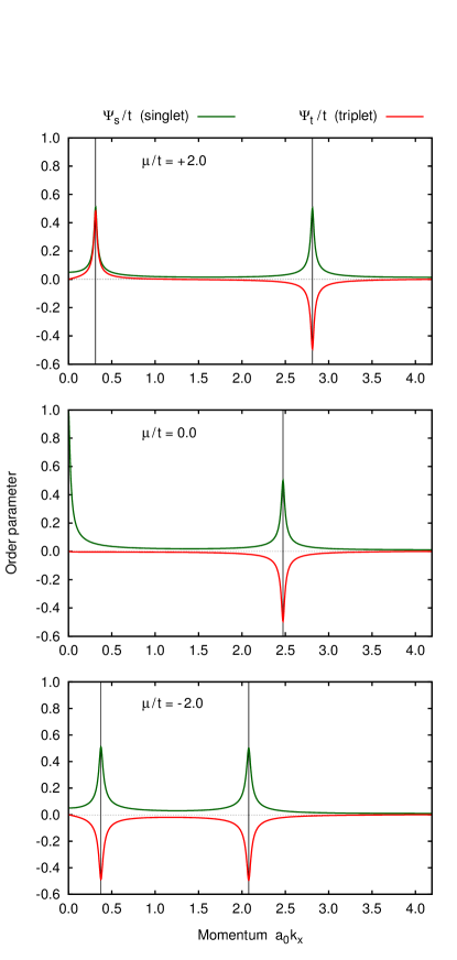
For small energies, i.e., in the vicinity of the band crossing, the dispersion of our tight-binding model is approximately described by the ideal Rashba model (14). Hence, near , the singlet and triplet amplitudes of the order parameter depend essentially only on the modulus . Figure 8 shows these amplitudes as a function of for three different values of the chemical potential (above, at, and below the band crossing), assuming a small value of the scalar gap parameter, .
We can understand these results qualitatively as follows: First, we restrict ourselves to momenta satisfying the condition (192). For small enough , we can then estimate using Eq. (218),
| (239) |
From Eqs. (237)–(238), we therefore obtain
| (240) |
This means, if is close to the Fermi line of the lower or upper band, then the singlet and triplet amplitudes are of equal magnitude and have the opposite or same sign, respectively. This is indeed clearly seen in Fig. 8. In particular, if the Fermi level is above the band crossing (), then there is one Fermi line for each band, and hence the ratio between and changes sign in the Brillouin zone as shown in the uppermost panel of Fig. 8.
IV.4 Gap equation and critical temperature
So far, we have calculated the gap function and the order parameter up to the scalar gap parameter . The latter was defined in Eq. (204), which can be written equivalently in terms of the order parameter and a trace over the spin indices as
| (241) |
Inserting our result for the order parameter, Eqs. (234)–(236), and using that
| (242) |
we obtain immediately
| (243) | ||||
| (244) |
which is equivalent to the scalar gap equation
| (245) |
Note that this equation agrees with the standard form of the gap equation in the SU(2)-symmetric case (see e.g. Ref. Vollhardt and Wölfle, 1990). The right-hand side depends on the gap parameter through the mean-field energies (see Eq. (218)). Equation (245) can be used to calculate
depending on the inverse temperature , the chemical potential and the coupling constant .
Before coming to the solution of Eq. (245) in the zero-temperature limit, we remark that the gap equation also allows to estimate the critical temperature , which is defined as the temperature where the gap vanishes.Vollhardt and Wölfle (1990) In the limit , we obtain from Eq. (245) the linearized gap equation
| (246) |
where are the eigenvalues of the free Hamiltonian. In terms of the total density of states (31), we can write this equation as
| (247) |
where we have re-introduced the stopping scale . Now, provided that is away from the band minimum, one may approximate the density of states by its value at the chemical potential, . The gap equation (247) then yields the standard estimate for the critical temperature 222See Eq. (3.48) in Ref. Vollhardt and Wölfle, 1990; the factor in the exponent of our Eq. (248) comes from the fact that refers to both bands of the model, and hence in the absence of the spin splitting would be twice the density of states defined in Ref. Vollhardt and Wölfle, 1990.
| (248) |
with . The parameter , which in pure mean-field studies is usually introduced by hand as a “cutoff energy” (sometimes identified with the Debye frequencyVollhardt and Wölfle (1990)), has in our approach a concrete meaning as the stopping scale of the RG flow.
IV.5 Solving the gap equation
In this subsection, we will solve the scalar gap equation (245) in the zero-temperature limit. We will first provide analytical expressions for the asymptotics of the solution, and then present our numerical solution for as a function of and . For , Eq. (245) reduces to
| (249) |
In terms of the density of states (31), we can write this equivalently as
| (250) |
We are most interested in the solution of the gap equation for , and in particular near the band minimum where the density of states diverges. For , the dispersion of the tight-binding model can be approximated by the ideal Rashba model (14), whose density of states is given by Eq. (33). By putting this into Eq. (250), we obtain
| (251) | ||||
Note that and are measured relative to the band crossing at , while the minimum of the lower band has the negative energy . For simplicity, we now ignore the integration boundaries depending on and instead integrate over the whole interval . Furthermore, as we are interested in the case where , we define the dimensionless variables
| (252) |
as well as the dimensionless coupling constant
| (253) |
In terms of these new variables, we can write the gap equation (251) more compactly as
| (254) |
We now analyze the asymptotics of the solution of this equation, focusing on two particular cases: and .
Case 1: . We substitute in Eq. (254)
| (255) |
Then, we can write the gap equation as
| (256) |
By our case assumptions, the prefactor on the right-hand side is small, i.e.,
| (257) |
Therefore, the integral in Eq. (256) must be large, which in turn is only possible if is small. We split the integral into two parts (using that ):
| (258) |
The first integral can be estimated as follows, using that and :
| (259) | ||||
where we have obtained the last result using Mathematica.Wolfram Research, Inc. (2015) In the second integral, we substitute :
| (260) | |||
| (261) |
This integral can in turn be split into two parts: one which is singular for ,
| (262) |
and one which approaches a constant value,
| (263) | ||||
This last integral has again been evaluated using Mathematica.Wolfram Research, Inc. (2015) Adding Eqs. (259), (262), and (263) yields
| (264) | ||||
The gap equation (256) can thus be approximated as
| (265) |
From this, we obtain the estimate
| (266) |
which is equivalent to
| (267) |
In particular, by our case assumption , we can verify a posteriori the condition which we have used in the derivation. Furthermore, by noting that the density of states, Eq. (33), can be written for as
| (268) |
we see that the result (267) is equivalent to
| (269) |
or in terms of the original parameters,
| (270) |
Note in particular the exponent, which coincides with the usual exponent in the SU(2) symmetric case.
Case 2: . This case corresponds to the situation where the chemical potential is precisely at the band minimum. We then obtain from Eq. (254),
| (271) |
By substituting , this is equivalent to
| (272) |
This integral has two contributions,
| (273) |
The first integral yields a constant,
| (274) |
which can be evaluated using MathematicaWolfram Research, Inc. (2015) as
| (275) |
The second integral can be estimated as follows, assuming that :
| (276) |
Combining Eqs. (274) and (276), we obtain
| (277) |
The gap equation (272) now reduces to
| (278) |
where the last estimate applies again for . Thus, we obtain
| (279) |
or in terms of the original parameters,
| (280) |
In particular, the condition is fulfilled for , which means that the above calculation (just as the discussion in Case 1) is only valid for sufficiently small coupling parameters.
![[Uncaptioned image]](/html/1409.7087/assets/x6.png)
![[Uncaptioned image]](/html/1409.7087/assets/x7.png)
For the numerical solution of Eq. (254), we have used the function fzero from GNU Octave.Eaton et al. (2014) We have fixed the coupling parameter to a small value, , and solved the implicit equation for the gap parameter . Figure 10 shows the resulting dependence of on the chemical potential . The characteristic features of the asymptotic solution are clearly reproduced in the numerical result: (i) the positive value of , (ii) the maximum of at small , and (iii) the exponential decay for large . Even quantitatively, there is a good agreement between the numerical data and the analytical results given by Eqs. (267) and (279). Finally, we have fixed the chemical potential to a tiny value () and plotted the dependence of the gap parameter on the coupling constant . The result is shown in Fig. 10. One clearly sees the quadratic dependence on , and the agreement with the analytical result (279) becomes perfect for small coupling constants.
V Conclusion
We have implemented a functional RG flow without SU(2) spin symmetry and used it to analyze the Rashba model with an attractive, local interaction. This model has a Hamiltonian whose kinetic term is not SU(2) spin invariant, while the interaction is invariant, and it is one of the simplest two-band correlated fermion models. Our RG flow results in an effective interaction slightly above the critical scale which is SU(2) invariant and attractive between singlet Cooper pairs of fermions with momenta and . We have applied mean-field theory to this interaction in order to calculate the gap function and the order parameter. The gap function is a pure singlet function, but the order parameter (defined as the expectation value of a Cooper pair field) has a nontrivial decomposition into singlet and triplet parts. While it is not surprising that an attractive interaction drives superconductivity, the symmetries of the gap function and the order parameter were not a priori obvious in the case without SU(2) symmetry. Besides these results, our analysis has also provided clarifications about more general theoretical issues, which we summarize and discuss further in the following.
The RG flow employed here does not require any a priori assumption on the type of symmetry breaking that may happen. Indeed, it is a standard level-two truncation of the fermionic RG equations in the symmetric phase. The fact that a local (hence in momentum space, constant) bare interaction gives rise to a singlet-pairing effective interaction at low scales, and that this interaction is with very high accuracy given by pairing, is thus a genuine result and not an input of our analysis. Besides the truncation, the projection to the Fermi lines performed here (as in most earlier studies) is the main approximation used. This approximation has been justified by power counting for the asymptotics of the flow of one-band models at low scales,Salmhofer and Honerkamp (2001); Metzner et al. (2012) but it is used more generally to make the RG equations amenable to numerics. In comparison to earlier definitions of this projection for multiband models, a crucial point of our work is a refined Fermi surface projection that makes no assumption on the relative importance of the contributions from different bands, and which is therefore compatible with the transformation between spin and band indices at all scales. It is this property that leads to the SU(2) invariance of the effective interaction. Our projection gives a flow in which at all scales, not only degrees of freedom near to the Fermi surface and in the conduction band, but also ones near to the Fermi surface and in higher bands (which have a propagator that is non-singular) contribute in an essential way to the flow.
This goes against the intuition in general discussions that “high-energy degrees of freedom, once integrated over, should no longer explicitly enter the RG equations at lower scales”, and one might even worry that some double counting was involved in our procedure. There is, however, no double counting problem here. Whether the above intuition is correct or not depends on the scheme and approximations that are used, and the projection simply has to match the properties of the scheme. In the one-line irreducible scheme that we use, the functional RG equations contain both a single-scale propagator and a full propagator . In the former, the energy must be close to the flowing scale, , but the latter contains only a condition that the energy is at least as big as the RG scale, . There is therefore no room for an additional assumption that all internal band indices save for the low-energy band are removed, and there is also no need for it since any such restriction is automatically enforced by the above-mentioned support properties of and . Conversely, momentum and band index configurations of the external variables that include upper bands may be driven nontrivially in the flow. Specifically, for the Cooper pair interaction, the condition and momentum conservation allow that such configurations couple to the singular flow in the particle-particle channel of the conduction band, i.e. to configurations and band indices such that , no matter whether is small. This is seen explicitly in our equations (167)–(169) for the subsystem of couplings , , , where , and the flow of , i.e. the coupling of the low-energy degrees of freedom, drags along all the other couplings, so that they all remain equally large at low scales if they are equal at the initial scale (as is the case for a local interaction). More generally, we have shown that our numerical solution of the RG equations is consistent with an analytical resummation of the particle-particle ladder. The latter provides a general explanation for the SU(2) symmetry of the effective interaction.
We remark that in other schemes, the RG equations are arranged differently. In the Polchinski scheme,Zanchi and Schulz (2000) there is indeed only a single-scale propagator on the right-hand side of the flow equation. However, in that hierarchy of equations, the flow for the four-point function is driven by the six-point function. It is well known that the analog of the level-two truncation in this scheme is to truncate the RG equation for the six-point function to the tree term with two four-point functions (see e.g. Ref. Zanchi and Schulz, 2000), but this introduces a scale integral over from to in the RG equation for the four-point function, and hence leads to a similar situation as above. In the Wick-ordered scheme,Salmhofer (1998); Halboth and Metzner (2000) all internal lines are indeed at or below the scale , so that a simpler projection scheme may suffice. The special kinematics of the Wick-ordered scheme has also been discussed in the treatment of the constrained random phase approximation (cRPA) and downfolding by functional RG methods.Honerkamp (2012)
Furthermore, our mean-field analysis has shown that one generally has to distinguish between the two different notions of a gap function and an order parameter. The reason why they are different lies in the Bogoliubov transformation: while the gap function can be deduced directly from the superconducting interaction, the order parameter requires the diagonalization of the mean-field Hamiltonian, Eq. (205), and therefore depends on the concrete form of its eigenvectors and eigenenergies. Unless the free Hamiltonian is diagonal (such that in Eq. (3)), the resulting order parameter will have a triplet contribution as given explicitly in Eq. (233). This result for the order parameter is not restricted to the particular model, but applies more generally to any time-reversal symmetric Hamiltonian of the form (1). Our formulas for the Bogoliubov transformation and the resulting order parameter therefore generalize the results of Ref. Sigrist and Ueda, 1991 to the case without SU(2) symmetry. Finally, by analytically and numerically solving the scalar gap equation for the Rashba model, we have shown that the gap size attains a constant value as the chemical potential approaches the minimum of the lower band. This constant value grows with the square of the strength of the superconducting interaction.
This work confirms the functional RG as a tool for investigating Fermi liquid instabilities in multiband and less symmetric systems, in particular in the absence of SU(2) symmetry. While we have applied it here to the case of the Rashba model with an attractive onsite interaction, our procedure can be generalized straightforwardly to investigate more complicated interactions such as spin-dependent nearest-neighbor or long-range interactions. Furthermore, it would be interesting to include a Zeeman term in the free Hamiltonian, which in Refs. Fujimoto, 2008; Sau et al., 2010; Alicea, 2010 is an ingredient for the predicted topological superconductivity. Combined with mean-field theory, the functional RG approach allows for an unambiguous prediction of the superconducting gap function and the order parameter. We expect this to be useful for an unbiased theoretical description of the low-temperature properties of correlated electron materials with spin-orbit coupling.
Acknowledgements.
This work was supported by the DFG Research Unit FOR 723. M. M. S. is supported by the Grant No. ERG-AdG-290623. We thank Ryotaro Arita, Mohammad S. Bahramy, Andreas Eberlein, Tilman Enss, Mario Fink, Lukas Janssen, Julian Lichtenstein, Titus Neupert, Christian Platt, Daniel D. Scherer, Ronald Starke, Ronny Thomale and Kambis Veschgini for discussions.Appendix A Tight-binding Rashba model
In this first appendix, we explain our conventions for the tight-binding description of electronic states on the hexagonal Bravais lattice in two dimensions. We derive the Rashba spin splitting from symmetry conditions, and subsequently construct a minimal tight-binding model which displays Rashba spin splitting near the center of the Brillouin zone. Furthermore, we derive the corresponding symmetry conditions for a two-particle interaction in a second-quantized framework.
A.1 Hexagonal Bravais lattice
All our formulas are valid in SI units.Bureau International des Poids et Mesures (2006) The hexagonal Bravais lattice in two dimensions (Ref. Levy, 1968, Table 2.2) is defined by
| (281) |
in terms of the primitive vectors
| (282) | ||||
| (283) |
where is the lattice constant. This Bravais lattice is also referred to as the direct lattice (or direct space). By contrast, the reciprocal lattice consists of all vectors with the property
| (284) |
It is given explicitly by
| (285) |
where the primitive vectors of the reciprocal lattice are defined by the condition ()
| (286) |
and given explicitly by
| (287) | ||||
| (288) |
The (first) Brillouin zone (also referred to as dual space or Bloch momentum space) is defined as the set of all points which lie closer to the origin than to any other reciprocal lattice vector. Defining for the set
| (289) |
which is the Brillouin zone shifted by the reciprocal lattice vector , we have for all the two properties
| (290) |
and
| (291) |
The hexagonal Bravais lattice and the corresponding Brillouin zone are shown in Figs. 12 and 12, respectively.
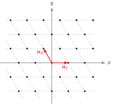
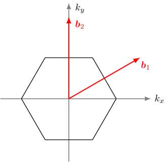
We consider a simple two-band model described by a non-interacting Hamiltonian acting on wave functions defined on the Bravais lattice. 333For the purposes of this article, we may take such a model Hamiltonian defined on the Bravais lattice as our starting point. On a more fundamental level, such a description should be derived from a fundamental Hamiltonian for the electrons in the periodic potential of the nuclei, which are assumed to be fixed at the sites of the Bravais lattice. This fundamental Hamiltonian acts on electronic wave functions defined on the continuous three-dimensional space (i.e., position space). For any lattice vector , the Hamiltonian matrix then corresponds to matrix elements of the fundamental Hamiltonian between two Wannier functions centered at lattice sites with distance vector . In a tight-binding description, one neglects these matrix elements if the distance exceeds a few lattice sites (see Ref. Essler et al., 2005, Chap. 1) In this model, any state vector can be characterized by its wave function in direct space or in dual space,
| (292) | ||||
| (293) |
Here, is a direct lattice vector, a spin index and a dual vector (or Bloch momentum). In the following (as in the main text) we also call a “momentum” (or “wave vector”), although strictly speaking momentum space refers to the continuous three-dimensional space . In particular, momentum space is related by Fourier transformation to position space (see footnote 93), just as the dual space is related to the direct space . The wave functions (292)–(293) are interrelated by Fourier transformation as follows:
| (294) | ||||
| (295) |
where
| (296) |
is the area of the Brillouin zone. In particular, the basis vectors in direct space and the basis vectors in dual space are given by their wave functions in direct space as
| (297) | ||||
| (298) |
The basis vectors in direct space are orthonormal,
| (299) |
and complete,
| (300) |
Note that Eq. (299) formally coincides with Eq. (297), although the interpretation is different. Similarly, the basis vectors in dual space are orthonormal and complete in the sense that
| (301) |
and
| (302) |
These properties can be derived using the identities
| (303) | ||||
| (304) |
Note that denotes the Kronecker delta,
| (305) |
whereas is the Dirac delta distribution which is normalized such that
| (306) |
In particular, since has the unit of an inverse area, the Dirac delta distribution in dual space has the unit of an area. The abbreviation (2) will be useful in the following to simplify expressions.
Next, we define the Hamiltonian matrices in direct and in dual space. For this purpose, let the translation operators , , be defined as linear operators acting on direct-space wave functions as
| (307) |
In particular, they act on the basis vectors in direct and respectively dual space as
| (308) | ||||
| (309) |
We assume that the Hamiltonian is invariant under all lattice translations, i.e.,
| (310) |
For the matrix elements of the Hamiltonian in direct space, this implies
| (311) | ||||
| (312) |
where is called the Hamiltonian matrix in direct space. On the other hand, in dual space we obtain
| (313) |
where the Hamiltonian matrix in dual space is related to the Hamiltonian matrix in direct space by
| (314) | ||||
| (315) |
These formulas are analogous to the Fourier transformation of wave functions, Eqs. (294)–(295).
Any complex matrix can be expanded in terms of the identity matrix and the Pauli matrices . In particular, we can write the Hamiltonian matrix in dual space, , as follows:
| (316) |
The Hermiticity of the Hamiltonian operator,
| (317) |
implies that the Hamiltonian matrix in dual space is also Hermitian, i.e.,
| (318) |
As a consequence, the functions , , , in Eq. (316) are real valued. In components, the representation (316) of the Hamiltonian matrix reads as
| (319) |
(where we have suppressed the dependencies). The Hamiltonian matrix in direct space, , can be expanded analogously as
| (320) |
However, Hermiticity implies that
| (321) |
hence and are not necessarily real (see Tables 4 and 4). The functions are related to by Fourier transformation analogous to Eqs. (314)–(315).
A.2 Symmetry conditions
| Possible symmetry | Transformation of basis functions | ||
|---|---|---|---|
| of the Hamiltonian | under the symmetry operation | ||
| Hermiticity | — | — | |
| Time-reversal | |||
| (Spatial inversion) | |||
| Three-fold rotation | |||
| Mirror reflection | |||
| Hamiltonian matrix | Pauli matrix representation | ||
|---|---|---|---|
| Hermiticity | |||
| Time-reversal | |||
| (Spatial inversion) | |||
| Three-fold rotation | |||
| Mirror reflection | |||
| Hamiltonian matrix | Pauli matrix representation | ||
|---|---|---|---|
| Hermiticity | |||
| Time-reversal | |||
| (Spatial inversion) | |||
| Three-fold rotation | |||
| Mirror reflection | |||
Besides the lattice translations, we consider the following symmetry operations which are defined by their action on direct-space wave functions (see Ref. Messiah, 1962):
-
(i)
Time-reversal:
(322) where “∗” denotes the complex conjugation.
-
(ii)
Spatial inversion:
(323) which leaves the spin invariant.
-
(iii)
Three-fold rotation:
(324) where the matrix acting on is given by
(325) If we identify the spin indices as , , such that formally,
(326) we can write Eq. (324) more compactly as
(327) -
(iv)
Mirror reflection:
(328) where acting on is defined as
(329) This matrix is self inverse, i.e., .
The above symmetry operations defined on the two-dimensional Bravais lattice are derived from their respective counterparts on the three-dimensional hexagonal lattice, , by the restriction to a single plane (i.e., to the lattice points with ). In particular, (iii) and (iv) correspond to the symmetries (rotation by around the axis) and (reflection in the vertical plane) of the three-dimensional point-group , which describes the Rashba semiconductor BiTeI.Ishizaka et al. (2011); Bahramy et al. (2011) The transformation properties of the basis functions (in direct and in dual space) under the symmetry operations (i)–(iv) are shown in Table 2.
We now assume that the Hamiltonian is Hermitian and invariant under the symmetries (i), (iii), and (iv). We shall, however, not assume that the Hamiltonian is invariant under spatial inversion (ii). In fact, the crystal structure of BiTeI lacks inversion symmetry, and this is one main reason—besides the large atomic spin-orbit coupling of the bismuth atoms—for the bulk Rashba spin splitting in this material (see Refs. Ishizaka et al., 2011, Bahramy et al., 2011, and the following discussion). The possible symmetries of the Hamiltonian operator (see Table 2) can be expressed equivalently in terms of the Hamiltonian matrix in direct or in dual space, or in terms of the functions and introduced in Appendix A.1. These symmetry conditions are shown in Table 4 (direct space) and in Table 4 (dual space), where we have included for the sake of completeness also the inversion symmetry.
In the following, we show that the symmetries (i), (iii) and (iv) already imply that near , the model is described by the Rashba Hamiltonian, Eq. (14): First, Hermiticity implies that and are real functions. By time-reversal symmetry, they satisfy (see Table 4)
| (330) | |||
| (331) |
(Note that inversion symmetry (ii) would imply , which combined with Eq. (331) yields . Hence, requiring time-reversal symmetry and inversion symmetry at the same time necessarily leads to a spin-degenerate band, which is indeed well known, see e.g. Ref. Dresselhaus et al., 2008, Sec. 16.4) The above equations (330)–(331) imply that is an even function, while are odd functions in the Bloch momentum . We can therefore expand them to quadratic order in as
| (332) | ||||
| (333) |
where , , and are real constants. Without loss of generality (by a constant energy shift), we may set . In matrix notation, Eqs. (332)–(333) can then be written as
| (334) |
and, respectively,
| (335) |
We go on to study the consequences of the three-fold rotation symmetry. By Table 4, this implies
| (336) | ||||
| (337) |
In the last equation, we have explicitly distinguished between the matrix acting on (which is the matrix given by Eq. (325)), and the matrix acting on , i.e.,
| (338) |
In terms of the matrices and , Eqs. (336)–(337) are equivalent to
| (339) | ||||
| (340) |
These conditions imply
| (341) | ||||
| (342) |
the analogous equations for , and furthermore,
| (343) |
Hence, the matrices and take the form
| (344) |
Finally, we consider the mirror reflection symmetry. From Table 4, we obtain the conditions
| (345) | ||||
| (346) |
where the matrix acting on is defined as
| (347) |
In terms of the matrices and , Eqs. (345)–(346) are equivalent to
| (348) | ||||
| (349) |
These conditions imply
| (350) |
and, respectively,
| (351) |
We are therefore left with only two parameters and , in terms of which the matrices and are completely determined as
| (352) |
By inserting these matrices into Eqs. (334)–(335) and using Eq. (316), we obtain the following Hamiltonian matrix up to quadratic order in :
| (353) | ||||
| (354) |
This coincides with the Rashba Hamiltonian (14) if we identify the parameters
| (355) |
Thus, we have shown that near , the Rashba Hamiltonian (14) can be derived from symmetry considerations only, by assuming time-reversal symmetry as well as three-fold rotation and mirror reflection symmetries.
A.3 Minimal tight-binding model
We now construct a minimal tight-binding model on the hexagonal Bravais lattice which is invariant under time-reversal, three-fold rotation, and mirror reflection symmetries (but not under inversion symmetry). By the argument of the preceding subsection, this model will necessarily be described near by the Rashba Hamiltonian. The minimal model will be defined in terms of the six nearest neighbor vectors (see Fig. 12)
| (356) | ||||
| (357) | ||||
| (358) | ||||
| (359) | ||||
| (360) | ||||
| (361) |
We assume that the Hamiltonian matrix in direct space (see Eq. (312)),
| (362) |
vanishes unless for some (this means, there is only “electron hopping” between nearest-neighbor sites). Consequently, the Hamiltonian matrix in direct space can be written as
| (363) |
In dual space, this implies by Fourier transformation (see Eq. (314))
| (364) |
The expansions (363)–(364) hold analogously for the functions and defined in Sec. A.1. We now employ the constraints imposed on these functions by the Hermiticity as well as the time-reversal, three-fold rotation, and mirror reflection symmetries. The function has to be real and satisfy (see Table 4)
| (365) | ||||
| (366) | ||||
| (367) |
Hence, if is restricted to nearest-neighbor vectors, it is completely determined by only one real parameter,
| (368) |
By Eqs. (365)–(367), we then have
| (369) |
Therefore, is given in direct space by
| (370) |
and in dual space by
| (371) | |||
| (372) |
In terms of the dimensionless quantity , this can be written equivalently as
| (373) | ||||
where we have used Eqs. (356)–(361). Similarly, the function has to be purely imaginary and satisfy
| (374) | ||||
| (375) | ||||
| (376) |
In particular, using that , we find
| (377) | ||||
| (378) | ||||
| (379) |
and consequently, by Eq. (347),
| (380) |
By restricting to nearest-neighbor vectors, it is therefore completely determined by two real parameters , which we define as
| (381) |
Thus, is given in direct space by
| (382) | ||||
| (383) |
where we have abbreviated
| (384) |
In components, this is equivalent to
| (393) | ||||
| (394) |
or by Fourier transformation,
| (403) | ||||
| (404) |
With defined in Eq. (4), we obtain the following explicit expressions:
| (405) | ||||
| (406) | ||||
| (407) |
In summary, the minimal tight-binding model is defined in dual space by Eq. (316), where the functions and are expressed in terms of the real “hopping” parameters , , and by Eqs. (373) and (405)–(407).
For small wave vectors, more precisely for
| (408) |
we can expand the functions and around . By approximating
| (409) |
we obtain from Eqs. (373) and (405)–(407) the following expressions, which are valid to second order in the momentum:
| (410) |
and
| (411) | ||||
| (412) | ||||
| (413) |
Note that the parameter does not appear at all in this second-order expansion. For the Hamiltonian matrix, we thus obtain
| (414) |
where we have neglected the constant energy shift in Eq. (410). As expected, the above expression coincides again with the Rashba Hamiltonian (14) if we identify the parameters
| (415) |
Note that in the main text, we have set the model parameter to zero such that vanishes identically (not only to second order in the momentum). The formulas (373) and (405)–(407) then coincide with Eqs. (5)–(8) in the main text.
A.4 Second quantization
In the previous subsection, we have defined the Hamiltonian of a minimal tight-binding model by specifying its matrix elements in direct space,
| (416) |
The (first-quantized) Hamiltonian can thus be written as
| (417) |
By Fourier transformation, we obtain the corresponding representation in dual space,
| (418) |
Under second quantization, the Hamiltonian turns into (see e.g. Ref. Giuliani and Vignale, 2005)
| (419) |
or equivalently,
| (420) |
The second-quantized Hamiltonian is defined as a Hermitian operator by its action on fermionic -particle states,
| (421) | ||||
The operators
| (422) | ||||
| (423) |
annihilate and create, respectively, a basis vector with direct lattice vector and spin . Similarly, the operators
| (424) | ||||
| (425) |
annihilate and create, respectively, a basis vector with Bloch momentum and spin . Note that for any single-particle state , the annihilation operator is defined by its action on fermionic -particle states as
| (426) | ||||
where the notation in the last line means that the vector is omitted from the antisymmetrized product. The corresponding creation operator is defined by
| (427) | ||||
In particular, the maps
| (428) | ||||
| (429) |
are antilinear and linear respectively in the sense that
| (430) | ||||
| (431) |
As the notation suggests, the creator is the Hermitian adjoint of the annihilator . The operators (422)–(423) in direct space are related to their counterparts (424)–(425) in dual space by
| (432) | ||||
| (433) |
which can be shown using the relation
| (434) |
| Annihilation operator | Creation operator | |
|---|---|---|
| Time-reversal | ||
| (Spatial inversion) | ||
| Three-fold rotation | ||
| Mirror reflection |
| Interaction | Interaction kernel | |
|---|---|---|
| operator | in dual space (see Eq. (443)) | |
| Hermiticity | ||
| Time-reversal | ||
| (Spatial inversion) | ||
| Three-fold rotation | ||
| Mirror reflection | ||
Under symmetries, the annihilation and creation operators transform as
| (435) |
where , or . In this equation, denotes the second-quantized symmetry operator, which is defined as an (anti)unitary operator by its action on fermionic -particle states,
| (436) |
Its inverse is given by
| (437) |
Using Eq. (435) and the transformation laws for the basis vectors shown in Table 2, one can deduce the explicit transformation laws for the operators and as shown in Table 6. Using these transformation laws and the symmetries of the Hamiltonian matrix in dual space (Table 4), one recovers again the symmetries of the second-quantized Hamiltonian (420), i.e.,
| (438) |
for or . In the following (as in the main text), we will suppress the operation of second quantization in the notation and simply write, for example, . The distinction between first- and second-quantized operators should, however, always be clear from the context.
In addition to the quadratic Hamiltonian (420), we consider a quartic (two-particle) interaction of the form
| (439) | ||||
(note the order of the annihilation operators). We assume that is translation invariant just as the free Hamiltonian (see Sec. A.1), i.e.,
| (440) |
This implies that
| (441) | ||||
or in dual space,
| (442) | ||||
Note that in the last line, we formally sum over all reciprocal lattice vectors . The condition that all momenta lie in the first Brillouin zone, however, fixes precisely one vector which contributes to the sum. Hence, the translation-invariant interaction term (439) can be written in dual space as
| (443) | ||||
This formula corresponds to Eq. (II) in the main text.
Without loss of generality, we may assume that the interaction kernel is antisymmetric with respect to its first two and its last two arguments, i.e.,
| (444) | |||
| (445) |
Furthermore, we assume that is Hermitian and invariant under time-reversal, three-fold rotation, and mirror reflection symmetries. These conditions on the operator translate again—using the transformation properties of the creation and annihilation operators shown in Table 6—into conditions on the interaction kernel, which are shown in Table 6. (For the sake of completeness,
Appendix B Statistical field theory
In this second appendix, we fix our conventions for the temperature Green functions, in terms of which the renormalization group equations have been formulated in the main text. For the non-expert in statistical field theory, we also provide a brief summary of the most important definitions and properties of temperature Green functions.
B.1 Temperature Green functions
For defining the temperature Green functions of our second-quantized tight-binding model, let
| (446) |
where denotes the full Hamiltonian of the interacting many-fermion system (given by Eqs. (420) and (443); in Appendix A, was denoted by for simplicity). Furthermore, denotes the chemical potential and the particle-number operator, which is given in terms of the annihilation and creation operators of Sec. A.4 by
| (447) |
In terms of these operators, the grand canonical partition function can be written as
| (448) |
where is the inverse temperature. Furthermore, for any operator and for we define
| (449) |
which is analogous to the time evolution in the Heisenberg picture if we identify . Therefore, is called “imaginary time.” For and for , the -point temperature Green function (or imaginary-time Green function) is defined as
| (450) | ||||
Here, the time-ordering operator is defined with respect to the imaginary-time arguments. Thus, for any operators , the time-ordered product is given by
| (451) | ||||
In this formula, denotes the symmetric group of elements, i.e., the group of all permutations of the set , and denotes the character of the permutation . Furthermore, is the Heaviside step function defined by
| (452) |
Note that the Green functions defined by Eq. (450) are dimensionless. In the following, we list the most important properties of the temperature Green functions (for details, see the standard references Fetter and Walecka, 1971; Zinn-Justin, 1996; Negele and Orland, 1998; Salmhofer, 1999).
(i) Antiperiodicity. The temperature Green functions satisfy antiperiodic boundary conditions in the following sense: for each , the values of at and are related by
| (453) | ||||
Therefore, the temperature Green functions—which were originally defined only for by Eq. (450)—can be continued to antiperiodic functions of .
(ii) Fourier transformation. The Fourier transforms of the temperature Green functions are defined by
| (454) | |||
or conversely,
| (455) | |||
Here, are fermionic Matsubara frequencies due to the antiperiodicity (property (i)) of the temperature Green functions. By our conventions, the Fourier transform of any function has the same dimension as the function itself. In particular, the temperature Green functions in the direct space/time domain and in the dual space/frequency domain are all dimensionless.
(iii) Translation invariance. The temperature Green functions are always translation invariant with respect to the imaginary-time arguments. If the Hamiltonian is invariant with respect to spatial translations, then the same also applies to the Green functions. In particular, the two-point Green function can then be written as
| (456) |
or equivalently, by Fourier transformation,
| (457) | ||||
Similarly, the four-point Green function can be written in the Fourier domain as
| (458) | |||
where the reciprocal lattice vector is fixed by the condition that all momenta lie in the first Brillouin zone.
(iv) Symmetries. The Green functions defined by Eq. (450) inherit the symmetries of the Hamiltonian (446). In particular, the two-point Green function
| (459) |
(defined as the Fourier transform of Eq. (456) with respect to the spatial variables) transforms under symmetries in the same way as the free Hamiltonian matrix (see Table 4). Moreover, the four-point Green function in the Bloch momentum/time domain
| (460) |
transforms under symmetries in the same way as the interaction kernel (see Table 6). In the frequency domain, time reversal also changes the sign of the Matsubara frequencies, i.e., time-reversal symmetry is expressed by
| (461) | ||||
and similar conditions on the higher -point Green functions. All other symmetry operations act only on the spatial variables and hence leave the frequency arguments unchanged.
(v) Feynman graph expansion. The temperature Green functions have a perturbative expansion in terms of the interaction kernel and the free two-point Green function (also called the non-interacting Green function or covariance), which is defined as
| (462) | ||||
with and
| (463) |
Concretely, the th-order contribution to the -point Green function is given by the sum of all bubble-free Feynman graphs with interaction vertices and external legs. Here, bubble-free means that every interaction vertex is connected (through a series of free Green function lines and interaction vertices) to at least one external point.
B.2 Grassmann field integral
The Grassmann field integral (also called functional integral, or path integral) is useful for organizing the Feynman graph expansion of the fermionic temperature Green functions in an efficient way. We consider the Grassmann algebra generated by the elements (called Grassmann fields)
| (464) |
where is a multi-index containing the lattice site , the spin variable , and the imaginary-time variable . We impose antiperiodic boundary conditions,
| (465) | ||||
| (466) |
Furthermore, we consider the Grassmann algebra of the source fields
| (467) |
which satisfy the same boundary conditions (465)–(466), and which also anticommute with the fields . The Green function generator is an element of defined by
| (468) |
with the normalization constant
| (469) |
In these equations, is the inverse of the free two-point Green function (462). Furthermore,
| (470) |
where the integration over multi-indices is defined as in Eq. (71). Moreover, we have defined
| (471) | |||
In terms of the interaction kernel (63), this can be written equivalently as
| (472) | ||||
Now, the partition function (448) coincides with the field-independent term of the Green function generator (468),
| (473) |
and the temperature Green functions can be represented as Grassmann derivatives of with respect to the source fields: for ,
| (474) |
This important formula provides the connection between the operator formalism and the path integral formalism of statistical field theory.
B.3 Connected Green functions
The connected Green function generator is defined as another element of the Grassmann algebra of the source fields. It is the natural logarithm of the Green function generator divided by the field-independent term,
| (475) |
For , the connected temperature Green functions are defined as the Grassmann derivatives of :
| (476) | ||||
The connected Green functions have the same properties (i)–(iv) as the ordinary Green functions. They also have a Feynman graph expansion in terms of the interaction kernel and the free two-point Green function: the th-order contribution to the connected -point Green function is given by the sum of all connected Feynman graphs with interaction vertices and external legs. Here, connected means that every interaction vertex is connected (through a series of free Green function lines and interaction vertices) to every external point. The connected Green functions are related to the ordinary Green functions by the following equations: for ,
| (477) |
for ,
| (478) | |||
and similar equations for the higher -point Green functions (see e.g. Ref. Zinn-Justin, 1996).
B.4 One-line irreducible Green functions
| |
The one-line irreducible Green function generator is defined as the Legendre transform of the connected Green function generator , i.e.,
| (479) |
where the new source fields are defined by
| (480) |
We assume that these new source fields again generate the Grassmann algebra . For , the one-line irreducible temperature Green functions are defined by
| (481) | ||||
The one-line irreducible Green functions have again the same properties (i)–(iv) as the ordinary Green functions. In perturbation theory, is represented as
| (482) |
where is the free two-point Green function and the self-energy. The th-order contribution to the self-energy is given by the sum of all amputated, one-line irreducible Feynman graphs with interaction vertices and two external legs. Here, amputated means that all external Green function lines (i.e., the free two-point Green functions with external arguments) are removed; one-line irreducible means that by removing any single internal Green function line, the remaining Feynman graph is still connected. Similarly, for , equals times the sum of all amputated, one-line irreducible Feynman graphs with external legs. In particular, the two first-order Feynman graphs contributing to are shown in Table 7. The one-line irreducible Green functions are related to the connected Green functions by the following equations: for ,
| (483) |
for ,
| (484) | |||
and similar equations for (see Refs. Veschgini and Salmhofer, 2013; Negele and Orland, 1998). Of particular interest is the one-line irreducible four-point Green function , which is commonly interpreted as an “effective two-body interaction between two particles propagating in a many-particle medium” (Ref. Negele and Orland, 1998, p. 118; see also Ref. Nozières, 1997, Chap. 6).
Appendix C Projected RG equations
In this last appendix, we derive the RG equations (109)–(112) for the projected interaction vertex, and we show how the mean-field interaction (121) is deduced from our numerical result for the projected vertex.
C.1 Derivation
For deriving the RG equations (109)–(112), we put our refined projection ansatz (103) into Eqs. (86)–(89). Note that in (87)–(89), we have used the antisymmetry of the interaction vertex in its last two arguments to move the momentum into the last argument of , which is then fixed by momentum conservation, . This way of writing the RG equations will prove useful in the following, because it avoids ambiguities in the projection of on a representative momentum. First, consider the loop terms given by Eq. (90). We can write them equivalently as
| (485) |
with the functions given by Eqs. (91)–(92). Using the symmetry of under the exchange of its two arguments, we can also rewrite Eq. (485) as
| (486) |
We now evaluate Eq. (86) at the representative momenta,
| (487) |
and put the ansatz (103) into the right-hand side of this equation. We consider separately the particle-particle, crossed particle-hole, and direct particle-hole terms given, respectively, by Eqs. (87)–(89).
(i) Particle-particle term. From Eq. (87), we obtain
| (488) | ||||
In the second term in square brackets, we relabel the integration and summation variables
| (489) |
This leads to the equivalent expression
| (490) | ||||
Here we have used that
| (491) |
By performing the integral over and changing the order of the summations and integrations, we obtain
| (492) | |||
We now employ the following approximation: for ,
| (493) |
Then, Eq. (492) can be further simplified to
| (494) | ||||
where we have defined
| (495) | ||||
These equations are identical to Eqs. (110) and (113) in the main text.
(ii) Particle-hole terms. Next, we obtain from Eq. (88),
| (496) | |||
In the second term in square brackets, we relabel again
| (497) |
and use that
| (498) |
Performing the same steps as for the particle-particle term, we arrive at Eq. (111). Finally, Eq. (89) obviously implies Eq. (112), and this completes the derivation.
C.2 Mean-field interaction
We now show explicitly how the interaction (121) is deduced from our numerical result (120) for the projected interaction vertex. By putting Eq. (120) into the projection ansatz (103), we obtain the following interaction operator (analogous to Eq. (II) for the initial interaction),
| (499) | ||||
We now evaluate the sums over patch indices and the integral over for each fixed and : First, the indices and are uniquely determined by the characteristic functions
| (500) |
The index is subsequently fixed by the function
| (501) |
Finally, the integral over is restricted by the function
| (502) |
to the patch . We can therefore approximate
| (503) |
and similarly,
| (504) |
The integrand then depends on only through the characteristic function (502), and we can evaluate the integral as
| (505) |
Here, is the area of the Brillouin zone, whereas is the area of the patch . We assume that all patches are of comparable size, such that
| (506) |
with the number of patches. Thus we obtain from Eq. (499),
| (507) |
which coincides with Eq. (121) in the main text.
References
- Sinova and Žutić (2012) J. Sinova and I. Žutić, Nat. Mater. 11, 368 (2012).
- Barnes et al. (2014) S. E. Barnes, J. Ieda, and S. Maekawa, Sci. Rep. 4, 4105 (2014).
- Rashba (1960) E. I. Rashba, Sov. Phys.–Solid State 2, 1109 (1960), Fiz. Tverd. Tela 2, 1224 (1960).
- Nitta et al. (1997) J. Nitta, T. Akazaki, H. Takayanagi, and T. Enoki, Phys. Rev. Lett. 78, 1335 (1997).
- LaShell et al. (1996) S. LaShell, B. A. McDougall, and E. Jensen, Phys. Rev. Lett. 77, 3419 (1996).
- Hoesch et al. (2004) M. Hoesch, M. Muntwiler, V. N. Petrov, M. Hengsberger, L. Patthey, M. Shi, M. Falub, T. Greber, and J. Osterwalder, Phys. Rev. B 69, 241401 (2004).
- Pacilé et al. (2006) D. Pacilé, C. R. Ast, M. Papagno, C. Da Silva, L. Moreschini, M. Falub, A. P. Seitsonen, and M. Grioni, Phys. Rev. B 73, 245429 (2006).
- Ast et al. (2007a) C. R. Ast, J. Henk, A. Ernst, L. Moreschini, M. C. Falub, D. Pacilé, P. Bruno, K. Kern, and M. Grioni, Phys. Rev. Lett. 98, 186807 (2007a).
- Ast et al. (2007b) C. R. Ast, G. Wittich, P. Wahl, R. Vogelgesang, D. Pacilé, M. C. Falub, L. Moreschini, M. Papagno, M. Grioni, and K. Kern, Phys. Rev. B 75, 201401 (2007b).
- Ishizaka et al. (2011) K. Ishizaka, M. S. Bahramy, H. Murakawa, M. Sakano, T. Shimojima, T. Sonobe, K. Koizumi, S. Shin, H. Miyahara, A. Kimura, et al., Nat. Mater. 10, 521 (2011).
- Bahramy et al. (2011) M. S. Bahramy, R. Arita, and N. Nagaosa, Phys. Rev. B 84, 041202 (2011).
- Schober et al. (2012) G. A. H. Schober, H. Murakawa, M. S. Bahramy, R. Arita, Y. Kaneko, Y. Tokura, and N. Nagaosa, Phys. Rev. Lett. 108, 247208 (2012).
- Eremeev et al. (2012) S. V. Eremeev, I. A. Nechaev, Y. M. Koroteev, P. M. Echenique, and E. V. Chulkov, Phys. Rev. Lett. 108, 246802 (2012).
- Eremeev et al. (2013) S. V. Eremeev, I. P. Rusinov, I. A. Nechaev, and E. V. Chulkov, New J. Phys. 15, 075015 (2013).
- Rashba (2012) E. I. Rashba, Phys. Rev. B 86, 125319 (2012).
- Datta and Das (1990) S. Datta and B. Das, Appl. Phys. Lett. 56, 665 (1990).
- Sinova et al. (2004) J. Sinova, D. Culcer, Q. Niu, N. A. Sinitsyn, T. Jungwirth, and A. H. MacDonald, Phys. Rev. Lett. 92, 126603 (2004).
- Miron et al. (2010) I. M. Miron, G. Gaudin, S. Auffret, B. Rodmacq, A. Schuhl, S. Pizzini, J. Vogel, and P. Gambardella, Nat. Mater. 9, 230 (2010).
- Wunderlich et al. (2010) J. Wunderlich, B.-G. Park, A. C. Irvine, L. P. Zârbo, E. Rozkotová, P. Nemec, V. Novác, J. Sinova, and T. Jungwirth, Science 330, 1801 (2010).
- Jungwirth et al. (2012) T. Jungwirth, J. Wunderlich, and K. Olejník, Nat. Mater. 11, 382 (2012).
- Édel’shteǐn (1989) V. M. Édel’shteǐn, Sov. Phys.–JETP 68, 1244 (1989), ZhETF 95, 2151 (1989).
- Gor’kov and Rashba (2001) L. P. Gor’kov and E. I. Rashba, Phys. Rev. Lett. 87, 037004 (2001).
- Frigeri et al. (2004) P. A. Frigeri, D. F. Agterberg, A. Koga, and M. Sigrist, Phys. Rev. Lett. 92, 097001 (2004).
- Sigrist and Mineev (2012) M. Sigrist and V. Mineev, in Non-centrosymmetric superconductors. Introduction and overview, Lecture Notes in Physics, Vol. 847, edited by E. Bauer and M. Sigrist (Springer-Verlag, Berlin/Heidelberg, 2012) pp. 129–154.
- Fujimoto (2008) S. Fujimoto, Phys. Rev. B 77, 220501 (2008).
- Sau et al. (2010) J. D. Sau, R. M. Lutchyn, S. Tewari, and S. Das Sarma, Phys. Rev. Lett. 104, 040502 (2010).
- Alicea (2010) J. Alicea, Phys. Rev. B 81, 125318 (2010).
- Beenakker (2013) C. Beenakker, Annu. Rev. Condens. Matter Phys. 4, 113 (2013).
- Lutchyn et al. (2010) R. M. Lutchyn, J. D. Sau, and S. Das Sarma, Phys. Rev. Lett. 105, 077001 (2010).
- Oreg et al. (2010) Y. Oreg, G. Refael, and F. von Oppen, Phys. Rev. Lett. 105, 177002 (2010).
- Mourik et al. (2012) V. Mourik, K. Zuo, S. M. Frolov, S. R. Plissard, E. P. A. M. Bakkers, and L. P. Kouwenhoven, Science 336, 1003 (2012).
- Williams et al. (2012) J. R. Williams, A. J. Bestwick, P. Gallagher, S. S. Hong, Y. Cui, A. S. Bleich, J. G. Analytis, I. R. Fisher, and D. Goldhaber-Gordon, Phys. Rev. Lett. 109, 056803 (2012).
- Santos et al. (2010) L. Santos, T. Neupert, C. Chamon, and C. Mudry, Phys. Rev. B 81, 184502 (2010).
- Bardeen et al. (1957) J. Bardeen, L. N. Cooper, and J. R. Schrieffer, Phys. Rev. 108, 1175 (1957).
- Thouless (1960) D. J. Thouless, Ann. Phys. (Amsterdam, Neth.) 10, 553 (1960).
- Salmhofer and Honerkamp (2001) M. Salmhofer and C. Honerkamp, Prog. Theor. Phys. 105, 1 (2001).
- Cooper (1956) L. N. Cooper, Phys. Rev. 104, 1189 (1956).
- Kohn and Luttinger (1965) W. Kohn and J. M. Luttinger, Phys. Rev. Lett. 15, 524 (1965).
- Feldman et al. (1997) J. Feldman, H. Knörrer, R. Sinclair, and E. Trubowitz, Helv. Phys. Acta 70, 154 (1997).
- Sinclair (1996) R. M. Sinclair, Computational evidence for superconductivity in a repulsive model, Ph.D. thesis, ETH Zürich (1996).
- Vafek and Wang (2011) O. Vafek and L. Wang, Phys. Rev. B 84, 172501 (2011).
- Wang and Vafek (2014) L. Wang and O. Vafek, Physica C 497, 6 (2014).
- Metzner et al. (2012) W. Metzner, M. Salmhofer, C. Honerkamp, V. Meden, and K. Schönhammer, Rev. Mod. Phys. 84, 299 (2012).
- Honerkamp et al. (2001) C. Honerkamp, M. Salmhofer, N. Furukawa, and T. M. Rice, Phys. Rev. B 63, 035109 (2001).
- Honerkamp and Salmhofer (2001) C. Honerkamp and M. Salmhofer, Phys. Rev. Lett. 87, 187004 (2001).
- Husemann et al. (2012) C. Husemann, K.-U. Giering, and M. Salmhofer, Phys. Rev. B 85, 075121 (2012).
- Giering and Salmhofer (2012) K.-U. Giering and M. Salmhofer, Phys. Rev. B 86, 245122 (2012).
- Eberlein and Metzner (2014) A. Eberlein and W. Metzner, Phys. Rev. B 89, 035126 (2014).
- Eberlein (2014) A. Eberlein, Phys. Rev. B 90, 115125 (2014).
- Wang et al. (2009) F. Wang, H. Zhai, Y. Ran, A. Vishwanath, and D.-H. Lee, Phys. Rev. Lett. 102, 047005 (2009).
- Platt et al. (2009) C. Platt, C. Honerkamp, and W. Hanke, New J. Phys. 11, 055058 (2009).
- Thomale et al. (2009) R. Thomale, C. Platt, J. Hu, C. Honerkamp, and B. A. Bernevig, Phys. Rev. B 80, 180505 (2009).
- Thomale et al. (2011) R. Thomale, C. Platt, W. Hanke, and B. A. Bernevig, Phys. Rev. Lett. 106, 187003 (2011).
- Platt et al. (2011) C. Platt, R. Thomale, and W. Hanke, Phys. Rev. B 84, 235121 (2011).
- Platt et al. (2012) C. Platt, R. Thomale, C. Honerkamp, S.-C. Zhang, and W. Hanke, Phys. Rev. B 85, 180502 (2012).
- Lichtenstein et al. (2014) J. Lichtenstein, S. A. Maier, C. Honerkamp, C. Platt, R. Thomale, O. K. Andersen, and L. Boeri, Phys. Rev. B 89, 214514 (2014).
- Wang et al. (2013) Q. H. Wang, C. Platt, Y. Yang, C. Honerkamp, F. C. Zhang, W. Hanke, T. M. Rice, and R. Thomale, EPL 104, 17013 (2013).
- Honerkamp (2008) C. Honerkamp, Phys. Rev. Lett. 100, 146404 (2008).
- Kiesel et al. (2012) M. L. Kiesel, C. Platt, W. Hanke, D. A. Abanin, and R. Thomale, Phys. Rev. B 86, 020507 (2012).
- Wu et al. (2013) W. Wu, M. M. Scherer, C. Honerkamp, and K. Le Hur, Phys. Rev. B 87, 094521 (2013).
- Janssen and Herbut (2014) L. Janssen and I. F. Herbut, Phys. Rev. B 89, 205403 (2014).
- Classen et al. (2014) L. Classen, M. M. Scherer, and C. Honerkamp, Phys. Rev. B 90, 035122 (2014).
- Classen et al. (2015) L. Classen, I. F. Herbut, L. Janssen, and M. M. Scherer, Phys. Rev. B 92, 035429 (2015).
- Scherer et al. (2012a) M. M. Scherer, S. Uebelacker, and C. Honerkamp, Phys. Rev. B 85, 235408 (2012a).
- Lang et al. (2012) T. C. Lang, Z. Y. Meng, M. M. Scherer, S. Uebelacker, F. F. Assaad, A. Muramatsu, C. Honerkamp, and S. Wessel, Phys. Rev. Lett. 109, 126402 (2012).
- de la Peña et al. (2014) D. S. de la Peña, M. M. Scherer, and C. Honerkamp, Ann. Phys. (Berlin, Ger.) 526, 366 (2014).
- Scherer et al. (2012b) M. M. Scherer, S. Uebelacker, D. D. Scherer, and C. Honerkamp, Phys. Rev. B 86, 155415 (2012b).
- Platt et al. (2013) C. Platt, W. Hanke, and R. Thomale, Adv. Phys. 62, 453 (2013).
- Maier et al. (2014) S. A. Maier, A. Eberlein, and C. Honerkamp, Phys. Rev. B 90, 035140 (2014).
- Scherer et al. (2014) D. D. Scherer, M. M. Scherer, G. Khaliullin, C. Honerkamp, and B. Rosenow, Phys. Rev. B 90, 045135 (2014).
- Sigrist and Ueda (1991) M. Sigrist and K. Ueda, Rev. Mod. Phys. 63, 239 (1991).
- Wang et al. (2014) J. Wang, A. Eberlein, and W. Metzner, Phys. Rev. B 89, 121116 (2014).
- Reiss et al. (2007) J. Reiss, D. Rohe, and W. Metzner, Phys. Rev. B 75, 075110 (2007).
- Boiko and Rashba (1960) I. I. Boiko and E. I. Rashba, Sov. Phys.–Solid State 2, 1692 (1960), Fiz. Tverd. Tela 2, 1874 (1960).
- Winkler (2003) R. Winkler, Spin-orbit coupling effects in two-dimensional electron and hole systems (Springer-Verlag, Berlin/Heidelberg, 2003).
- Salmhofer et al. (2004) M. Salmhofer, C. Honerkamp, W. Metzner, and O. Lauscher, Prog. Theor. Phys. 112, 943 (2004).
- Gersch et al. (2005) R. Gersch, C. Honerkamp, D. Rohe, and W. Metzner, Eur. Phys. J. B 48, 349 (2005).
- Note (1) Note the prefactor in Eq. (62\@@italiccorr): The factor 2 comes from the fact that there are indeed two first-order Feynman graphs contributing to (see Table 7), while appears as a prefactor of every -th order Feynman graph. In particular, both sides of Eq. (62\@@italiccorr) have the same dimension, because by our conventions the interaction kernel has the dimension of an energy, whereas all Green functions are dimensionless (see Appendix B).
- Starke and Kresse (2012) R. Starke and G. Kresse, Phys. Rev. B 85, 075119 (2012).
- Salmhofer (1999) M. Salmhofer, Renormalization. An introduction (Sprin-ger-Verlag, Berlin/Heidelberg, 1999).
- Honerkamp and Salmhofer (2003) C. Honerkamp and M. Salmhofer, Phys. Rev. B 67, 174504 (2003).
- Salmhofer (1998) M. Salmhofer, Commun. Math. Phys. 194, 249 (1998).
- Halboth and Metzner (2000) C. J. Halboth and W. Metzner, Phys. Rev. Lett. 85, 5162 (2000).
- Mineev and Samokhin (1999) V. P. Mineev and K. V. Samokhin, Introduction to unconventional superconductivity (Gordon and Breach Science Publishers, Amsterdam, 1999).
- Vollhardt and Wölfle (1990) D. Vollhardt and P. Wölfle, The superfluid phases of Helium 3 (Taylor & Francis, London, 1990).
- Note (2) See Eq. (3.48) in Ref. \rev@citealpnumVollhardt; the factor in the exponent of our Eq. (248\@@italiccorr) comes from the fact that refers to both bands of the model, and hence in the absence of the spin splitting would be twice the density of states defined in Ref. \rev@citealpnumVollhardt.
- Wolfram Research, Inc. (2015) Wolfram Research, Inc., Mathematica, Version 10.3 (Champaign, IL, 2015).
- Eaton et al. (2014) J. W. Eaton, D. Bateman, S. Hauberg, and R. Wehbring, GNU Octave version 3.8.1 manual: a high-level interactive language for numerical computations (CreateSpace Independent Publishing Platform, 2014).
- Zanchi and Schulz (2000) D. Zanchi and H. J. Schulz, Phys. Rev. B 61, 13609 (2000).
- Honerkamp (2012) C. Honerkamp, Phys. Rev. B 85, 195129 (2012).
- Bureau International des Poids et Mesures (2006) Bureau International des Poids et Mesures, A concise summary of the international system of units, the SI (2006).
- Levy (1968) R. A. Levy, Principles of solid state physics (Academic Press, New York/London, 1968).
- Note (3) For the purposes of this article, we may take such a model Hamiltonian defined on the Bravais lattice as our starting point. On a more fundamental level, such a description should be derived from a fundamental Hamiltonian for the electrons in the periodic potential of the nuclei, which are assumed to be fixed at the sites of the Bravais lattice. This fundamental Hamiltonian acts on electronic wave functions defined on the continuous three-dimensional space (i.e., position space). For any lattice vector , the Hamiltonian matrix then corresponds to matrix elements of the fundamental Hamiltonian between two Wannier functions centered at lattice sites with distance vector . In a tight-binding description, one neglects these matrix elements if the distance exceeds a few lattice sites (see Ref. \rev@citealpnum[Chap. 1]Hubbard).
- Messiah (1962) A. Messiah, Quantum mechanics, Vol. 2 (North Holland Publishing Company, Amsterdam, 1962).
- Dresselhaus et al. (2008) M. S. Dresselhaus, G. Dresselhaus, and A. Jorio, Group theory. Application to the physics of condensed matter (Springer-Verlag, Berlin/Heidelberg, 2008).
- Giuliani and Vignale (2005) G. F. Giuliani and G. Vignale, Quantum theory of the electron liquid (Cambridge University Press, 2005).
- Fetter and Walecka (1971) A. L. Fetter and J. D. Walecka, Quantum theory of many-particle systems (McGraw-Hill, San Francisco, 1971).
- Zinn-Justin (1996) J. Zinn-Justin, Quantum field theory and critical phenomena, 3rd ed. (Clarendon Press, Oxford, 1996).
- Negele and Orland (1998) J. W. Negele and H. Orland, Quantum many-particle systems, Advanced Book Classics (Westview Press, 1998).
- Veschgini and Salmhofer (2013) K. Veschgini and M. Salmhofer, Phys. Rev. B 88, 155131 (2013).
- Nozières (1997) P. Nozières, Theory of interacting Fermi systems, Advanced Book Classics (Westview Press, 1997).
- Essler et al. (2005) F. H. L. Essler, H. Frahm, F. Göhmann, A. Klümper, and V. E. Korepin, The one-dimensional Hubbard model (Cambridge University Press, 2005).