Vortex and Meissner phases of strongly-interacting bosons on a two-leg ladder

Abstract

We establish the phase diagram of the strongly-interacting Bose-Hubbard model defined on a two-leg ladder geometry in the presence of a homogeneous flux. Our work is motivated by a recent experiment [Atala et al., Nature Phys. 10, 588 (2014)], which studied the same system, in the complementary regime of weak interactions. Based on extensive density matrix renormalization group simulations and a bosonization analysis, we fully explore the parameter space spanned by filling, inter-leg tunneling, and flux. As a main result, we demonstrate the existence of gapless and gapped Meissner and vortex phases, with the gapped states emerging in Mott-insulating regimes. We calculate experimentally accessible observables such as chiral currents and vortex patterns.

Introduction. The quantum states of interacting electrons in the presence of spin-orbit coupling and magnetic fields are attracting significant attention in condensed matter physics because of their connection to Quantum Hall physics Thouless et al. (1982), topological insulators Kane and Mele (2005); Hasan and Kane (2010); Qi and Zhang (2011) and the emergence of unusual excitations in low dimensions Kitaev (2001); Fu and Kane (2008). Recent progress with quantum gas experiments has led to the realization of artificial gauge fields Dalibard et al. (2011), both in the continuum Lin et al. (2009, 2011); Jiménez-García et al. (2012) and for bosons in optical lattices Aidelsburger et al. (2011); Struck et al. (2012); Aidelsburger et al. (2013); Miyake et al. (2013), paving the way for future experiments on the interplay of interactions, dimensionality, and gauge fields in a systematic manner. This has motivated theoretical research into the physics of strongly interacting particles in the presence of abelian and non-abelian gauge fields and various questions such as the Quantum Hall effect with bosons Sørensen et al. (2005); Palmer and Jaksch (2006); Hafezi et al. (2007); Cooper (2008); Fetter (2009); Möller and Cooper (2009); Senthil and Levin (2013); Regnault and Senthil (2013), unusual quantum magnetism Cole et al. (2012); Radić et al. (2012); Cai et al. (2012); Orth et al. (2012), and the emergence of topologically protected phases Grusdt et al. (2013, 2014); Grusdt and Höning (2014) have been addressed.

Given the complicated interplay between interactions, gauge fields and dimensionality, one often has to resort to mean-field approaches to build up intuition for the emergent phases, which should be complemented by reliable analytical and numerical results. In one dimension, both bosonization Giamarchi (2004) and numerical techniques such as the density matrix renormalization group (DMRG) method White (1992); Schollwöck (2005, 2011) provide powerful tools to characterize the emergent quantum phases. Here we consider interacting bosons on a two-leg ladder in the presence of a homogeneous magnetic flux (see Fig. 1 for a sketch of the model and definitions of parameters). Such a system has been realized in a recent experiment with bosons in optical lattices Atala et al. (2014), yet in the weakly-interacting regime of high densities per site. The existence of a transition between a phase with Meissner-like chiral currents and a vortex phase as a function of flux and rung tunneling strength has been demonstrated Atala et al. (2014), reminiscent of the field-dependence of currents in type-II superconductors. Here we provide complementary insights into the emergent phases in the strongly-interacting case where, in particular, also Mott-insulating phases can appear Vekua et al. (2003); Crépin et al. (2011).

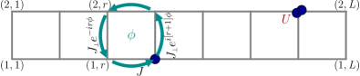
Figure 1: (Color online) Sketch of the model Eq. (1): bosons on a two-leg ladder, with $J$ and $J_{\scriptscriptstyle{\perp}}$ the hopping matrix elements along the legs and rungs, respectively, with $\phi$ the magnetic flux per plaquette, and $U$ the onsite interaction strength.

Bosons on a ladder subjected to gauge fields have been the topic of previous theoretical work Orignac and Giamarchi (2001); Cha and Shin (2011); Dhar et al. (2012, 2013); Petrescu and Le Hur (2013); Hügel and Paredes (2014); Wei and Mueller (2014); Tokuno and Georges (2014) (see also Lim et al. (2008); Möller and Cooper (2010) for 2D lattices), yet complete quantitative phase diagrams are lacking. In our work, we use DMRG to systematically explore the full dependence on $J_{\scriptscriptstyle{\perp}}$, $\phi$, and filling and, as a main result, we observe both gapped and gapless Meissner and vortex phases for strongly-interacting bosons. We focus on the gapped phases that emerge at a filling of one boson per rung, for which we present detailed results for chiral currents, the vortex density and current patterns in the vortex phase. In this Mott phase, Meissner currents are suppressed compared to superfluid phases, and can even decay to zero for an infinitely strong Hubbard interaction in the limit of large rung couplings $J_{\scriptscriptstyle{\perp}}\gg J$.

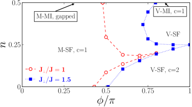
Figure 2: (Color online) Phase diagram of HCBs for $J_{\scriptscriptstyle{\perp}}/J=1$ (circles) and $J_{\scriptscriptstyle{\perp}}/J=1.5$ (squares) as a function of flux $\phi$ and density $n$ (DMRG data, $L=101$). The region $0.5<n\leq 1$ is related to the low-density regime by particle-hole symmetry.

Hamiltonian and observables. The Hamiltonian is given by (see Fig. 1):

$$H = \sum_{\ell=1,2;r=1}^{L}\left[-J\left(a^{\dagger}_{\ell,r+1}a_{\ell,r}+\textrm{H.c.}\right)+\frac{U}{2}n_{\ell,r}(n_{\ell,r}-1)\right]$$ (1)

$$-J_{\scriptscriptstyle{\perp}}\sum_{r=1}^{L}\left(e^{-ir\phi}a^{\dagger}_{1,r}a_{2,r}+\textrm{H.c.}\right)$$

on a ladder with $L$ rungs where $a^{\dagger}_{\ell,r}$ creates a boson on site $\ell=1,2$ of the $r$th rung. Energy is measured in units of $J$. We define the filling as $n=N/(2L)$, where $N$ is the total number of bosons.

On the one hand, the Hamiltonian (1) can be viewed as a minimal model for describing the edge states of a two-dimensional interacting Bose system pierced by a flux. On the other hand, we can interpret the system as a one-dimensional two-component gas Petrescu and Le Hur (2013); Hügel and Paredes (2014), where the two species are labeled with $\ell=1,2$. In the latter case, the term proportional to $J_{\scriptscriptstyle{\perp}}$ breaks the $U(1)$ symmetry related to the conservation of the particle numbers of the individual components.

Local currents will be a key quantity for characterizing different phases. We define the currents along the legs $j^{\scriptscriptstyle{\parallel}}_{\ell,r}$ and rungs $j^{\scriptscriptstyle{\perp}}_{r}$ as

$$j^{\scriptscriptstyle{\parallel}}_{\ell,r} =iJ\left(a^{\dagger}_{\ell,r+1}a_{\ell,r}-a^{\dagger}_{\ell,r}a_{\ell,r+1}\right)$$ (2)

$$j^{\scriptscriptstyle{\perp}}_{r} =iJ_{\scriptscriptstyle{\perp}}\left(e^{-ir\phi}a^{\dagger}_{1,r}a_{2,r}-e^{ir\phi}a^{\dagger}_{2,r}a_{1,r}\right)\,.$$ (3)

The chiral (or Meissner) current is $j_{\textrm{\scriptsize c}}=\partial{\cal E}_{0}/\partial\phi=\frac{1}{2L}\sum_{r}\langle j^{\scriptscriptstyle{\parallel}}_{1,r}-j^{\scriptscriptstyle{\parallel}}_{2,r}\rangle$, where ${\cal E}_{0}$ is the ground-state energy per site. Note that the operators given in Eqs. (2)-(3) depend on the gauge, but the associated expectation values are gauge invariant Möller and Cooper (2010), as can be explicitly seen in the definition of the Meissner current. For the data shown in the figures, $j_{\textrm{\scriptsize c}}$ is computed by restricting the sum to $r\in[-L/4,L/4]$ to suppress boundary effects, since in DMRG simulations we use open boundary conditions.

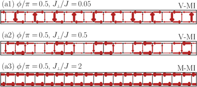
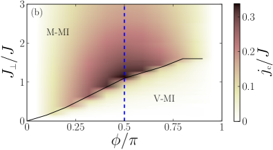
Figure 3: (Color online) (a1)-(a3) Typical current patterns for $n=0.5$, $\phi/\pi=0.5$ and $J_{\scriptscriptstyle{\perp}}/J=0.05$, 0.5 and 2 and (b) chiral current $j_{c}$ as a function of $\phi$ and $J_{\scriptscriptstyle{\perp}}$ (HCBs, $L=101$). The width of the arrows in (a1)-(a3) is proportional to the expectation values of the local currents. In (b), the solid line locates the maximum of $j_{\textrm{\scriptsize c}}=j_{\textrm{\scriptsize c}}(\phi)$ at fixed $\phi$ and the dashed line the cut considered in Fig. 4.

Phase diagram as a function of filling. Let us start by giving an account of our main results, which can be inferred from considering the limit of hard-core bosons (HCBs), i.e., $U/J=\infty$. Figure 2 shows the phase diagram for this case as a function of $n$ and $\phi$ for $J_{\scriptscriptstyle{\perp}}/J=1$ and 1.5. These results are based on a combination of a field-theory analysis and DMRG simulations for current correlation functions, the von Neumann entropy, excitation gaps, and the equation of state $n=n(\mu)$, where $\mu$ is the chemical potential.

In Fig. 2 we identify mainly four types of phases. At half-filling ($n=0.5$), there is a Mott insulator (MI) with a mass gap for any value of $\phi$ and $J_{\scriptscriptstyle{\perp}}\not=0$. At small values of $\phi$, we find a Meissner phase (M-MI) while at large $\phi$, a gapless vortex state exists (V-MI). This confirms the prediction of a Mott gap for HCBs at $n=0.5$ and $J_{\scriptscriptstyle{\perp}}\neq 0$ Vekua et al. (2003); Crépin et al. (2011) and the emergence of the Meissner currents and a vortex phase for $\phi\neq 0$ Petrescu and Le Hur (2013). At finite values of $U/J<\infty$, there will be a MI-SF transition, with critical interaction strength depending on $J_{\scriptscriptstyle{\perp}}/J$ sup . At $n<0.5$, there are superfluid phases which can again be divided into a Meissner superfluid (M-SF) and a vortex superfluid (V-SF). The terms Meissner and vortex state are justified by the existence of characteristic current patterns. Examples for $n=0.5$ are shown in Figs. 3(a1)-(a2) (V-MI) and Fig. 3(a3) (M-MI) (current patterns in the M-SF and V-SF are qualitatively similar to the ones in the M-MI and V-MI, respectively: see Figs. S4(a)-(c) sup ). The Meissner phases have vanishing rung currents $\langle j_{r}^{\scriptscriptstyle{\perp}}\rangle$ but a finite chiral current $j_{\textrm{\scriptsize c}}$, while in the vortex phase, $\langle j_{r}^{\scriptscriptstyle{\perp}}\rangle\not=0$ on finite systems, with various possible vortex patterns. The M-SF phase has one gapless mode (central charge $c=1$), while the V-SF has $c=2$. We expect M-SF and V-SF to be adiabatically connected to the corresponding phases established at weak interactions Atala et al. (2014); Tokuno and Georges (2014); Orignac and Giamarchi (2001).

The M-SF phase penetrates into the V-SF phase at intermediate values of $J_{\scriptscriptstyle{\perp}}\sim J$. The vicinity of $\phi=\pi$ is special because at $n=0.25$, a gapped charge-density-wave (CDW) phase emerges at $J_{\scriptscriptstyle{\perp}}\gtrsim 1.3J$. Once this happens, the M-SF phase touches this phase, splitting the V-SF into two lobes. Eventually, both the V-MI and the upper lobe of the V-SF phase disappear for large $J_{\scriptscriptstyle{\perp}}\gtrsim 1.7J$. For $J_{\scriptscriptstyle{\perp}}\gtrsim 1.5J$, we find a jump in density at $\phi=\pi$, from $n>0.25$ to the gapped $n=0.5$ state, which for $J_{\scriptscriptstyle{\perp}}/J\to\infty$ extends down to $n=0.25$.

Effective field theory. The nature of the phase transitions can be elucidated using bosonization. If we fix $J_{\scriptscriptstyle{\perp}}\neq 0$ and change the flux at half-filling, there is a commensurate-incommensurate (C-IC) quantum phase transition Giamarchi (2004) from a gapped ($\phi<\phi^{\textrm{\scriptsize cr}}$) to a gapless ($\phi>\phi^{\textrm{\scriptsize cr}}$) behavior of the relative phase fluctuations of the two-leg system, whereas the total density mode is always gapped for strong interactions sup . Away from $n=0.5$, the total density mode becomes immediately gapless Crépin et al. (2011) and there is a C-IC transition in the relative degrees of freedom from a gapped to a gapless behavior as a function of flux Orignac and Giamarchi (2001). This picture is confirmed by DMRG results for the von Neumann entropy (see Figs. S3 and S7 sup ) and consistent with the transitions shown in Fig. 2.

The emergence of a two-component Luttinger liquid (LL) at large values of $\phi$ becomes transparent in the low-density limit where it is connected with the development of a double-minimum structure in the single-particle dispersion $\epsilon_{k}$ for $\phi>\phi^{\textrm{\scriptsize cr}}(J_{\scriptscriptstyle{\perp}})$ Hügel and Paredes (2014); Tokuno and Georges (2014). Note that the physics at low densities is very similar to that of frustrated chains in high magnetic fields below saturation (see Arlego et al. (2011); Kolezhuk et al. (2012); Shyiko et al. (2013) and references therein). For bosons and in the limit of vanishing density, once the single-particle dispersion acquires a double-minimum, the $c=2$ LL is stabilized. To show this, we solve the low-energy scattering problem of two bosons and extract the relevant scattering lengths. There are two important scattering processes at low energy: either the two bosons belong to the same minimum of $\epsilon_{k}$ (intra-species scattering) or they belong to different minima (inter-species scattering). In 1D, the scattering length is related to the scattering phase shift via $a_{i,j}=\lim_{K\to 0}\big{[}\cot(\delta_{i,j})/K\big{]}$, where $K$ is the relative momentum of the two bosons and $i,j=1,2$ distinguish bosons belonging to the minimum in $\epsilon_{k}$ at $k<0$ or $k>0$, respectively. The scattering length is related to the amplitude of the contact potential of the two-component Bose gas $U_{i,j}(x-x^{\prime})=g_{i,j}\delta(x-x^{\prime})$ with $g_{i,j}=-2/(a_{i,j}m)$. By comparing the scattering lengths $a_{i,j}$ to each other we find that in strong coupling $a_{1,1}>a_{1,2}$, such that once the double-minimum structure appears in $\epsilon_{k}$, the $c=2$ LL is energetically preferred for $n\to 0$, consistently with the mean-field argument of Tokuno and Georges (2014) and with the DMRG results shown in Fig. 2.

Large $J_{\scriptscriptstyle{\perp}}/J$ limit. Another interesting limit amenable to an analytical treatment is the case of strong rung tunneling $J_{\scriptscriptstyle{\perp}}/J\to\infty$. In that regime we introduce a pseudo-spin-$1/2$ operator $\vec{S}_{r}$ on each rung $r$ associated to the states $(|1,0\rangle_{r}+e^{ir\phi}|0,1\rangle_{r})/\sqrt{2}\to|\downarrow\rangle_{r}$, and $|0,0\rangle_{r}\to|\uparrow\rangle_{r}$. The effective spin-$1/2$ model for the special case of $\phi=\pi$ and to first order in $J^{2}/J_{\scriptscriptstyle{\perp}}$ is sup :

$$H_{\frac{1}{2}}=\frac{J^{2}}{2|J_{\scriptscriptstyle{\perp}}|}\sum_{r}\left(2S^{z}_{r}S^{z}_{r+1}-\Big{[}S^{\scriptscriptstyle{+}}_{r}(\frac{1}{2}-S^{z}_{r+1})S^{\scriptscriptstyle{-}}_{r+2}+{\rm h.c.}\Big{]}\right)\,.$$ (4)

In this basis, $n=0.5$ corresponds to the fully polarized state $\prod_{r}|\downarrow\rangle_{r}$ and the vacuum of bosons $n=0$ corresponds to $\prod_{r}|\uparrow\rangle_{r}$, while $n=0.25$ implies a vanishing magnetization $\langle S^{z}_{r}\rangle$. The classical Néel-state $\left|...\uparrow\downarrow\uparrow\downarrow...\right\rangle$ is an eigenstate of the effective model Eq. (4) and for quarter-filling it becomes the ground state due to the dominant Ising interaction. Hence, in the vicinity of $\phi=\pi$ the ground state of bosons for $J_{\scriptscriptstyle{\perp}}/J\gg 1$ at quarter-filling ($n=0.25$) is a doubly-degenerate CDW state, which breaks translational invariance. Away from $\phi\sim\pi$, the effective model undergoes a Kosterlitz-Thouless transition at some $\phi^{\textrm{\scriptsize cr}}_{\textrm{\tiny CDW}}$ from the Néel state ($\phi^{\textrm{\scriptsize cr}}_{\textrm{\tiny CDW}}<\phi\leq\pi$) into a gapless XY phase ($\phi\leq\phi^{\textrm{\scriptsize cr}}_{\textrm{\tiny CDW}}$), the latter being characterized by $c=1$. The existence of a fully gapped CDW state at $n=0.25$ for strong $J_{\scriptscriptstyle{\perp}}/J$ in the vicinity of $\phi=\pi$ and of a direct transition from the fully gapped state to a $c=1$ phase with decreasing $\phi$ explains the tendency of the M-SF to pierce the V-SF (see Fig. 2).

The effective spin-$\frac{1}{2}$ model Eq. (4) further unveils the presence of a metamagnetic behavior just below the saturation magnetization, corresponding to a jump in the density of bosons from $n=0.25$ to $n=0.5$ at $J_{\scriptscriptstyle{\perp}}/J\to\infty$. Due to the absence of spin-inversion symmetry in Eq. (4) there is no such jump from $n=0.25$ to $n=0$. For $J_{\scriptscriptstyle{\perp}}/J<\infty$, this metamagnetic behavior survives with a jump between some $n>0.25$ to $n=0.5$, which explains the numerical data shown in Figs. S1 and S2 sup .

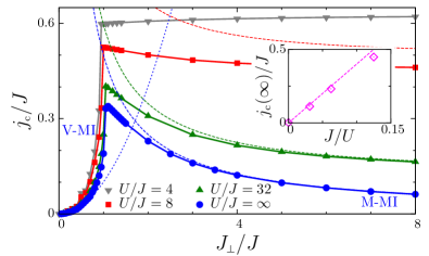
Figure 4: (Color online) Cut through the phase diagram Fig. 3(b) at $\phi/\pi=0.5$ for HCBs as well as $U/J=4$, 8 and 32. Dashed lines: Theoretical predictions for $J_{\scriptscriptstyle{\perp}}\ll J$ and $J_{\scriptscriptstyle{\perp}}\gg J$ [see Eqs. (5) and (6)]. Inset: Asymptotic value $j_{\textrm{\scriptsize c}}(J_{\scriptscriptstyle{\perp}}/J\rightarrow\infty)$ as a function of $1/U$, together with $j_{\textrm{\scriptsize c}}(\infty)=4J^{2}/U$. ($U/J<\infty$: $L=60$, $L=201$ for $U/J=\infty$).

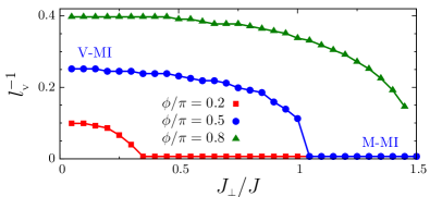
Figure 5: (Color online) Vortex density $l_{\textrm{\tiny V}}^{-1}$, i.e., inverse typical extension $l_{\textrm{\tiny V}}$ of the vortices (in lattice sites), versus $J_{\scriptscriptstyle{\perp}}$, for $\phi/\pi=0.2$, 0.5 and 0.8 ($L=101$).

Dependence of currents on $\phi$ and $J_{\scriptscriptstyle{\perp}}$. Figure 3(b) shows the chiral current as a function of $\phi$ and $J_{\scriptscriptstyle{\perp}}/J$ for HCBs at $n=0.5$. The chiral current takes a maximum at the transition from the V-MI phase to the M-MI phase. Using field theory, we derive an expression for the chiral current, in the regime $J_{\scriptscriptstyle{\perp}}\ll J$ and for small $\phi$

$$j_{\textrm{\scriptsize c}}\sim\frac{J_{\scriptscriptstyle{\perp}}^{2}}{J\phi^{3-1/K_{0}}}+O(J_{\scriptscriptstyle{\perp}}^{4})\,,$$ (5)

where $K_{0}$ is the LL parameter for the Bose-Hubbard model of decoupled chains ($J_{\scriptscriptstyle{\perp}}=0$), and ranges from $K_{0}=\infty$, for $U=0$, to $K_{0}=1$, for HCBs. The $j_{\textrm{\scriptsize c}}\propto J_{\scriptscriptstyle{\perp}}^{2}$ behavior is a generic result, valid for any repulsion $U$ and filling sup . Equation (5) implies that $j_{\textrm{\scriptsize c}}$ increases the fastest with $J_{\scriptscriptstyle{\perp}}$ at small values of $\phi$. In particular, for HCBs, we obtain $j_{\textrm{\scriptsize c}}\sim(J_{\scriptscriptstyle{\perp}}/\phi)^{2}$.

For the opposite limit of large $J_{\scriptscriptstyle{\perp}}\gg J$, we use perturbation theory at $n=0.5$ sup to derive that for $U/J\gg 1$

$$j_{\textrm{\scriptsize c}}=\frac{J^{2}(4J_{\scriptscriptstyle{\perp}}+U)^{2}}{2J_{\scriptscriptstyle{\perp}}U(2J_{\scriptscriptstyle{\perp}}+U)}\sin(\phi)\,.$$ (6)

Therefore, in the limit of infinitely strong interactions, the chiral current decays to zero in the M-MI as $j_{\textrm{\scriptsize c}}\propto 1/J_{\scriptscriptstyle{\perp}}$, contrary to the behavior at finite $U/J<\infty$ where the chiral current saturates at large $J_{\scriptscriptstyle{\perp}}\gg J$, as $j_{\textrm{\scriptsize c}}(\infty)\propto 1/U$ (see the inset in Fig. 4). This latter saturation is known from the $U=0$ limit Hügel and Paredes (2014); Atala et al. (2014) and is also observed in M-SF phases for $U\neq 0$ (results not shown).

Figure 4 presents a cut of Fig. 3 at $\phi=\pi/2$, together with finite $U/J$ data. The analytical predictions for the weak- and strong-coupling regimes from Eqs. (5) and (6) agree very well with our DMRG data for $U/J\gg 1$ [dashed lines in Fig. 4]. The essential features of the HCB case carry over to finite values of $U/J<\infty$. A finite $U$ suppresses the chiral current compared to $U=0$, which should be accessible in experiments.

The vortex phases can be further characterized by their current patterns which bear well-defined structures, with varying spatial extension and density as a function of $J_{\scriptscriptstyle{\perp}}$ and $\phi$. For the parameters of Fig. 3(a1), the sign of the current alternates along the legs, reminiscent of the chiral MI phase discussed in Dhar et al. (2012, 2013) These structures can be quantitatively studied by analyzing the rung currents $\langle j_{r}^{\scriptscriptstyle{\perp}}\rangle$. Figure 5 shows the vortex density $l_{\textrm{\tiny V}}^{-1}$ at $n=0.5$ as a function of $J_{\scriptscriptstyle{\perp}}/J$ for various values of $\phi$, where $l_{\textrm{\tiny V}}$ is the typical size of vortices extracted from the Fourier transform of the real-space patterns $\langle j_{r}^{\scriptscriptstyle{\perp}}\rangle$ over $r\in[-L/4,L/4]$. This can be interpreted as a measure of the order parameter of the transition from the Meissner into the vortex phase Orignac and Giamarchi (2001). As expected, $l_{\textrm{\tiny V}}^{-1}$ decreases to zero as the transition into the M-MI phase is approached, where only longitudinal currents survive. This is consistent with field theory predictions, which also provide that in the $J_{\scriptscriptstyle{\perp}}\ll J\phi$ limit, $l_{\textrm{\tiny V}}^{-1}\sim\phi$ sup . The rung-current correlation function $\langle j_{r}^{\scriptscriptstyle{\perp}}j_{r^{\prime}}^{\scriptscriptstyle{\perp}}\rangle$ decays algebraically in all vortex phases (see Fig. S5 sup ), unlike in the so-called chiral MI phase Dhar et al. (2012, 2013) realized for $U/J<\infty$, $\phi=\pi$, $J_{\scriptscriptstyle{\perp}}=J$, and $n=1$, which has long-range rung-current correlations.

Summary. Based on a combined DMRG and field-theoretical study, we obtained the phase diagram of strongly interacting bosons on a two-leg ladder in the presence of a homogeneous flux per plaquette. We demonstrated the existence of both gapless and gapped Meissner and vortex phases, where the gapped Meissner phase emerges in the Mott-insulating regime. The chiral current is suppressed by interactions and for HCBs it decays to zero in the M-MI, with increasing $J_{\scriptscriptstyle{\perp}}$. These results substantially extend previous studies of related models Dhar et al. (2012, 2013); Petrescu and Le Hur (2013) and confirm various predictions from field theory Orignac and Giamarchi (2001); Tokuno and Georges (2014). We provided analytical results for the weak- and strong-coupling limit, in very good agreement with numerical data. Our findings will provide guidance for future experimental studies (similar to Atala et al. (2014)) of the strongly-interacting regime. The interaction strength, density and the ratio of hopping matrix elements can routinely be tuned in optical lattice experiment Bloch et al. (2008), and so far, $\phi=\pi/2$ Aidelsburger et al. (2013); Atala et al. (2014) and $\phi=\pi$ Miyake et al. (2013) has been realized. Interesting extensions of our present study include the current patterns in harmonic traps. For this case, our results for $n=n(\mu)$ provide information about the real-space density profiles via the local density approximation. Moreover, there is the possibility to stabilize vortex solids Orignac and Giamarchi (2001), which are so far elusive in the strongly-interacting regime at incommensurate fillings. In the strong-coupling limit $U\gg J$, vortex solids are not observed in our numerical data either in the superfluid or in the $n=0.5$ Mott phase, as opposed to the $n=1$ Mott phase for moderate values of $U/J$ Dhar et al. (2012, 2013), where a vortex solid appears at $\phi=\pi$.

Note added. Very recently, two more experimental studies have investigated fermions Mancini et al. (shed) and bosons Stuhl et al. (shed) on ladders in optical lattices in the presence of artificial gauge fields.

We thank A. Paramekanti and I. Bloch for helpful discussions. The research of M.P. was supported by the European Union through the Marie-Curie grant ’ToPOL’ (No. 624033) (funded within FP7-MC-IEF). This work was also supported in part by National Science Foundation Grant No. PHYS-1066293 and the hospitality of the Aspen Center for Physics. S.G. and T.V. are supported by the QUEST (Center for Quantum Engineering and Space-Time Research) and DFG Research Training Group (Graduiertenkolleg) 1729, and I.MC. acknowledges funding from the Australian Research Council Centre of Excellence for Engineered Quantum Systems.

Supplemental Material for ’Vortex and Meissner phases of strongly-interacting bosons on a two-leg ladder’

S1 Effective Field Theory for $J_{\scriptscriptstyle{\perp}}\ll J$

For finite densities and weak rung tunneling $J_{\scriptscriptstyle{\perp}}$ we apply an effective field theory Giamarchi (2004), with the help of which we map out the ground-state phase diagram. We introduce two pairs of conjugate bosonic fields ($\theta_{\ell},\phi_{\ell}$), for $\ell=1,2$, describing, respectively, phase and density fluctuations of bosons on leg $\ell$, with commutation relations $[\theta_{\ell}(x),\partial_{y}\phi_{\ell^{\prime}}]=i\delta_{\ell,\ell^{\prime}}\delta(x-y)$. The low-energy properties of the model given in Eq. (1) of the main text are then governed by the following Hamiltonian density

$${\mathcal{H}}(x)= \frac{v_{\scriptscriptstyle{+}}}{2}\left[\frac{(\partial_{x}\phi_{\scriptscriptstyle{+}})^{2}}{K_{\scriptscriptstyle{+}}}+K_{\scriptscriptstyle{+}}(\partial_{x}\theta_{+})^{2}\right]$$ (S1)

$$+\frac{v_{\scriptscriptstyle{-}}}{2}\left[\frac{(\partial_{x}\phi_{\scriptscriptstyle{-}})^{2}}{K_{\scriptscriptstyle{-}}}+K_{\scriptscriptstyle{-}}(\partial_{x}\theta_{\scriptscriptstyle{-}}-\frac{\phi}{\sqrt{2\pi}})^{2}\right]$$

$$-\cos{\sqrt{2\pi}\theta_{\scriptscriptstyle{-}}}\sum_{m=0,1}\lambda_{m}\cos{[m\sqrt{8\pi}\phi_{\scriptscriptstyle{+}}+4m\pi nx]}$$

where $\phi_{\pm}=(\phi_{1}\pm\phi_{2})/\sqrt{2}$, $\theta_{+}=(\theta_{1}+\theta_{2})/\sqrt{2}$, $\theta_{-}=(\theta_{1}-\theta_{2}+\phi x/\sqrt{\pi})/\sqrt{2}$, and couplings constants $\lambda_{m}\sim J_{\scriptscriptstyle{\perp}}$; $K_{\pm}$ are Luttinger-liquid parameters corresponding to the total and relative fluctuations of the two-leg ladder and $v_{\pm}$ are the corresponding velocities. For $J_{\scriptscriptstyle{\perp}}\ll J$, $K_{\pm}=K_{0}(1-O(J_{\scriptscriptstyle{\perp}}^{2}))$ and $v_{\pm}=v_{0}+O(J_{\scriptscriptstyle{\perp}}^{2})$ where $K_{0}$ and $v_{0}$ are the Luttinger-liquid parameter and sound velocity for the one-dimensional Bose-Hubbard model, respectively. In particular, $K_{0}=\infty$ for $U/[Jn]\to 0$ and $K_{0}=1$ for $U/[Jn]\to\infty$. One also has $v_{0}=\alpha Ja$, where we fix the lattice constant $a=1$ in the following, where the proportionality constant $\alpha$ ranges from $\alpha\sim U/J$, for $U/[Jn]\to 0$, to $\alpha=\sin(\pi n)$ for $U/[Jn]\to\infty$.

The most important term in Eq. (S1) is the one proportional to $\lambda_{0}$, which, for small values of the flux and at any filling and interaction strength $U$, opens a gap, for arbitrarily small rung tunneling $J_{\scriptscriptstyle{\perp}}$, in the antisymmetric sector. This gap is given by $\Delta_{\scriptscriptstyle{-}}\sim J_{\scriptscriptstyle{\perp}}^{1/(2-1/(2K_{\scriptscriptstyle{-}}))}$ for $J_{\scriptscriptstyle{\perp}}\ll J$ and the interaction term pins $\langle\theta_{\scriptscriptstyle{-}}\rangle$, i.e., it locks the relative phase of bosons on the two legs as long as $\phi<\phi^{\textrm{\scriptsize cr}}$, where $\phi^{\textrm{\scriptsize cr}}$ is determined by a (soliton) gap of the antisymmetric sector. For the case of half-filling ($n=0.5$), and to unveil the role of the commensurate inter-sector interaction term $\lambda_{1}$, we apply a mean-field like decoupling that is justified due to the strongly relevant $\lambda_{0}$ coupling Vekua et al. (2004); Crépin et al. (2011). We obtain an exactly solvable effective field theory, which is a direct sum of two quantum sine-Gordon models

$${\mathcal{H}}={\mathcal{H}}^{\scriptscriptstyle{-}}_{\textrm{\tiny sG}}+{\mathcal{H}}^{\scriptscriptstyle{+}}_{\textrm{\tiny sG}},$$ (S2)

where

$${\mathcal{H}}^{\scriptscriptstyle{-}}_{\textrm{\tiny sG}}(x)= \frac{v_{\scriptscriptstyle{-}}}{2}\left[(\partial_{x}\phi_{\scriptscriptstyle{-}})^{2}+(\partial_{x}\theta_{\scriptscriptstyle{-}})^{2}\right]-2\lambda\cos{\beta\theta_{\scriptscriptstyle{-}}}$$

$$-\frac{v_{\scriptscriptstyle{-}}\beta}{2\pi}A\partial_{x}\theta_{\scriptscriptstyle{-}}+\frac{v_{\scriptscriptstyle{-}}K_{\scriptscriptstyle{-}}}{4\pi}\phi^{2},$$

with $2\lambda=\lambda_{0}+\lambda_{1}\langle\cos{\tilde{\beta}\phi_{\scriptscriptstyle{+}}}\rangle_{{\mathcal{H}}^{\scriptscriptstyle{+}}_{\textrm{\tiny sG}}}$, and

$${\mathcal{H}}^{\scriptscriptstyle{+}}_{\textrm{\tiny sG}}(x)=\frac{v_{\scriptscriptstyle{+}}}{2}\left[(\partial_{x}\phi_{\scriptscriptstyle{+}})^{2}+(\partial_{x}\theta_{\scriptscriptstyle{+}})^{2}\right]-2\tilde{\lambda}\cos{\tilde{\beta}\phi_{\scriptscriptstyle{+}}},$$

with $2\tilde{\lambda}=\lambda_{1}\langle\cos{\beta\theta_{\scriptscriptstyle{-}}}\rangle_{{\mathcal{H}}^{\scriptscriptstyle{-}}_{\textrm{\tiny sG}}}$. In the previous equation, the short-hand notations $A=\sqrt{2\pi}K_{\scriptscriptstyle{-}}\phi$, $\beta=\sqrt{2\pi/K_{\scriptscriptstyle{-}}}$ and $\tilde{\beta}=\sqrt{8\pi K_{\scriptscriptstyle{+}}}$ were introduced.

The expectation values $\langle\cos{\tilde{\beta}\phi_{\scriptscriptstyle{+}}}\rangle_{{\mathcal{H}}^{\scriptscriptstyle{+}}_{\textrm{\tiny sG}}}$ and $\langle\cos{\beta\theta_{\scriptscriptstyle{-}}}\rangle_{{\mathcal{H}}^{\scriptscriptstyle{-}}_{\textrm{\tiny sG}}}$ can be evaluated in the vacuum of the quantum sine-Gordon models in an exact way, including the phase with $\phi>\phi^{\textrm{\scriptsize cr}}$, where the antisymmetric sector contains a finite density of topological solitons (vortices) in the ground state and becomes gapless (equivalently as for the symmetric sector in the case of a finite doping away from half-filling). The vacuum energy density ${\cal E}_{0}(\lambda,\phi)$ of the quantum sine-Gordon model is known exactly Fendley et al. (1993); Zamolodchikov (1995), and the desired expectation values can be obtained from the Hellmann-Feynman theorem as $\partial_{\lambda}{\cal E}_{0}(\lambda,\phi)$. At half-filling and in the hard-core limit, $K_{\scriptscriptstyle{+}}=1-O(J_{\scriptscriptstyle{\perp}}^{2})$ and a Kosterlitz-Thouless (KT) type renormalization group analysis of the marginal perturbation (i.e., the term proportional to $\tilde{\lambda}$) shows that any rung tunneling opens a Mott gap in the symmetric sector Vekua et al. (2004); Crépin et al. (2011). The gap is exponentially small in $J_{\scriptscriptstyle{\perp}}$, for $J_{\scriptscriptstyle{\perp}}\ll J$. For finite values of $U/J<\infty$, there exists a critical value of $J_{\scriptscriptstyle{\perp}}$ and a Mott gap opens for $J_{\scriptscriptstyle{\perp}}>J_{\scriptscriptstyle{\perp}}^{\textrm{\scriptsize cr}}(U)$ via a KT phase transition at $J_{\scriptscriptstyle{\perp}}=J_{\scriptscriptstyle{\perp}}^{\textrm{\scriptsize cr}}(U)>0$ for $U/J<\infty$.

First, we consider a fixed value of the flux and discuss the limit $J_{\scriptscriptstyle{\perp}}\ll J\phi$, where the exact ground-state energy can be expanded into a perturbation series, pressumably even with a finite convergence radius Zamolodchikov (1995) as ${\cal E}_{0}=-\frac{v_{\scriptscriptstyle{-}}A^{2}}{\pi}\kappa(A,\lambda)$, where $\kappa(A,\lambda)=\kappa(\xi)=\sum_{n=1}^{\infty}\kappa_{n}\xi^{2n}$, with $\xi=\lambda/(v_{\scriptscriptstyle{-}}A^{2/(p+1)})$ and $p=\beta^{2}/(8\pi-\beta^{2})$. The expressions for the coefficients $\kappa_{n}$ are known Zamolodchikov (1995). To leading order in $J_{\scriptscriptstyle{\perp}}/J$, the vacuum energy is

$${\cal E}_{0}(A,\lambda)=-\frac{v_{\scriptscriptstyle{-}}A^{2}}{\pi}\left\{\kappa_{1}\frac{\lambda^{2}/v_{\scriptscriptstyle{-}}^{2}}{A^{(8\pi-\beta^{2})/2\pi}}+O(\xi^{4})\right\}$$ (S3)

where

$$\kappa_{1}=\pi^{2}\left(\frac{2p}{p+1}\right)^{2(p-1)/(p+1)}\frac{\Gamma\left(\frac{1-p}{1+p}\right)}{\Gamma\left(\frac{2p}{p+1}\right)}$$ (S4)

was calculated by Zamolodchikov Zamolodchikov (1995). In the hard-core limit, $\kappa_{1}=2\pi^{2}$ and it increases with decreasing $U/J$. The dependence of the chiral current on $J_{\scriptscriptstyle{\perp}}$ is given by

$$j_{\textrm{\scriptsize c}}=\frac{\partial{\cal E}_{0}(\phi,\lambda)}{\partial\phi}\simeq\frac{\kappa_{1}J_{\scriptscriptstyle{\perp}}^{2}}{J\phi^{3-1/K_{\scriptscriptstyle{-}}}}+O(J_{\scriptscriptstyle{\perp}}^{4}).$$ (S5)

Note that the proportionality to $J_{\scriptscriptstyle{\perp}}^{2}$, for $J_{\scriptscriptstyle{\perp}}\to 0$ and $\phi>0$, is completely generic, valid for any repulsion $U$ and filling. The vortex density, defined as the density of the phase slips (solitons) in the sine-Gordon model describing the relative phase fluctuations is given by $\rho_{\textrm{\tiny V}}\to\langle\partial_{x}\theta_{\scriptscriptstyle{-}}/\sqrt{\pi}\rangle_{H^{\scriptscriptstyle{-}}_{\textrm{\tiny sG}}}$ and in the limit $J_{\scriptscriptstyle{\perp}}\ll J\phi$, we have $\rho_{\textrm{\tiny V}}\sim\phi$.

Next we consider the case of a fixed rung tunneling $J_{\scriptscriptstyle{\perp}}\neq 0$ and elucidate the dependence on flux. At half filling we obtain the following picture: with increasing flux, at $\phi=\phi^{\textrm{\scriptsize cr}}$ the antisymmetric sector undergoes a commensurate-incommensurate (C-IC) quantum phase transition Giamarchi (2004) from a gapped ($\phi<\phi^{\textrm{\scriptsize cr}}$) to a gapless ($\phi>\phi^{\textrm{\scriptsize cr}}$) behavior, whereas the symmetric sector always remains gapped since $\tilde{\lambda}=\lambda_{1}\partial{\cal E}_{0}(\phi,\lambda)/\partial\lambda\neq 0$, even if $\phi\gg\phi^{\textrm{\scriptsize cr}}$, which can be seen from Eq. (S3). Therefore, at half-filling the Mott state is stable and increasing flux induces a C-IC quantum phase transition in the antisymmetric sector, from a fully gapped Meissner-Mott to a partially gapped Vortex-Mott phase. Note that $\partial{\cal E}_{0}(\phi,\lambda)/\partial\lambda=\partial{\cal E}_{0}(0,\lambda)/\partial\lambda$ is independent of $\phi$ for $\phi<\phi^{\textrm{\scriptsize cr}}$. Hence the Mott gap is independent of $\phi$ for $\phi<\phi^{\textrm{\scriptsize cr}}$. For $\phi>\phi^{\textrm{\scriptsize cr}}$, $\partial{\cal E}_{0}(\phi,\lambda)/\partial\lambda$ continuously decreases with increasing $\phi$ in the V-MI Zamolodchikov (1995), starting from its Meissner-Mott value $\partial{\cal E}_{0}(0,\lambda)/\partial\lambda$. The Mott state at $\phi<\phi^{\textrm{\scriptsize cr}}$ is similar to the rung-triplet phase Vekua et al. (2004) and can, especially for strong $J_{\scriptscriptstyle{\perp}}$, be mimicked as a direct product of $\prod_{r}(|1,0\rangle_{r}+e^{ir\phi}|0,1\rangle_{r})/\sqrt{2}$.

Away from half filling, the symmetric sector immediately becomes incommensurate and hence gapless. In addition, the value of $\phi^{\textrm{\scriptsize cr}}$ increases due to the weakened response in the coupling constant $\lambda$ from the symmetric sector. Hence, away from half filling, there is a C-IC transition in the antisymmetric sector from a gapped to a gapless behavior with increasing flux, with the symmetric sector providing an overall gapless background Orignac and Giamarchi (2001). This describes the transition from a Meissner superfluid (M-SF) to a vortex superfluid (V-SF) state at incommensurate fillings.

The vortex density is $\rho_{\textrm{\tiny V}}=0$ for $\phi<\phi^{\textrm{\scriptsize cr}}$ and beyond the C-IC phase transition at $\phi=\phi^{\textrm{\scriptsize cr}}$ upon further increasing the flux, $\rho_{\textrm{\tiny V}}$ increases with a square-root behavior which is characteristic for the C-IC transition, namely $\rho_{\textrm{\tiny V}}\sim\Theta(\phi-\phi^{\textrm{\scriptsize cr}})\sqrt{\phi-\phi^{\textrm{\scriptsize cr}}}$. The chiral current, given in Eq. (S5) behaves as described in Orignac and Giamarchi (2001), namely, it increases linearly with flux until $\phi<\phi^{\textrm{\scriptsize cr}}$ and then decreases in the vortex phase, consistent with the DMRG data shown in Fig. S8(b) for small rung tunneling. Note that $j_{\textrm{\scriptsize c}}=v_{\scriptscriptstyle{-}}K_{\scriptscriptstyle{-}}\phi/(2\pi)$ for $\phi<\phi^{\textrm{\scriptsize cr}}$ (where the vacuum of the sine-Gordon theory does not contain solitons). This is the behavior in the Meissner phases (both the M-SF and M-MI) while in the vortex phases (V-SF and V-MI) for $\phi>\phi^{\textrm{\scriptsize cr}}$, $j_{\textrm{\scriptsize c}}-v_{\scriptscriptstyle{-}}K_{\scriptscriptstyle{-}}\phi/(2\pi)\sim-\sqrt{\phi-\phi^{\textrm{\scriptsize cr}}}$.

The rung current is $\langle j^{\scriptscriptstyle{\perp}}\rangle\to\langle\sin{2\pi\theta_{\scriptscriptstyle{-}}}\rangle_{H^{\scriptscriptstyle{-}}_{\textrm{\tiny sG}}}$ and it is pinned at zero in the soliton-free vaccum of the sine-Gordon model ($\phi<\phi^{\textrm{\scriptsize cr}}$). The rung-current correlation function $\langle j^{\scriptscriptstyle{\perp}}(x)j^{\scriptscriptstyle{\perp}}(y)\rangle_{H^{\scriptscriptstyle{-}}_{\textrm{\tiny sG}}}$ decays exponentially to $0$ for $\phi<\phi^{\textrm{\scriptsize cr}}$, whereas it shows an algebraic decay in the regime $\phi>\phi^{\textrm{\scriptsize cr}}$ and incommensurate oscillations [see Fig. S5].

S2 Study of the large $J_{\scriptscriptstyle{\perp}}/J$-limit

Figure S1: (Color online) Equation of state $n=n(\mu)$ (density vs. chemical potential) of the effective spin-$\frac{1}{2}$ model Eq. (S7) for $\phi=\pi$ and $J_{\scriptscriptstyle{\perp}}/J=2$, 4, 8 and $\infty$ (curves from left to right). System size is $L=60$ with open boundary conditions. The chemical potential $\mu$ has been rescaled and shifted for clarity.

In the following we discuss the limit of strong rung tunneling $J_{\scriptscriptstyle{\perp}}/J\to\infty$ for the case of hard-core bosons.

S2.1 Effective spin Hamiltonian

In this regime and at filling $n\leq 0.5$, we may introduce a pseudo-spin-$\frac{1}{2}$ on a rung $r$ via

$$(\left|1,0\right\rangle_{r}+e^{ir\phi}\left|0,1\right\rangle_{r})/\sqrt{2}\ \to\left|\downarrow\right\rangle_{r}$$

$$\left|0,0\right\rangle_{r} \to\left|\uparrow\right\rangle_{r}.$$ (S6)

Then the effective spin-$\frac{1}{2}$ model, to second order in $J/|J_{\scriptscriptstyle{\perp}}|$, contains two terms:

$$H_{1/2}=J\,H_{1/2}^{0}+J^{2}/|J_{\scriptscriptstyle{\perp}}|\,H_{1/2}^{1}\,,$$ (S7)

which are given by

$$H_{1/2}^{0} =\cos\left(\frac{\phi}{2}\right)\,\sum_{r}\left[S^{\scriptscriptstyle{+}}_{r}S^{\scriptscriptstyle{-}}_{r+1}+{\rm h.c.}\right]$$

$$H_{1/2}^{1} =-\cos\left(\frac{\phi}{2}\right)^{2}\,\sum_{r}\left[S^{\scriptscriptstyle{+}}_{r}(1/2+S^{z}_{r+1})S^{\scriptscriptstyle{-}}_{r+2}+{\rm h.c.}\right]$$

$$\quad-\frac{1}{2}\sin\left(\frac{\phi}{2}\right)^{2}\,\sum_{r}\left[S^{\scriptscriptstyle{+}}_{r}(1/2-S^{z}_{r+1})S^{\scriptscriptstyle{-}}_{r+2}+{\rm h.c.}\right]$$

$$\quad-\frac{1+3\cos\left(\phi\right)}{2}\,\sum_{r}S^{z}_{r}S^{z}_{r+1}\,.$$

In this effective model, zero magnetization corresponds to quarter filling $n=0.25$ in the original ladder model, while the fully polarized states correspond to zero or half filling. For small fluxes the first order term $H_{1/2}^{0}$ clearly dominates and the system behaves as a one-component Luttinger-liquid, and the central charge is thus $c=1$.

S2.2 Behavior in the vicinity of $\phi=\pi$

To analyze the behavior of the system for finite fillings we use the effective model given in Eq. (S7), which simplifies at $\phi=\pi$, and includes only a correlated next-nearest neighbor hopping term and nearest-neighbor Ising-type interactions:

$$H_{1/2}=\frac{J^{2}}{2|J_{\scriptscriptstyle{\perp}}|}\sum_{r}\left(2S^{z}_{r}S^{z}_{r+1}-\Big{[}S^{\scriptscriptstyle{+}}_{r}(\frac{1}{2}-S^{z}_{r+1})S^{\scriptscriptstyle{-}}_{r+2}+{\rm h.c.}\Big{]}\right)\,.$$ (S8)

Due to the correlated hopping in effective model Eq. (S8), all tunneling processes are strongly suppressed and the Ising term proportional to $S^{z}_{r}S^{z}_{r+1}$ becomes dominant. Therefore, in the vicinity of $\phi=\pi$, the ground state at quarter filling $n=0.25$, expressed in terms of effective spin degrees of freedom, is a doubly degenerate Néel state, which in the language of bosons translates into the charge density-wave state. In the $n=n(\mu)$ curves shown in Fig. S1 this corresponds to the broad plateaux at $n=0.25$ for $\phi=\pi$ and different large values of $J_{\scriptscriptstyle{\perp}}/J$, which indicates a massive phase. When changing the flux from $\phi=\pi$, the system undergoes a transition from the Néel state ($\phi_{\textrm{\tiny CDW}}^{\textrm{\scriptsize cr}}<\phi\leq\pi$) into a gapless XY phase ($\phi\leq\phi_{\textrm{\tiny CDW}}^{\textrm{\scriptsize cr}}$) at $\phi=\phi_{\textrm{\tiny CDW}}^{\textrm{\scriptsize cr}}<\pi$. The latter phase is characterized by a central charge of $c=1$.

The effective spin-$\frac{1}{2}$ model of Eq. (S8), obtained in the $J_{\scriptscriptstyle{\perp}}/J\to\infty$ limit, reveals another interesting feature, namely metamagnetic behavior just below the saturation magnetization, which corresponds to a filling of $n=0.5$ for bosons as shown in Fig. S1. The magnetization curve exhibits a macroscopic jump to the saturation magnetization whose size increases with $J_{\scriptscriptstyle{\perp}}/J$. As one can see from Eq. (S8), for $J_{\scriptscriptstyle{\perp}}/J\to\infty$ and $n>0.25$, the ground-state energy is a linear function of $n$ and thus in the equation of state $n=n(\mu)$ (Fig. S1) the whole range of densities $0.25<n<0.5$ is unstable.

S2.3 Perturbation theory at $n=0.5$

As stated above (Sec. S1), at half filling, i.e., for one boson per rung, the Hamiltonian can easily be diagonalized in the limit $J_{\scriptscriptstyle{\perp}}/J\to\infty$ we are considering. The ground state is a product of rung triplets in this phase for any flux $\phi$ and it is non-degenerate, separated by a finite gap from excited states. In the $U/J\to\infty$ limit, there are two types of excitations. The first type involves changing the total boson number by one by putting two bosons on the same rung $\left|1,1\right\rangle_{r}$, or removing all bosons from one rung $\left|0,0\right\rangle_{r}$, both at an energy cost of $J_{\scriptscriptstyle{\perp}}$. The second type lives in the subspace of one boson per rung, and consists of exciting one rung of the ladder $r$ to a singlet $(\left|1,0\right>_{r}-e^{ir\phi}\left|0,1\right>_{r})/\sqrt{2}$, and is $2J_{\scriptscriptstyle{\perp}}$ higher in energy than the triplet. Then, in perturbation theory and to first order in $J/J_{\scriptscriptstyle{\perp}}$, restoring a weak leg tunneling allows the bosons to hop to the neighbouring site, which favors local excitations of the type $\left|1,1\right>_{r}\otimes\left|0,0\right>_{r\pm 1}$. One can then compute the expectation value of the chiral curent, which reads

$$j_{c}=\frac{J^{2}}{2J_{\scriptscriptstyle{\perp}}}\sin(\phi)\,.$$ (S9)

For finite but large $U\gg J$, besides the two types of excitations that we have discussed above for the case of $U/J\to\infty$, one has to include double occupancies with an energy $\sim U$. Retaining these three types of excited intermediate states, we calculate the ground-state energy in the lowest (i.e. second) order in the intra-leg tunneling $J$ and obtain the chiral current (as a derivative of the ground-state energy with the flux) as shown in Eq. (6) of the main text.

S3 Phase diagram

Figure S2: (Color online) Equation of state $n=n(\mu)$ of the microscopic model Eq. (1) of the main text, for $J_{\scriptscriptstyle{\perp}}/J=1.5$ and $\phi/\pi=0.4$, 0.6, 0.8 and 1 (curves from left to right). System size is $L=100$ with open boundary conditions. The chemical potential $\mu$ has been shifted for clarity.

Figure S3: (Color online) Von Neumann entropy $S_{\textrm{\tiny vN}}$ as a function of the partition size $L_{\textrm{\tiny A}}$. Example in (a) the M-SF phase ($J_{\scriptscriptstyle{\perp}}/J=1.5$, $n=0.25$ and $\phi=\pi/2$), and (b) the V-SF phase ($J_{\scriptscriptstyle{\perp}}/J=1.5$, $n=0.1$ and $\phi=0.9\pi$). The DMRG data (red dots) are obtained for $L=100$ and periodic boundary conditions on the legs. Solid black lines are fits of Eq. (S11) to the data; the fitting parameters $c$ and $g$ are given in the plots.

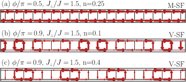
Figure S4: (Color online) Current patterns corresponding to Fig. S3 (obtained with open boundary conditions). Examples in the M-SF phase (a) for $J_{\scriptscriptstyle{\perp}}/J=1.5$, $n=0.25$ and $\phi=\pi/2$, and the V-SF phase (b) for $J_{\scriptscriptstyle{\perp}}/J=1.5$, $n=0.1$ and $\phi=0.9\pi$ and (c) for $J_{\scriptscriptstyle{\perp}}/J=1.5$, $n=0.4$ and $\phi=0.9\pi$. In (c), part of the constant leg current has been filtered out to highlight the vortex pattern.

Figure S5: (Color online) Rung-current correlation function $|\langle j^{\scriptscriptstyle{\perp}}_{r}j^{\scriptscriptstyle{\perp}}_{r^{\prime}}\rangle|$ as a function of distance $|r-r^{\prime}|$ in the V-SF phase (a) for $J_{\scriptscriptstyle{\perp}}/J=1.5$, $n=0.1$ and $\phi=0.9\pi$ and (b) for $J_{\scriptscriptstyle{\perp}}/J=1.5$, $n=0.4$ and $\phi=0.9\pi$. The solid line is a fit to the data using $|\langle j^{\scriptscriptstyle{\perp}}_{r}j^{\scriptscriptstyle{\perp}}_{r^{\prime}}\rangle|\propto 1/|r-r^{\prime}|^{\gamma}$.

In this section we present how the phase diagram, presented in Fig. 2 of the main text, has been obtained from DMRG simulations as a function of $J_{\scriptscriptstyle{\perp}}/J$ and $\phi$.

S3.1 Equation of state

Figure S2 shows typical curves of the equation of state $n=n(\mu)$, where $\mu$ is the chemical potential, for $J_{\scriptscriptstyle{\perp}}/J=1.5$ and different values of $\phi$. We see that some curves bear kinks, which are indicative of a phase transition between two gapless phases, with a change in the number of gapless excitations in Luttinger-liquid phases Okunishi and Tonegawa (2003). The curve for $\phi=0.4\pi$ has no kink, whereas the curves at $\phi=0.6$ and $0.8\pi$ have one and two kinks, respectively. The positions of those kinks are reported in Fig. 2 of the main text and yield the phase boundaries. Those curves also confirm, as stated in the main text, that the states at $n=0.5$ always have a charge gap. At $\phi=\pi$, we find that the state at $n=0.25$ is gapped, and we see the metamagnetic transition to the state at $n=0.5$. Both results are expected from the $J_{\scriptscriptstyle{\perp}}\gg J$ limit, as discussed in Sec. S2.

S3.2 Von Neumann entropy

Further insight into the phase diagram comes from a careful analysis of the von Neumann entropy

$$S_{\textrm{\tiny vN}}=-\mbox{tr}[\rho_{\textrm{\tiny A}}\mbox{ln}(\rho_{\textrm{\tiny A}})]\,$$ (S10)

where $\rho_{\textrm{\tiny A}}$ is the reduced density matrix of a subsystem of length $L_{\textrm{\tiny A}}$ in a bipartition of the full system into two parts of linear size $L_{\textrm{\tiny A}}$ and $L_{\textrm{\tiny B}}$, with $L=L_{\textrm{\tiny A}}+L_{\textrm{\tiny B}}$ (in the bipartitioning, we cut the legs at the same point). As an illustration, Fig. S3 presents $S_{\textrm{\tiny vN}}$, as a function of the partition size $L_{\textrm{\tiny A}}$ for two different points at $n\neq 0.5$. Figure S3(a) corresponds to a point in the small $\phi$ part of the phase diagram ($J_{\scriptscriptstyle{\perp}}/J=1.5$, $\phi=\pi/2$ and $n=0.25$), whereas Fig. S3(b) is located in the phase found for high-fluxes ($J_{\scriptscriptstyle{\perp}}/J=1.5$, $\phi=0.9\pi$ and $n=0.1$). In conformal field theory, the von Neumann entropy is given by Vidal et al. (2003); Calabrese and J. Cardy (2004)

$$S_{\textrm{\tiny vN}}(L_{\textrm{\tiny A}})=\frac{c}{3}\ln\left[\frac{L}{\pi}\sin\left(\pi\frac{L_{\textrm{\tiny A}}}{L}\right)\right]+g,$$ (S11)

in the case of a ladder geometry with periodic boundary conditions on the legs. The central charge $c$ determines the number of gapless excitation modes in the system, whereas $g$ is a non-universal constant. We performed fits of Eq. (S11) to the numerical data for the von Neumann entropy, which enabled us to measure $c$ and identify the different phases, thereby confirming the topology of the phase diagram. We find that the phase at low $\phi$ has $c=1$ [see, e.g., Fig. S3(a)], whereas we found $c=2$ at larger fluxes [see, e.g., Fig. S3(b)]. This is consistent with the field-theoretical analysis presented in Sec. S1 at $J_{\scriptscriptstyle{\perp}}\ll J$, from which it follows that the antisymmetric mode, which is gapped at small flux $\phi$, becomes gapless at larger fluxes, while the symmetric mode is always gapless when $n\neq 0.5$.

S3.3 Current patterns

Figures S4(a) and (b) present sketches of the current patterns corresponding to the two parameter sets analyzed in Figs. S3(a) and (b), respectively, as well as an additional one at $n=0.4$, i.e., in the upper lobe of the V-SF phase [Fig. S3(c)]. We find that the $c=1$ phase [Fig. S4(a)] has Meissner-like currents, i.e., a constant chiral current $j_{\textrm{\scriptsize c}}$ along the legs and vanishing rung currents $\langle j^{\scriptscriptstyle{\perp}}_{r}\rangle$. In the $c=2$ phase, however, we find an oscillating leg current $\langle j^{\scriptscriptstyle{\parallel}}_{\ell,r}\rangle$ and non-vanishing rung currents $\langle j^{\scriptscriptstyle{\perp}}_{r}\rangle$ [Fig. S4(b) and (c)], which corresponds to vortex patterns. This motivates us to call those phases Meissner-Superfluid (M-SF) and Vortex-Superfluid (V-SF), respectively. Figures S5(a) and (b) show the rung-current correlation function in the V-SF phase, for those two last parameter sets. We find that it indeed decreases algebraically with incommensurate oscillations, as predicted by field theory (see Sec. S1).

S4 Mott Insulating phases at $n=0.5$

Figure S6: (Color online) Gaps in the MI phases ($n=0.5$). (a1)-(b1) Mass gap $\Delta E_{\textrm{\tiny M}}$ and (a2)-(b2) excitation gap $\Delta E_{\textrm{\scriptsize ex}}$ in the subspace with constant $N$. Gaps are plotted as function of: (a1)-(a2) $J_{\scriptscriptstyle{\perp}}/J$ for $\phi/\pi=0.5$ and $\phi/\pi=0.8$, (b1)-(b2) flux $\phi$ for $J_{\scriptscriptstyle{\perp}}/J=1$. Dashed lines in (a1) and (a2) are fits of the $\phi=0.8\pi$ cuts by $\Delta E_{\textrm{\tiny M}}=J_{\scriptscriptstyle{\perp}}+A$ and $\Delta E_{\textrm{\scriptsize ex}}=2J_{\scriptscriptstyle{\perp}}+B$, respectively, with $A$ and $B$ as fitting parameters. Vertical dotted lines indicate the position of the V-MI to M-MI transition (estimated from Fig. S8). System size is $L=201$ with open boundary conditions.

Figure S7: (Color online) Von Neumann entropy $S_{\textrm{\tiny vN}}$ as a function of the partition size $L_{\textrm{\tiny A}}$. Example for (a) the M-MI phase ($J_{\scriptscriptstyle{\perp}}/J=1.5$, $n=0.5$ and $\phi=3\pi/4$), and (b) the V-MI phase ($J_{\scriptscriptstyle{\perp}}/J=1.5$, $n=0.5$ and $\phi=0.8\pi$). The DMRG data are obtained for $L=50$ and periodic boundary conditions on the legs. Solid black line on (b) is a fit of Eq. (S11) to the data; the fitting parameters $c$ and $g$ are indicated on the plots.

Figure S8: (Color online) Cuts through the phase diagram of Fig. 3(a) of the main text. (a) Cuts at $\phi/\pi=0.2$, 0.5 and 0.8, and (b) cuts at $J_{\scriptscriptstyle{\perp}}/J=1$, 2 and 3 The dashed lines are the theoretical predictions obtained for hard-core bosons when $J_{\scriptscriptstyle{\perp}}\gg J$ [see Eq. (S9)]. System size is $L=201$ with open boundary conditions.

In this section we present additional data for the Mott-insulating phases at $n=0.5$ with hard-core bosons, supporting the assertions of the main text.

S4.1 Excitation gaps

Figure S6 shows results for the mass gap

$$\Delta E_{\textrm{\tiny M}}=\frac{1}{2}\left[E_{\textrm{\scriptsize gs}}(N+1)+E_{\textrm{\scriptsize gs}}(N-1)\right]-E_{\textrm{\scriptsize gs}}(N),$$ (S12)

where $E_{\textrm{\scriptsize gs}}(N)$ is the energy of the ground state in the $N$-particles subspace, and for the excitation gap in the subspace with fixed $N$,

$$\Delta E_{\textrm{\scriptsize ex}}=E_{\textrm{\scriptsize ex}}(N)-E_{\textrm{\scriptsize gs}}(N),$$ (S13)

where $E_{\textrm{\scriptsize ex}}(N)$ is the energy of the first excited state in the $N$ particles subspace, along cuts at $\phi=0.5\pi$ and $0.8\pi$ [Figs. S6(a1) and (a2)] and along a cut at $J_{\scriptscriptstyle{\perp}}/J=1$ [Figs. S6(b1) and (b2)]. Firstly, the key result is that the mass gap is finite, which numerically we are able to resolve for $J_{\perp}\gtrsim J$. This result applies even to the V-MI phase [see, e.g., the data at $\phi=0.8\pi$ around $J_{\scriptscriptstyle{\perp}}/J\sim 1.25$ in Fig. S6(a1)], thus confirming that the system is a Mott insulator. Field theory predicts an exponentially small mass gap $\Delta E_{\textrm{\tiny M}}$ at $J_{\scriptscriptstyle{\perp}}\ll J$ (see Sec. S1 and Ref. Crépin et al. (2011)). This is hard to resolve numerically, yet the data plotted in Fig. S6(a1) indeed suggest a rapid decrease of the mass gap as $J_{\scriptscriptstyle{\perp}}$ goes to zero. In the limit of isolated rungs, $J_{\scriptscriptstyle{\perp}}\gg J$, with one boson per rung, one expects $\Delta E_{\textrm{\tiny M}}\sim J_{\scriptscriptstyle{\perp}}$ (see Sec. S2.3), which is consistent with the behaviour we find at large $J_{\scriptscriptstyle{\perp}}/J$, as highlighted by the fit of the $\phi=0.8\pi$ data by $\Delta E_{\textrm{\tiny M}}=J_{\scriptscriptstyle{\perp}}+\textrm{cst}$. Secondly, the excitation gap in the subspace with constant $N$, $\Delta E_{\textrm{\scriptsize ex}}$, vanishes whenever the system is in the V-MI phase, i.e., at small $J_{\scriptscriptstyle{\perp}}/J$ in Fig. S6(a2) and at high $\phi/\pi$ in Fig. S6(b2). In the $J_{\scriptscriptstyle{\perp}}\gg J$ limit, excitations that preserve $N$ have an energy $\Delta E_{\textrm{\scriptsize ex}}\sim 2J_{\scriptscriptstyle{\perp}}$ (see Sec. S2.3), which is consistent with the behaviour we find, as shown by the fit of $\Delta E_{\textrm{\tiny M}}=2J_{\scriptscriptstyle{\perp}}+\textrm{cst}$ to the $\phi=0.8\pi$ data in Fig. S6(a2).

S4.2 Von Neumann entropy

We now complete our investigation by analyzing the von Neumann entropy of the $n=0.5$ phases. We have carried out DMRG calculations of $S_{\textrm{\tiny vN}}$ as a function of the partition size $L_{\textrm{\tiny A}}$ (see Sec. S3.2) in the M-MI and the V-MI phases, which are presented in Figs. S7(a) and (b) respectively. In Fig. S7(a), obtained for $J_{\scriptscriptstyle{\perp}}/J=1.5$, $n=0.5$ and $\phi=3\pi/4$, the entropy saturates at a value $S_{\textrm{\tiny vN}}(L/2)$ independently of $L_{\textrm{\tiny A}}$, which is characteristic of an area law Schollwöck (2011). In Fig. S7(b), in which $J_{\scriptscriptstyle{\perp}}/J=1.5$, $n=0.5$ and $\phi=0.8\pi$, we find the typical behaviour of a gapless system with $c=1$. By fitting $S_{\textrm{\tiny vN}}(L_{\textrm{\tiny A}})$ by Eq. (S11), we obtain $c=1$. Our findings are consistent with the $J_{\scriptscriptstyle{\perp}}\ll J$ field theory of Sec. S1, which predicts that the symmetric mode is always gapped at half filling, whereas the antisymmetric mode is expected to be gapped at small flux, and can become gapless when $\phi$ increases.

S4.3 Chiral current

In Fig. S8 we provide more cuts through Fig. 3(b) of the main text, which shows the chiral current for hard-core bosons, thus complementing Fig. 4 of the main text. Figure S8(a) shows $j_{\textrm{\scriptsize c}}$ versus $J_{\scriptscriptstyle{\perp}}$ at $\phi=0.5\pi$ and $0.8\pi$. The low $J_{\scriptscriptstyle{\perp}}/J$ behaviour is quadratic $j_{\textrm{\scriptsize c}}\sim J_{\scriptscriptstyle{\perp}}^{2}$, with a prefactor that decreases with increasing flux, which is thus compatible with the prediction Eq. (S5) for small fluxes (as one has $K_{\scriptscriptstyle{-}}=1$ in the hard-core limit). The large $J_{\scriptscriptstyle{\perp}}/J$ behaviour is very well captured by standard perturbation theory [see Eq. (6) of the main text], with the asymptotic behaviour $j_{\textrm{\scriptsize c}}\sim 1/J_{\scriptscriptstyle{\perp}}$, as shown by the dashed lines. Finally, one can notice that the transition from the V-MI to the M-MI is always associated to a kink in the chiral current. Figure S8(b) shows cuts of $j_{\textrm{\scriptsize c}}$ at $J_{\scriptscriptstyle{\perp}}=J$, $2J$ and $3J$. The $j_{\textrm{\scriptsize c}}(\phi)\sim\sin(\phi)$ behaviour predicted in the $J_{\scriptscriptstyle{\perp}}\gg J$ limit [Eq. (S9)] is generic in the M-MI phase, and the transition to the V-MI phase is once again associated with a kink at $\phi^{\rm cr}$.

Figure S9: (Color online) Convergence of the von Neumann entropy for the central bipartition $S_{\textrm{\tiny vN}}(L/2)$ as a function of the dimension of the matrix product state $m$, for the parameters of Fig. S3, in the M-SF phase, where $c=1$, (squares) and in the V-SF phase, where $c=2$ (dots).

S5 Details on DMRG data

Let us finally give a few details on the numerical quality of the DMRG data that are provided in this work, where we use a finite-size DMRG algorithm Schollwöck (2005). In the calculations of currents and the equation of state $n(\mu)$ we use systems with up to $L=201$ rungs and open boundary conditions. For $U/J<\infty$, the local basis is restricted to at maximum four bosons per site, and we have checked that calculations with three bosons yield consistent results. Energies are typically converged up to the $8^{\rm th}$ digit.

Periodic boundary conditions are used for the calculation of the von Neumann entropy shown in Figs. S3 and S7. Figure S9 illustrates the convergence of $S_{\textrm{\tiny vN}}(L/2)$ as a function of the dimension of the matrix product state $m$ for the two parameter sets of Fig. S3. In general, we keep at least $m=1000$ states in the matrix product state representation, typically $m=2500$ [e.g. in Fig. S3(a)] and up to $m=4500$ where necessary [e.g. in Fig. S3(b)]. The $c=2$ states are the hardest to converge, the extraction of the central charge as $c=2$ is, however, robust, which we also verified by doing runs for open boundary conditions.

References

• Thouless et al. (1982) D. J. Thouless, M. Kohmoto, M. P. Nightingale,  and M. den Nijs, Phys. Rev. Lett. 49, 405 (1982).
• Kane and Mele (2005) C. L. Kane and E. J. Mele, Phys. Rev. Lett. 95, 146802 (2005).
• Hasan and Kane (2010) M. Z. Hasan and C. L. Kane, Rev. Mod. Phys. 82, 3045 (2010).
• Qi and Zhang (2011) X.-L. Qi and S.-C. Zhang, Rev. Mod. Phys. 83, 1057 (2011).
• Kitaev (2001) A. Kitaev, Phys.-Usp. 44, 131 (2001).
• Fu and Kane (2008) L. Fu and C. L. Kane, Phys. Rev. Lett. 100, 096407 (2008).
• Dalibard et al. (2011) J. Dalibard, F. Gerbier, G. Juzeliūnas,  and P. Öhberg, Rev. Mod. Phys. 83, 1523 (2011).
• Lin et al. (2009) Y.-J. Lin, R. L. Compton, K. Jiménez-García, J. V. Porto,  and I. B. Spielman, Nature (London) 462, 628 (2009).
• Lin et al. (2011) Y.-J. Lin, R. L. Compton, Jiménez-García, W. D. Phillips, J. V. Porto,  and I. B. Spielman, Nature Phys. 7, 531 (2011).
• Jiménez-García et al. (2012) K. Jiménez-García, L. J. LeBlanc, R. A. Williams, M. C. Beeler, A. R. Perry,  and I. B. Spielman, Phys. Rev. Lett. 108, 225303 (2012).
• Aidelsburger et al. (2011) M. Aidelsburger, M. Atala, S. Nascimbène, S. Trotzky, Y.-A. Chen,  and I. Bloch, Phys. Rev. Lett. 107, 255301 (2011).
• Struck et al. (2012) J. Struck, C. Ölschläger, M. Weinberg, P. Hauke, J. Simonet, A. Eckardt, M. Lewenstein, K. Sengstock,  and P. Windpassinger, Phys. Rev. Lett. 108, 225304 (2012).
• Aidelsburger et al. (2013) M. Aidelsburger, M. Atala, M. Lohse, J. T. Barreiro, B. Paredes,  and I. Bloch, Phys. Rev. Lett. 111, 185301 (2013).
• Miyake et al. (2013) H. Miyake, G. A. Siviloglou, C. J. Kennedy, W. C. Burton,  and W. Ketterle, Phys. Rev. Lett. 111, 185302 (2013).
• Sørensen et al. (2005) A. Sørensen, E. Demler,  and M. Lukin, Phys. Rev. Lett. 94, 086803 (2005).
• Palmer and Jaksch (2006) R. Palmer and D. Jaksch, Phys. Rev. Lett. 96, 180407 (2006).
• Hafezi et al. (2007) M. Hafezi, A. Sørensen, E. Demler,  and M. Lukin, Phys. Rev. A 76, 023613 (2007).
• Cooper (2008) N. R. Cooper, Advances in Physics 57, 539 (2008).
• Fetter (2009) A. Fetter, Rev. Mod. Phys. 81, 647 (2009).
• Möller and Cooper (2009) G. Möller and N. Cooper, Phys. Rev. Lett. 103, 105303 (2009).
• Senthil and Levin (2013) T. Senthil and M. Levin, Phys. Rev. Lett. 110, 046801 (2013).
• Regnault and Senthil (2013) N. Regnault and T. Senthil, Phys. Rev. B 88, 161106 (2013).
• Cole et al. (2012) W. S. Cole, S. Zhang, A. Paramekanti,  and N. Trivedi, Phys. Rev. Lett. 109, 085302 (2012).
• Radić et al. (2012) J. Radić, A. Di Ciolo, K. Sun,  and V. Galitski, Phys. Rev. Lett. 109, 085303 (2012).
• Cai et al. (2012) Z. Cai, X. Zhou,  and C. Wu, Phys. Rev. A 85, 061605 (2012).
• Orth et al. (2012) P. P. Orth, D. Cocks, S. Rachel, M. Buchhold, K. LeHur,  and W. Hofstetter, J. Phys. B: At. Mol. Opt. Phys. 46, 134004 (2012).
• Grusdt et al. (2013) F. Grusdt, M. Höning,  and M. Fleischhauer, Phys. Rev. Lett. 110, 260405 (2013).
• Grusdt et al. (2014) F. Grusdt, F. Letscher, M. Hafezi,  and M. Fleischhauer, Phys. Rev. Lett. 113, 155301 (2014).
• Grusdt and Höning (2014) F. Grusdt and M. Höning, Phys. Rev. A 90, 053623 (2014).
• Giamarchi (2004) T. Giamarchi, Quantum Physics in One Dimension (Clarendon Press, Oxford, 2004).
• White (1992) S. R. White, Phys. Rev. Lett. 69, 2863 (1992).
• Schollwöck (2005) U. Schollwöck, Rev. Mod. Phys. 77, 259 (2005).
• Schollwöck (2011) U. Schollwöck, Ann. Phys. (NY) 326, 96 (2011).
• Atala et al. (2014) M. Atala, M. Aidelsburger, M. Lohse, J. T. Barreiro, B. Paredes,  and I. Bloch, Nature Phys. 10, 588 (2014).
• Vekua et al. (2003) T. Vekua, G. Japaridze,  and H.-J. Mikeska, Phys. Rev. B 67, 064419 (2003).
• Crépin et al. (2011) F. Crépin, N. Laflorencie, G. Roux,  and P. Simon, Phys. Rev. B 84, 054517 (2011).
• Orignac and Giamarchi (2001) E. Orignac and T. Giamarchi, Phys. Rev. B 64, 144515 (2001).
• Cha and Shin (2011) M.-C. Cha and J.-G. Shin, Phys. Rev. A 83, 055602 (2011).
• Dhar et al. (2012) A. Dhar, M. Maji, T. Mishra, R. V. Pai, S. Mukerjee,  and A. Paramekanti, Phys. Rev. A 85, 041602 (2012).
• Dhar et al. (2013) A. Dhar, T. Mishra, M. Maji, R. V. Pai, S. Mukerjee,  and A. Paramekanti, Phys. Rev. B 87, 174501 (2013).
• Petrescu and Le Hur (2013) A. Petrescu and K. Le Hur, Phys. Rev. Lett. 111, 150601 (2013).
• Hügel and Paredes (2014) D. Hügel and B. Paredes, Phys. Rev. A 89, 023619 (2014).
• Wei and Mueller (2014) R. Wei and E. J. Mueller, Phys. Rev. A 89, 063617 (2014).
• Tokuno and Georges (2014) A. Tokuno and A. Georges, New J. Phys. 16, 073005 (2014).
• Lim et al. (2008) L.-K. Lim, C. Smith,  and A. Hemmerich, Phys. Rev. Lett. 100, 130402 (2008).
• Möller and Cooper (2010) G. Möller and N. Cooper, Phys. Rev. A 82, 063625 (2010).
• (47) See Supplemental Material.
• Arlego et al. (2011) M. Arlego, F. Heidrich-Meisner, A. Honecker, G. Rossini,  and T. Vekua, Phys. Rev. B 84, 224409 (2011).
• Kolezhuk et al. (2012) A. K. Kolezhuk, F. Heidrich-Meisner, S. Greschner,  and T. Vekua, Phys. Rev. B 85, 064420 (2012).
• Shyiko et al. (2013) I. T. Shyiko, I. P. McCulloch, J. V. Gumenjuk-Sichevska,  and A. K. Kolezhuk, Phys. Rev. B 88, 014403 (2013).
• Bloch et al. (2008) I. Bloch, J. Dalibard,  and W. Zwerger, Rev. Mod. Phys. 80, 885 (2008).
• Mancini et al. (shed) M. Mancini, G. Pagano, G. Cappellini, L. Livi, M. Rider, J. Catani, C. Sias, P. Zoller, M. Inguscio, M. Dalmonte,  and L. Fallani,  , arXiv:1502.02495 (unpublished).
• Stuhl et al. (shed) B. K. Stuhl, H.-I. Lu, L. M. Aycock, D. Genkina,  and I. B. Spielman,  , arXiv:1502.02496 (unpublished).
• Vekua et al. (2004) T. Vekua, G. I. Japaridze,  and H.-J. Mikeska, Phys. Rev. B 70, 014425 (2004).
• Fendley et al. (1993) P. Fendley, H. Saleur,  and A. B. Zamolodchikov, Int. J. Mod. Phys. A 8, 5751 (1993).
• Zamolodchikov (1995) A. B. Zamolodchikov, Int. J. Mod. Phys. A 10, 1125 (1995).
• Okunishi and Tonegawa (2003) K. Okunishi and T. Tonegawa, Phys. Rev. B 68, 224422 (2003).
• Vidal et al. (2003) G. Vidal, J. I. Latorre, E. Rico,  and A. Kitaev, Phys. Rev. Lett. 90, 227902 (2003).
• Calabrese and J. Cardy (2004) P. Calabrese and J. J. Cardy, J. Stat. Mech.: Theory Exp. , P06002 (2004).