Transverse distinguishability of entangled photons with arbitrarily shaped spatial near- and far-field distributions

Abstract

Entangled photons generated by spontaneous parametric down conversion inside a nonlinear crystal exhibit a complex spatial photon count distribution. A quantitative description of this distribution helps with the interpretation of experiments that depend on this structure. We developed a theoretical model and an accompanying numerical calculation that includes the effects of phase matching and the crystal properties to describe a wide range of spatial effects in two-photon experiments. The numerical calculation was tested against selected analytical approximations. We furthermore performed a double-slit experiment where we measured the visibility $V$ and the distinguishability $D$ and obtained $D^{2}+V^{2}=1.43$. The numerical model accurately predicts these experimental results.

I Introduction

A common source of entangled photon pairs is spontaneous parametric down conversion (SPDC)(Burnham and Weinberg, 1970), where a pump photon with frequency $\omega_{p}$, incident on a nonlinear crystal is split into two new photons. The two photons, usually referred to as signal and idler are at lower frequencies $\omega_{s},\omega_{i}<\omega_{p}$ and are entangled in multiple degrees of freedom such as energy, angular momentum and polarization. Depending on the alignment of the pump photon wave vector with respect to the optical axis of the crystal, typical cone structures of the emission directions of signal and idler photons can be observed (Fig. 1) in the Fraunhofer far-field. These are the geometric manifestation of the phase matching condition in combination with energy and momentum conservation of the signal, idler and pump photons, that maximize the efficiency of the down conversion. Due to the spatial separation of the entangled photons in the cones, SPDC is a useful tool to investigate non-classical states of light (Ou and Mandel, 1988; Fonseca et al., 1999; Friberg et al., 1985; Ghosh and Mandel, 1987; Hong and Mandel, 1986), to explore possible applications in quantum information (Neves et al., 2005) or to probe the foundations of quantum mechanics such as in the Einstein-Podolsky-Rosen paradox (Einstein et al., 1935; Howell et al., 2004).

Comprehensive theoretical descriptions of the SPDC process were developed by Mollow (Mollow, 1973) and Hong and Mandel (Hong and Mandel, 1985). An in-depth review was written by Walborn et al. (Walborn et al., 2010). These works serve as starting point for our model, that will make them applicable to describe our experiments. Our theoretical considerations allow for apertures in the near- and far-field of the nonlinear medium to manipulate the angular momentum distribution of the SPDC light. Such a framework supports the design and interpretation of experiments that study the transverse spatial structure of SPDC light in two dimensions in such detail for the first time. Related work albeit partially without considering the phase matching condition and restricted to one spatial dimension instead of two as in our case was published by Abouraddy et al. (Abouraddy et al., 2002). The far-field structure of SPDC light in two dimensions has been investigated by Bennink et al. (Bennink et al., 2006) but without our more involved inclusion of the near-field plane.

In this paper we specifically focus on spatial coincidence measurements of SPDC light. In the first section II.1 of this paper we present a theory that encompasses apertures in far and near field of the SPDC light and provides an expression for said coincidences. Their evaluation necessitates solving quite involved integral expressions. We therefore implemented a numerical simulation to obtain quantitative approximations that can be compared to experimental data. In section II.2 a set of analytical solutions that follow from various approximations are derived. These analytical solutions are used as test cases for the numerical simulation. We conclude this section with a description of a double-slit experiment with entangled photons performed by Menzel et al.(Menzel et al., 2012, 2013). We repeat this experiment which serves as a first comparison with empirical data. We finally establish in section III.2 a limit for an inequality linking the visibility $V$ of the interference fringes and the which-way distinguishability $D$ at the double slit. We observe that our experiment is closer to this limit as previously reported in (Menzel et al., 2012, 2013). This new numerical model will enable a detailed two-dimensional investigation of the fair sampling problem at a double slit (Leach et al., 2014) for both type I and type II phase matching.

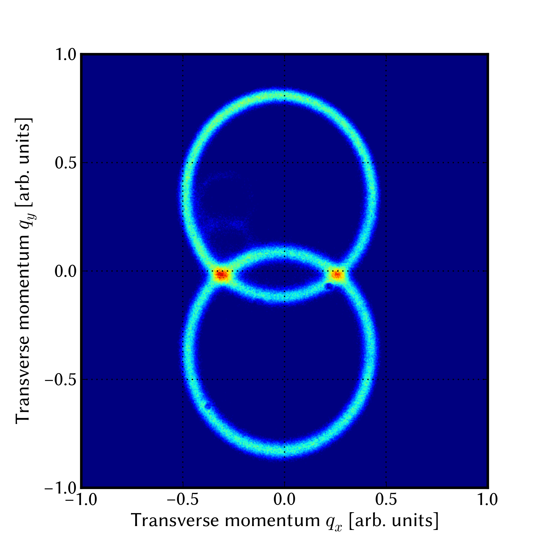
Figure 1: Typical far-field cones of the signal and idler photons generated by SPDC as measured in a plane orthogonal to the propagation direction of the pump beam.

II Materials and Methods

II.1 Theoretical Model

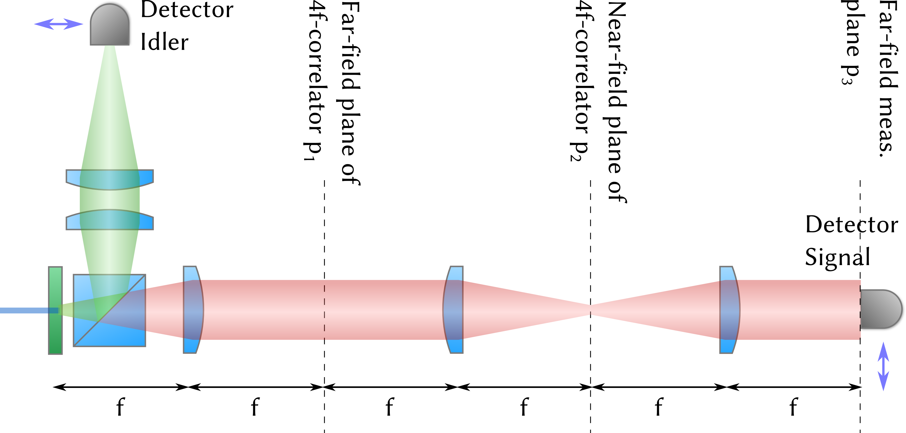
Figure 2: Schematic of a possible realization of an experiment described by our model. The entangled photons from a type II SPDC source are separated by a polarizing beam splitter (PBS) and manipulated separately by 4f-correlators. The idler path (green) is identical to the signal path (red) but is not shown to scale.

The theoretical considerations presented in this section follow the ideas outlined in (Walborn et al., 2010), which we adapted to accommodate the numerical analysis of spatial coincidence events. We start with describing the quantum state that arises from the SPDC process and we review the principal approximations. We then introduce expressions for the quantized electric field operators and the two-photon coincidence count rates which include the effects of optical elements between the crystal and the detectors. We use the terms “coincidence count rate” or “two-photon count rate” to describe the - unnormalized - probability of simultaneously detecting a signal and idler photon at given positions of the corresponding detectors.

The scope of the model is to encompass entangled two-photon experiments, where coincidence count rates are measured. We further narrow our model to a setup where two independent 4f-correlators are placed into the signal and idler beam of an SPDC source as can be seen in Fig. 2. In the respective focal planes the 4f-correlators facilitate a Fourier-transformation of the incident field (Stoler, 1982). The 4f-correlator allows us to access the near-field and the angular transverse spectrum in a single setup. The Detectors can then be positioned in the near- or far-field behind the 4f-correlators. They measure the coincidence counts in the planes $p_{1}^{(s/i)},p_{2}^{(s/i)}$ orthogonal to the propagation direction of the respective beam. The superscripts indicate if the plane is positioned in the idler or signal path. We omit the superscript in the remainder of this paper if an argument applies to both the signal and idler paths. For further reference see Fig. 2.

The signal and idler beams are separated with a polarizing beam splitter (PBS). Narrow band spectral filters are placed into both paths such that $\omega_{p}=\omega_{s}+\omega_{i}$. The angular momentum spectrum of the idler and signal beam can be manipulated independently in the far-field plane $p_{1}$ of the 4f-correlator by inserting arbitrary amplitude masks $\mathcal{T}_{s/i}(\boldsymbol{q}_{s/i}):\mathbb{R}^{2}\rightarrow\mathbb{R}$. Here $\boldsymbol{q_{s/i}}$ denotes the wavevector component of the signal/idler beam, transverse to the propagation direction. Because the first lens of the 4f-correlator establishes a simple linear mapping $\boldsymbol{q}(\boldsymbol{\rho}_{p_{1}})=\xi\boldsymbol{\rho}_{p_{1}}$ between the spatial ($\boldsymbol{\rho}_{p_{1}}$) and momentum ($\boldsymbol{q}$) coordinates in the far-field plane $p_{1}$ of the 4f-correlator, we pretend that we are manipulating the angular spectrum directly. The crystal near field is then imaged onto the near field plane $p_{2}$ of the 4f-correlator with a second amplitude mask $\mathcal{N}_{s/i}(\boldsymbol{\rho}_{s/i}):\mathbb{R}^{2}\rightarrow\mathbb{R}$. The signal and idler detectors can be placed directly behind the near-field amplitude mask at $p_{2}$ or in the far field measurement plane $p_{3}$. Arbitrary combinations of positions of the two detectors are possible. The coordinates at $p_{1}$ and $p_{3}$ are denoted by $\boldsymbol{q}_{s/i}$ and $\boldsymbol{q}_{s/i}^{\prime}$ respectively while the spatial coordinate at $p_{2}$ is $\boldsymbol{\rho}_{s/i}$. The transverse momentum coordinate of the pump beam at the plane through the center of the nonlinear crystal is $\boldsymbol{q}$ without a subscript with $\boldsymbol{\rho}$ the associated spatial coordinate.

With these conventions the quantum state of the entangled photons created by SPDC is (Walborn et al., 2010)

$$\left|\psi\right\rangle=G\iint d\boldsymbol{q}_{s}d\boldsymbol{q}_{i}\tilde{\Phi}(\boldsymbol{q}_{s},\boldsymbol{q}_{i})\left|\boldsymbol{q}_{s}\right\rangle\left|\boldsymbol{q}_{i}\right\rangle$$ (1)

The state $|\boldsymbol{q}_{s/i}\rangle$ represents a single-photon Fock state, that is characterized by its transverse momentum $\boldsymbol{q}_{s/i}$ while $k_{z}$ is fixed by the dispersion relation $k^{2}=\omega$. The constant factor G depends on the efficiency of the conversion process among other parameters which are of little interest in the context of this paper. Henceforth are going to omit these proportionality constants. The amplitude for the two photon state $\tilde{\Phi}(\boldsymbol{q}_{s},\boldsymbol{q}_{i})$ is given by

$$\tilde{\Phi}(\boldsymbol{q}_{s},\boldsymbol{q}_{i})=\tilde{u}(\boldsymbol{q}_{s}+\boldsymbol{q}_{i})\text{sinc}(\Delta k_{z}L/2)$$ (2)

where $L$ is the length of the crystal, $\Delta k_{z}=k_{zp}-k_{zs}-k_{zi}$ is the longitudinal wave vector mismatch and $\tilde{u}(\boldsymbol{q})$ is the transverse momentum spectrum of the pump beam. We define the spectrum according to

$$\tilde{u}(\boldsymbol{q})=\int d\boldsymbol{\rho}u(\boldsymbol{\rho})e^{-i\boldsymbol{\rho}\cdot\boldsymbol{q}}$$ (3)

We can interpret $u(\boldsymbol{\rho})$ as the angular electric field amplitude distribution of the pump beam. For further details on the explicit derivation of Eqs. (1)-(2) one can consult (Hong and Mandel, 1985; Walborn et al., 2010). The most important assumption that were made in (Walborn et al., 2010) are:

1. The state $\left|\psi\right\rangle$ is a first-order approximation e.g. each constituent photon state $\left|\boldsymbol{q}\right\rangle$ is a single-photon state. Effects that arise from multi-photon generation are ignored. This assumption is justified if the probability of creating more than one photon pair during a detection interval is negligible which is easily realized in SPDC experiments.

2. We assume the pump, signal and idler beams to be monochromatic which can be approximated experimentally by using narrow-band filters.

3. The quantization volume is large enough to allow the approximation of sums over $\boldsymbol{k}$ by integrals. The transverse dimensions of the crystal are larger than the transverse extent of the pump beam.

4. The beams are taken to be linearly polarized with the pump beam having extraordinary (e) polarization and the signal and idler beams having ordinary (o) polarization for type I phase matching e.g. $e\rightarrow oo$. For type II phase matching one of the down-converted fields is polarized along the e-direction e.g. $e\rightarrow oe$.

5. We ignore effects due to diffraction and refraction at the crystal’s surface and instead assume that the crystal is embedded in a medium with a matched refractive index and no birefringence. Birefringence inside the nonlinear crystal is taken into account.

The electric field operator in the paraxial approximation for a measurement directly behind the preparation stage in the plane $p_{2}$ is given by

$$\hat{\boldsymbol{E}}^{+}(\boldsymbol{\rho})=\mathcal{N}(\boldsymbol{\rho})\int d\boldsymbol{q}\mathcal{T}(\boldsymbol{q})\hat{\boldsymbol{a}}(\boldsymbol{q})\exp(i\boldsymbol{q}\cdot\boldsymbol{\rho})$$ (4)

The field operator in the far field is:

$$\hat{\boldsymbol{E}}^{+}(\boldsymbol{q}^{\prime})= \int d\boldsymbol{\rho}\exp(-i\boldsymbol{q}^{\prime}\cdot\boldsymbol{\rho})\mathcal{N}(\boldsymbol{\rho})\times$$ (5)

$$\times \int d\boldsymbol{q}\mathcal{T}(\boldsymbol{q})\hat{\boldsymbol{a}}(\boldsymbol{q})\exp(i\boldsymbol{q}\cdot\boldsymbol{\rho})$$

The coincidence detection rate or probability for simultaneously detecting an idler and a signal photon

$$C^{(2)}=\left|\hat{\boldsymbol{E}}_{s}^{(+)}\hat{\boldsymbol{E}}_{i}^{(+)}|\psi\rangle\right|^{2}$$ (6)

Thus inserting (4) and (5) into (6) yields the two-photon coincidence count rate in the near-field case

$$C^{(2)}(\boldsymbol{\rho}_{s},\boldsymbol{\rho}_{i})= \left|\mathcal{N}_{s}(\boldsymbol{\rho}_{s})\mathcal{N}_{i}(\boldsymbol{\rho}_{i})\times\right.$$ (7)

$$\times \left.\mathcal{F}^{-1}\left\{\tilde{\Phi}(\boldsymbol{q}_{s},\boldsymbol{q}_{i})\mathcal{T}_{s}(\boldsymbol{q}_{s})\mathcal{T}_{i}(\boldsymbol{q}_{i})\right\}\right|^{2}$$

In the far-field case we find the coincidence rate

$$C^{(2)}(\boldsymbol{q}_{s}^{\prime},\boldsymbol{q}_{i}^{\prime})= \mathcal{F}\left\{\mathcal{N}_{s}(\boldsymbol{\rho}_{s})\mathcal{N}_{i}(\boldsymbol{\rho}_{i})\right.\times$$ (8)

$$\times \left.\left.\mathcal{F}^{-1}\left\{\tilde{\Phi}(\boldsymbol{q}_{s},\boldsymbol{q}_{i})\mathcal{T}_{s}(\boldsymbol{q}_{s})\mathcal{T}_{i}(\boldsymbol{q}_{i})\right\}\right\}\right|^{2}$$

where $\mathcal{F}$ and $\mathcal{F}^{-1}$ denote the forward and inverse Fourier transform. These expressions are analogous to the propagation of a classical electric field in the paraxial approximation with the distinction, that the field amplitude $\tilde{\Phi}$ is a non-separable function of the transverse coordinates of the signal and the idler photons. The conditional probability of detecting a signal or idler photon is obtained by tracing out the idler or signal coordinate.

$$C^{(1)}(\boldsymbol{\rho}_{s/i})=\int d\boldsymbol{\rho}_{i/s}C^{(2)}(\boldsymbol{\rho}_{s},\boldsymbol{\rho}_{i})$$ (9)

This corresponds to the presence of a bucket detector in either the signal or idler paths. If there are no apertures $\mathcal{T}$, $\mathcal{N}$ present in the experimental setup, this quantity can be interpreted as the single-photon count rate of the signal or idler. In this particular case we call $C^{(1)}$ the “single photon count rate”. Otherwise we refer to it as the reduced coincidence count rate.

Finally, we have to account for the behavior of the longitudinal phase mismatch $\Delta k_{z}$ which is key for accurately modeling the spatial behavior of SPDC light. In a birefringent crystal the z-component of the wave vector of an extraordinary beam can be expressed (Walborn et al., 2010) in terms of its transverse components as

$$k_{z}\approx\alpha q_{x}+\eta\frac{\omega}{c_{0}}-\frac{c_{0}}{2\eta\omega}(\beta^{2}q_{x}^{2}+\gamma^{2}q_{y}^{2})$$ (10)

while for an ordinary beam

$$k_{z}\approx n_{o}\frac{\omega}{c_{0}}-\frac{c_{0}}{2n_{o}\omega}|\boldsymbol{q}|^{2}$$ (11)

Usually the quantities $\beta$ and $\gamma$ are close to unity. They cause a slight astigmatism of the down-converted fields. $\eta$ is the mean refractive index for a beam of angular frequency $\omega$. The constant $\alpha$ describes the transverse walk-off of the beam and $n_{0}=n_{o}(\omega)$ is the ordinary refractive index calculated at the angular frequency $\omega$. These expressions again are derived using the paraxial approximation.

Thus experiments that can be cast into the framework outlined above can be modeled by inserting the appropriate field operators (4),(5) into (6) with the quantum state given by (1) and the corresponding longitudinal wave vector components from Eqs. (10) and (11).

II.2 Testcase Analytic Solutions

The numerical simulation is validated against two analytical test cases. The first one is the so-called thin crystal approximation which assumes an infinitely thin crystal with $L=0$. This approximation removes the phase-matching condition $\Delta k_{z}\approx 0$ and results in an uniform transverse momentum distribution of the SPDC light. We assume that there are no apertures $\mathcal{T},\mathcal{N}$ inserted into the path of the SPDC light, the detectors are both placed in the near-field of the crystal at $p_{2}^{(s/i)}$ and the process is degenerate with $\omega_{i}=\omega_{s}$. The near-field coincidence distribution is then derived by inserting (2) into (7)

$$C^{(2)}(\boldsymbol{\rho}_{s},\boldsymbol{\rho}_{i})=\begin{cases}P|u(\boldsymbol{\rho}_{s})|^{2}&\boldsymbol{\rho}_{s}=\boldsymbol{\rho}_{i}\\ 0&\boldsymbol{\rho}_{s}\neq\boldsymbol{\rho}_{i}\end{cases}$$ (12)

$$C^{(1)}(\boldsymbol{\rho}_{s})=\int d\boldsymbol{\rho}_{i}C^{(2)}(\boldsymbol{\rho}_{s},\boldsymbol{\rho}_{i})=|u(\boldsymbol{\rho}_{s})|^{2}$$ (13)

P denotes a constant that depends on the transverse cutoff aperture. Throughout this section we use P to remind of the nonessential dependence of the absolute value of the respective expressions on the specific aperture. The signal and idler photons exhibit perfect correlations as evident from Eq. (12). The single-photon rate as seen from the signal detector reproduces the transverse intensity profile of the pump beam (13). With both detectors in the far-field plane $p_{3}$, the coincidence count and single photon rates are

$$C^{(2)}(\boldsymbol{q}_{s},\boldsymbol{q}_{i})=P\left|\tilde{u}(\boldsymbol{q}_{s}+\boldsymbol{q}_{i})\right|^{2}$$ (14)

$$C^{(1)}(\boldsymbol{q}_{s})=\int d\boldsymbol{\rho}|u(\boldsymbol{\rho})|^{2}=const$$ (15)

Thus the far-field signal coincidence rate for a fixed idler position position equals the angular spectrum of the pump beam. The resulting image is shifted by $\boldsymbol{q}_{i}$. In this case the single-photon rate of both signal and idler is constant and independent of the transverse position.

Now we consider a finite-length crystal with a plane-wave pump beam. All other parameters remain unchanged from the previous thin-crystal model. With both detectors in the far-field plane $p_{3}$, we obtain the following photon count rates.

$$C^{(2)}(\boldsymbol{q}_{s},\boldsymbol{q}_{i})=\begin{cases}P|\text{sinc}(\Delta k_{z}(\boldsymbol{q}_{s})L/2)|^{2}&\boldsymbol{q}_{s}=-\boldsymbol{q}_{i}\\ 0&\boldsymbol{q}_{s}\neq-\boldsymbol{q}_{i}\end{cases}$$ (16)

$$C^{(1)}(\boldsymbol{q}_{s})=P|\text{sinc}(\Delta k_{z}(\boldsymbol{q}_{s})L/2)|^{2}$$ (17)

Now the coincidence count rate (16) exhibits perfect anticorrelation with $\boldsymbol{q}_{s}=-\boldsymbol{q}_{i}$ as expected while displaying the typical SPDC ring structure.

Some implicit assumptions were made while deriving Eq. (12)-(17): All the formulas given here are only adequate within the limits of the paraxial approximation. The paraxial approximation is restricted to small angular frequencies $\boldsymbol{q}$. With the integrals extending from minus infinity to infinity, the paraxial approximation is insufficient on a large part of the integration domain. Some of the integrals involved are divergent. This problem has been addressed by introducing a cutoff in the integration domain. This cutoff can be justified due to the limiting apertures that are always present in an experiment. These factors account for unphysical results such as the constant single-photon count rate (15) at all angles.

II.3 Numerical Implementation

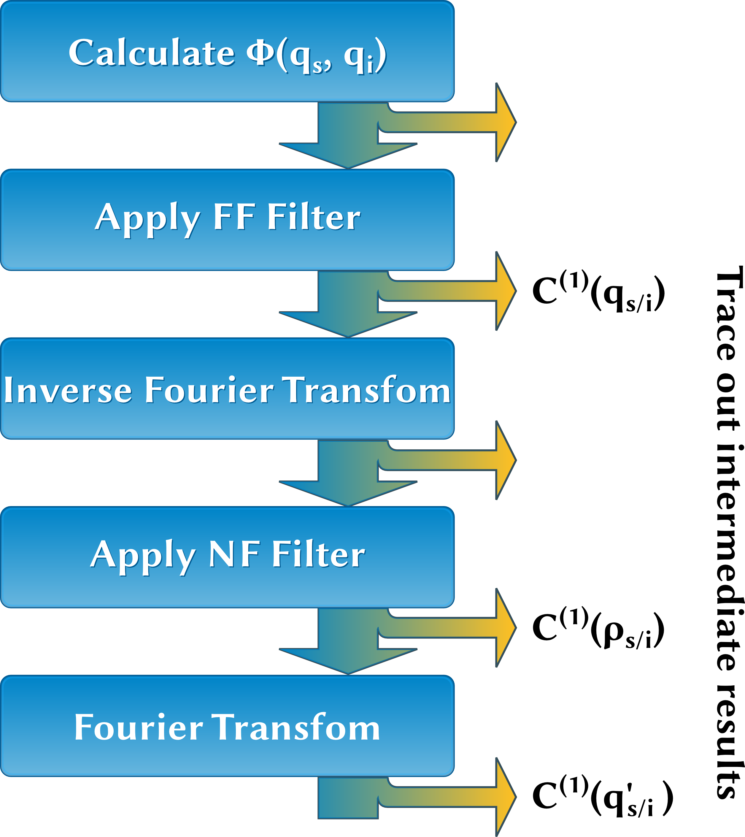
Figure 3: Flow diagram of the numerical simulation.

For reasons outlined below, we assume without loss of generality that both the signal and the idler detectors are situated in their respective far-field planes $p_{3}$ in the measurement stage. As evident from Eq. (8), the model can be thought of as a series of Fourier transforms and filtering operations on a complex four-dimensional field amplitude that propagates through the experimental setup. At each stage the intermediate two-dimensional reduced coincidence distributions $C_{s}^{(1)}$ and $C_{i}^{(1)}$ are stored. Although both detectors are assumed to be in the far-field, the numerical model yields the reduced coincidence count distributions for all planes $p_{1}$ to $p_{3}$ both before and after applying the apertures $\mathcal{T}$, $\mathcal{N}$. Using appropriate apertures, these reduced coincidence rates can be used to directly model typical two-photon experiments as outlined in section II.4.

The principal difficulty of the computation results from the $\mathcal{O}(n^{4})$ memory requirement for holding the (propagated) amplitude $\tilde{\Phi}$ in memory. With the 64 GB of RAM commonly available on today’s workstations, the simulation is thus limited to around 240 points in each of the four dimensions, assuming all calculations are made in complex double precision. All transforms are done in-place to conserve memory. Typical runtimes on a 48-core AMD Opteron System with 64 GB of RAM are around 4 minutes for a single simulation run.

Unfortunately it is impossible to directly partition the amplitude (2) into tiles and propagate those tiles independently through the experimental setup. This is due to the “each output depends on each input” property of the Fourier transform. It is possible however to split up the DFT by using a manual radix-k decimation in time or frequency. By repeatedly discarding and recalculating intermediate results, the reduced coincidence count rates can be calculated at $\mathcal{O}(k^{-4})$ the required memory at the expense of requiring $\mathcal{O}(k^{4})$ more time for a single DFT. Because the model requires two DFTs, the time tradeoff for the full propagation is $\mathcal{O}(k^{8})$ while maintaining the $\mathcal{O}(k^{-4})$ memory efficiency. An additional drawback is the complex bookkeeping required to reassemble the solution in four dimensions. Using a radix-2 decimation to perform a simulation with $N=500$ would thus take several days instead of around one hour while avoiding the need for approximately 940 GB of RAM.

A viable alternative which we applied is the use of solid state disks to cache intermediate results that do not fit into core memory. Their vastly superior access times and number of input/output operations per second enables efficient caching that is impossible to achieve with traditional rotational media. By employing two 500 GB SSDs in a RAID0 configuration, the above-mentioned simulation with $N=500$ takes approximately four days to complete and thus seems to be competitive to the manual radix-k splitting approach.

Both the Fourier transform and the filtering operation parallelize trivially and therefore benefit from using multiple threads simultaneously. The simulation was implemented in C using the FFTW library (Frigo and Johnson, 2005) for parallel in-place discrete Fourier transforms and OpenMP for concurrency. Data postprocessing and visualization was done using matplotlib, numpy and scipy (Hunter, 2007; Jones et al., 2001; Walt et al., 2011).

II.4 Double slit experiment with entangled photons

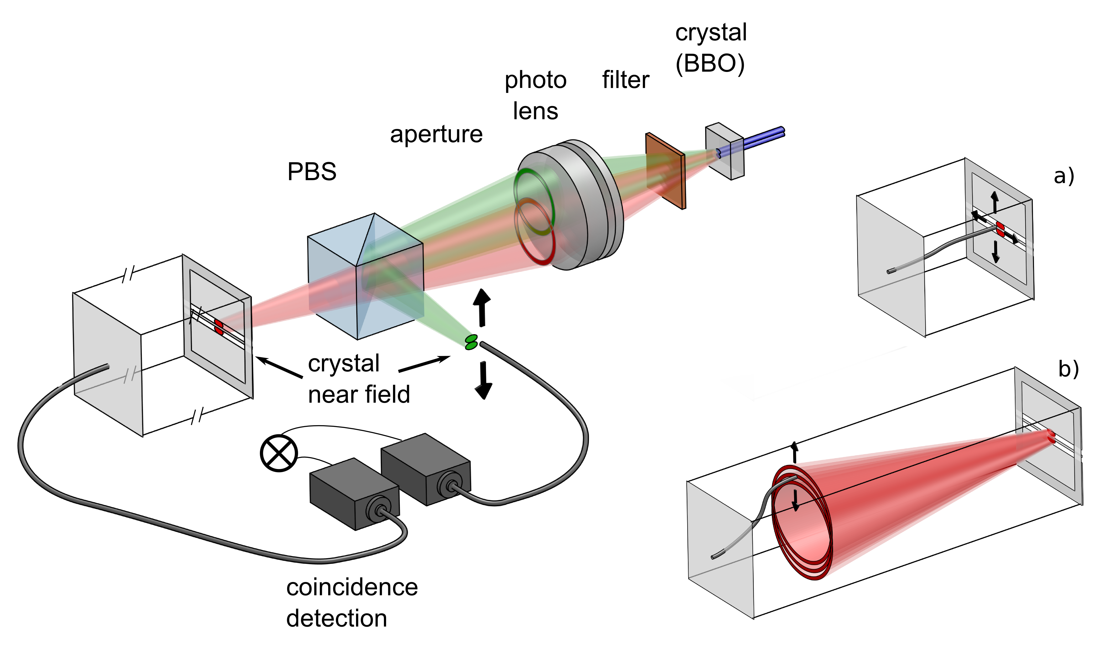
Figure 4: Schematic view of the experimental setup. The signal and idler beams are depicted in red and green respectively. Inset a) demonstrates the position of the signal detector for the near-field measurement while inset b) shows the corresponding far-field measurement.

Menzel et. al (Menzel et al., 2012) reported a double slit experiment that measured the interference fringe visibility $V$ and distinguishability $D$ for entangled photons generated by SPDC. Quantum mechanics mandates that $D^{2}+V^{2}\leq 1$, which can be interpreted as a manifestation of the duality principle (Scully et al., 1991; Englert, 1996). For brevity we will refer to it as “DV-inequality” in the remainder of the paper. The theoretical model introduced in section II.1 will be used to quantitatively analyze that experiment. We briefly review the relevant experimental facts and subsequently describe the numerical implementation.

The experimental setup is shown in Fig. 2. A 2 mm thick BBO crystal with a phase-matching angle of 42.4 degree is pumped by a TEM₀₁ beam at 404 nm. The beam is diffraction-limited while it’s width along the narrow x-axis is 140 $\mu$m. A line-pass filter at 808 nm with a full-width at half maximum filter width of 2nm is used to block all light except the degenerate signal and idler photons at 808 nm. The end facet of the crystal is then imaged onto the near-field plane of the setup using a Nikon AF 50/1.2 photographic lens. The resulting image is magnified by a factor of 2.2. A polarizing beam splitter separates the signal and idler beams. A double-slit with a center-to-center slit separation of 230 $\mu$m and a slit width of 65 $\mu$m is placed into the near-field plane of the signal path. The signal detector can be placed directly behind or in the far-field of the double slit. The idler detector can be positioned everywhere within the near-field plane. Both detectors use a gradient index multimode fiber with a core diameter of 62.5 $\mu$m. Alternatively the signal detector can be swapped out with an Andor Ixon EMCCD single-photon camera. The camera is used to record the transverse single-photon count distribution.

We perform two different experiments using the described setup. Experiment one places the Ixon camera in the far-field of the signal beam with the double slit present at the near-field plane. We then record the two-dimensional single-photon distribution $C^{(1)}(\boldsymbol{q}_{s}^{\prime})$ at $p_{3}^{(s)}$ (c.f. Fig. 2).

The second experiment is composed of two measurements which we shall denote 2a and 2b. In experiment 2a, the signal and idler detectors are both placed in the near-field plane with the double slit in the signal light path. With the idler detector fixed, the signal detector is scanned in the x-y plane behind the double slit. We calculate the which-way distinguishability

$$D=\frac{|C_{upper}^{(1)}-C_{lower}^{(1)}|}{C_{upper}^{(1)}+C_{lower}^{(1)}}$$ (18)

from the resulting 2-dimensional coincidence distribution. Here $C_{upper}^{(1)}$ is the combined coincidence rate detected at the upper slit

$$C_{upper}^{(1)}=\int\limits_{\text{upper slit}}d\boldsymbol{\rho}_{s}C^{(1)}(\boldsymbol{\rho}_{s})$$ (19)

with $C_{lower}^{(1)}$ defined analogously. We repeat this experiment for different idler positions along along the line $\rho_{ix}=0$. We thus establish a relation between the y-position of the idler detector and D. After having performed that measurement, we are in a position to make the following statement: if we detect a coincidence event with the idler detector at a given position, we can infer with a certain probability that the associated signal photon has passed through the lower (or upper) slit. Experiment 2b now places the signal detector in the far-field of the double slit. We then record a single coincidence count rate profile along the line $q_{sx}^{\prime}=0$ and calculate the visibility $V$ of the interference fringes by fitting the theoretical double slit interference function

$$C^{(1)}(\xi)=A+B\frac{\text{sinc}^{2}(\xi)}{2}\left[1+V\cos\left(\frac{2a\xi}{b}+\phi\right)\right]$$ (20)

to the profile (Menzel et al., 2012). The dimensionless variable $\xi=sq_{sx}^{\prime}$ depends linearly on the angular momentum coordinate in the far-field plane $p_{3}^{(s)}$ while the irrelevant scaling due to the particular implementation of the experiment is absorbed into the scaling factor $s$. As in 2a, we repeat the experiment for different positions of the idler detector along $\rho_{ix}=0$. We therefore obtain the relation between the visibility V of the interference fringes and the position of the idler detector. Combining the results from 2a and 2b we effectively measured the relationship between $V$ and $D$ by using the idler position as a proxy measurement of $D$. Further experimental details can be found in (Menzel et al., 2012).

These experiments can be simulated by placing a set of appropriate apertures into the numerical model. The numerical parameters for the double slit and the fiber radius differ from the experimental parameters to account for the 2.2x magnification factor of the experimental imaging system which is not present in the numerical simulation. Please refer to Fig. 2 and section II.1 for the naming conventions. The pump beam is a TEM₀₁ beam with a $4\sigma$-width of 140 $\mu$m along it’s narrow x-axis. No apertures are required in the far-field plane $p_{1}^{(s/i)}$ of our simulation e.g. $\mathcal{T}_{s/i}\equiv 1$. A double slit with a center-to-center slit separation of 105 $\mu$m and a slit width of 30 $\mu$m is placed into to signal path at $p_{2}^{(s)}$.

Experiment 1 can be simulated by omitting the idler aperture ($\mathcal{N}_{i}\equiv 1$). Then the resulting numerical $C^{(1)}(\boldsymbol{q}_{s}^{\prime})$ is equivalent to the single-photon picture recorded by the Ixon EMCCD.

Experiments 2a and 2b are emulated by placing a circular aperture with a radius of $14\mu\text{m}$ in the idler path at $p_{2}^{(i)}$. The double slit remains in the signal path. Thus the reduced coincidence count rates $C^{(1)}(\boldsymbol{\rho}_{s})$, $C^{(1)}(\boldsymbol{q}_{s}^{\prime})$ directly correspond to the respective rates introduced above. The different idler positions are simulated by displacing the center of the circular aperture.

III Results

III.1 Comparison of the numerical model against analytical solution

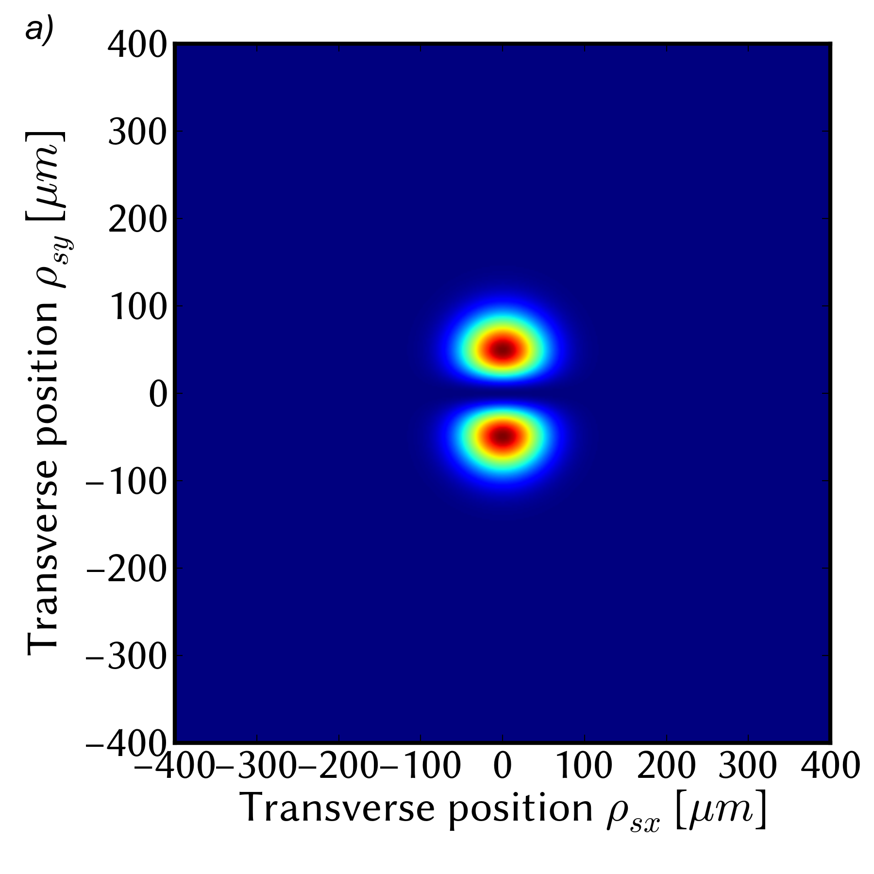
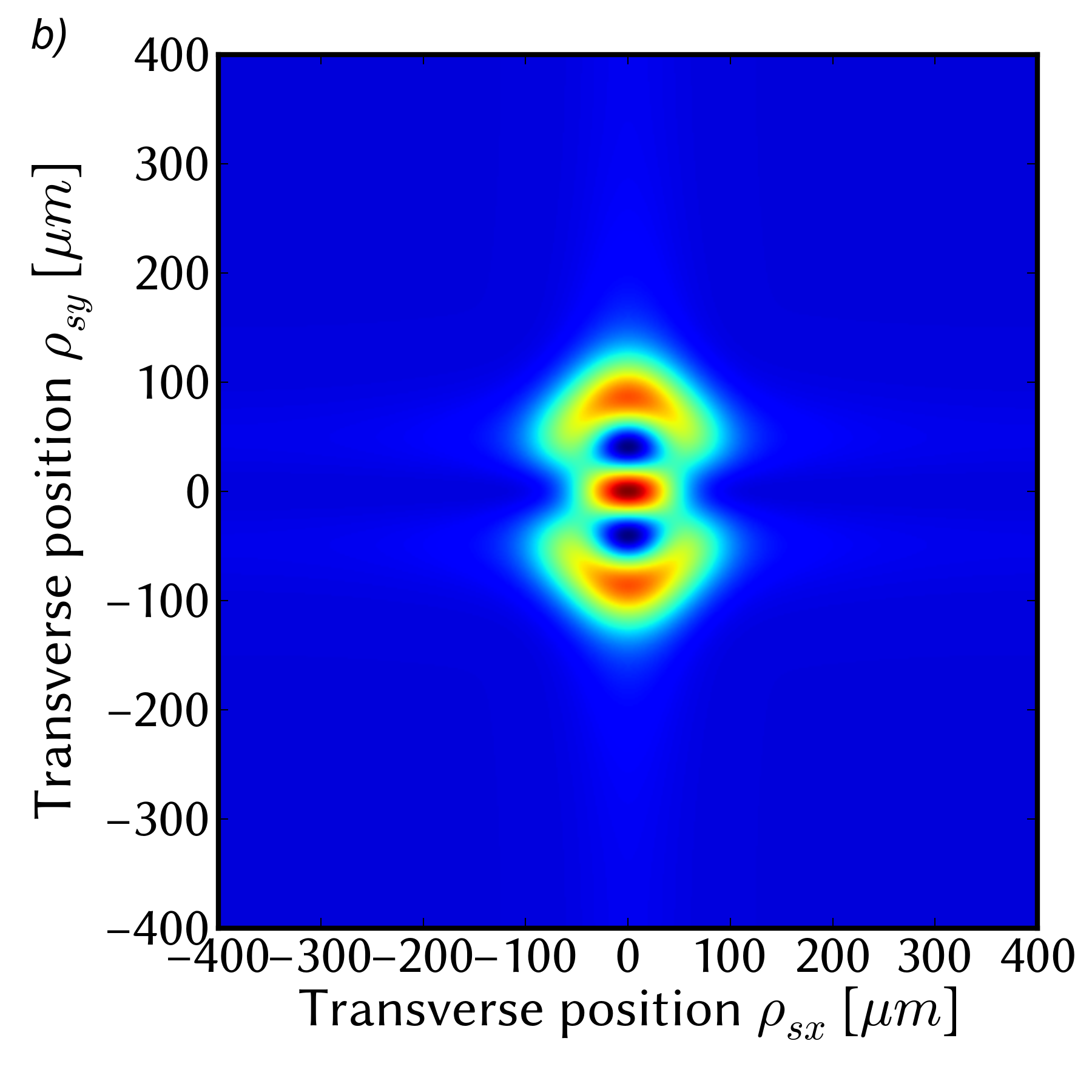
Figure 5: a) Analytically calculated signal single-photon distribution $C^{(1)}(\boldsymbol{\rho}_{s})$ in the near-field plane $p_{2}^{(s)}$. b) Deviation between numerical and analytical result with red indicating a maximum relative error of approximately $0.005$.

First we compare the numerical result to the analytical expression for the coincidence count rate in the thin-crystal approximation (12)-(15). Fig. 5 shows the analytical solution and the relative error

$$\Delta\epsilon=\frac{\left|C_{analytic}^{(1)}-C_{simulation}^{(1)}\right|}{\max\limits_{\rho}\left(C_{analytic}^{(1)}\right)}$$ (21)

of the numerical simulation in the near-field plane. The maximum relative error is smaller than $5\cdot 10^{-3}$ for $N=240$ which is the maximum resolution for 64 GB RAM. The analytical and numerical results are virtually indistinguishable. For N=500, which corresponds to approximately 937 GB of RAM, the maximum relative error decreases to $4\cdot 10^{-3}$. According to Eq. (15), the far-field count rate is expected to be constant everywhere. This behavior is reproduced by the numerical simulation.

The analytical and numerical results to the plane wave pump field approximation in the far-field are shown in Fig. 6. They exhibit a maximum relative error of the order of $3\cdot 10^{-4}$ for both N=240 and N=500.

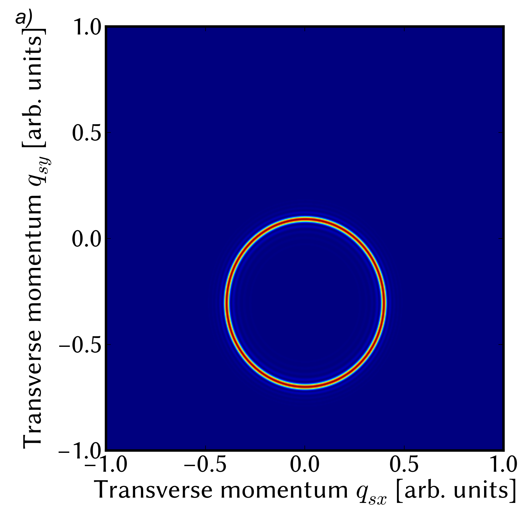
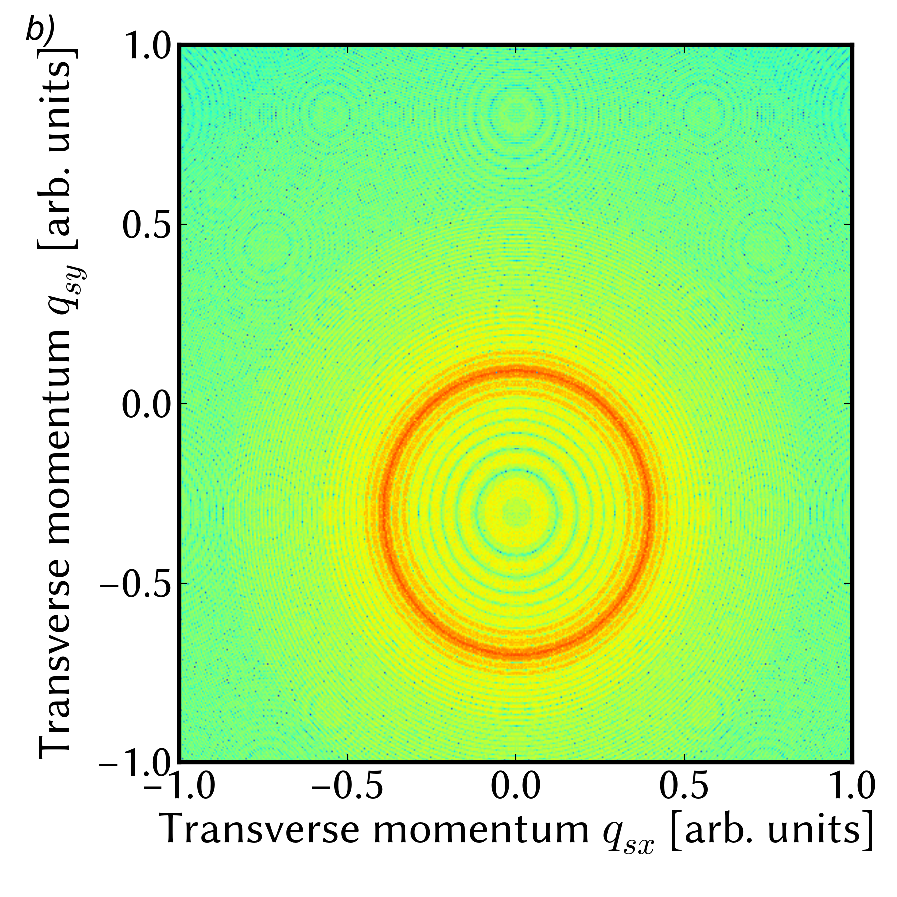
Figure 6: a) The signal single-photon distribution in the far-field as calculated from the analytic solution for N=500. b) Relative error between analytic solution and the simulation result on a logarithmic color scale [dB].

Furthermore we performed a basic consistency test (Boyd, 2001) by gradually increasing the resolution of the numerical simulation. A consistent simulation must converge towards the true solution as $N\to\infty$. Thus $\lim{}_{N\to\infty}||\tilde{\Phi}_{N}-\tilde{\Phi}_{N+1}||=0$ is a precondition for consistency. The the relative change with respect to the simulation’s resolution decreases monotonically and reaches $10^{-4}$ for $N=240$.

III.2 Experimental results and comparison to the simulation

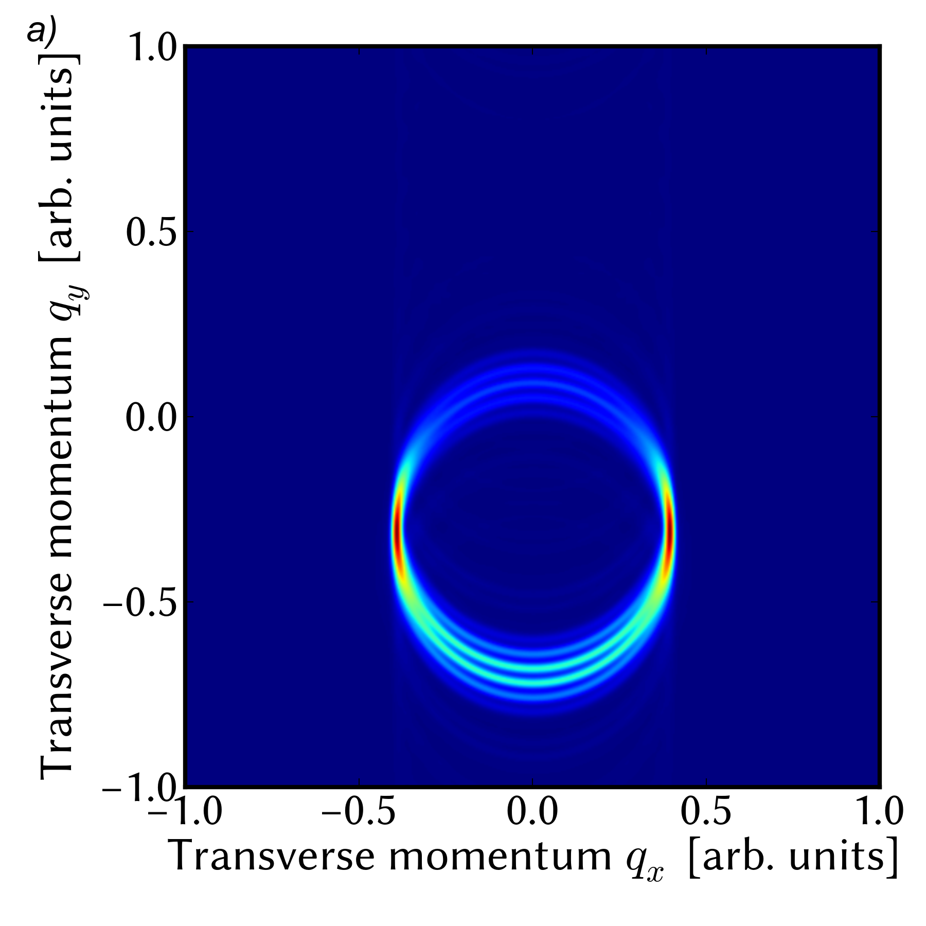
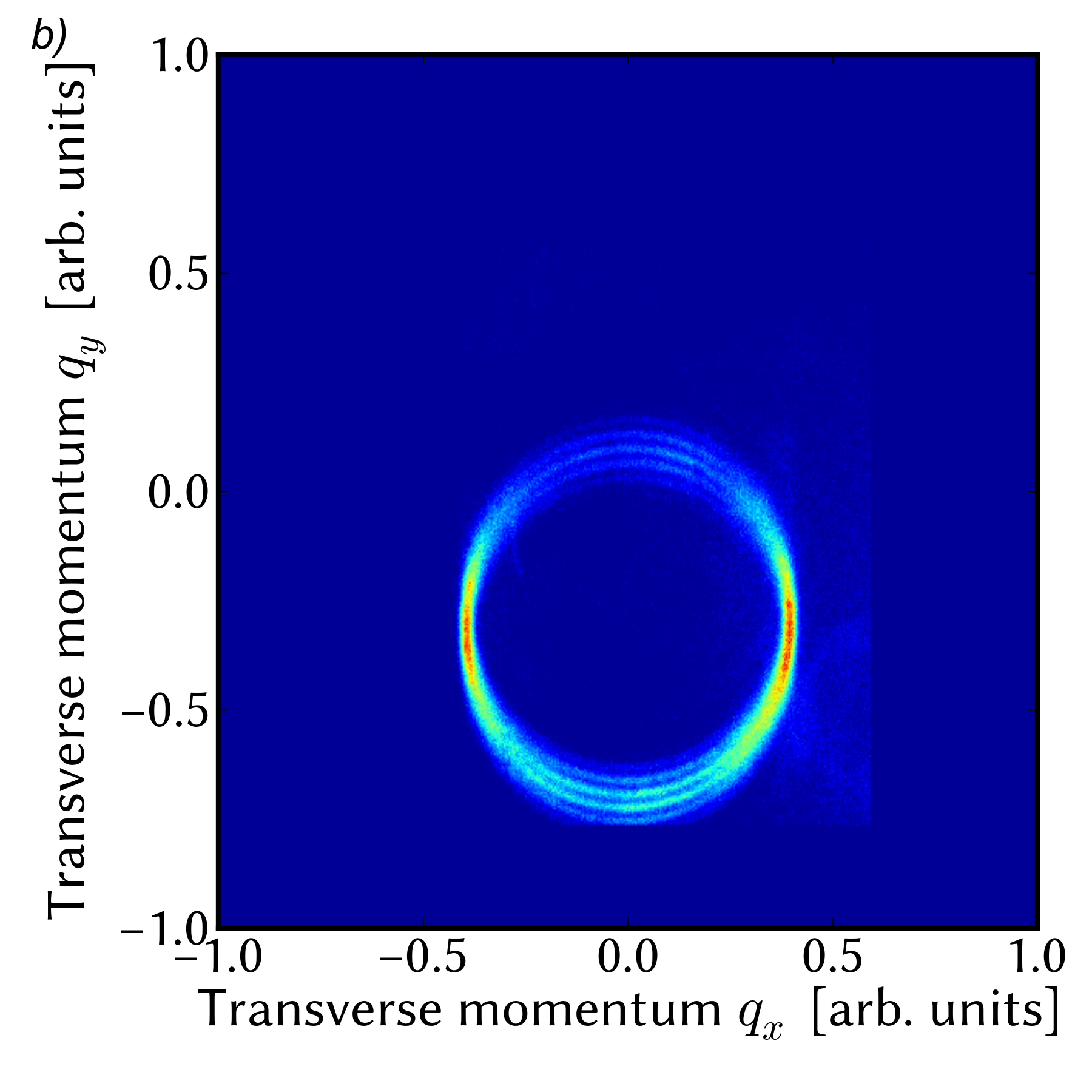
Figure 7: a) Single-photon distribution in the far-field of the double slit as calculated numerically. b) Measured single-photon distribution for the corresponding experimental setup.

The experimental single-photon rate for the first experiment outlined in section II.4 is shown in Fig. 7 on the right side. On the left side of the same figure is the result of the respective simulation. Both the simulation and the experimental photon count distribution exhibit an uneven number of interference fringes on the upper side of the ring and an even number on the lower side. Five interference fringes are clearly visible on the upper side with six on the lower side. Aside from the pronounced noise floor in the experimental data, the simulated single-photon count distributions replicate the experimental data neatly.

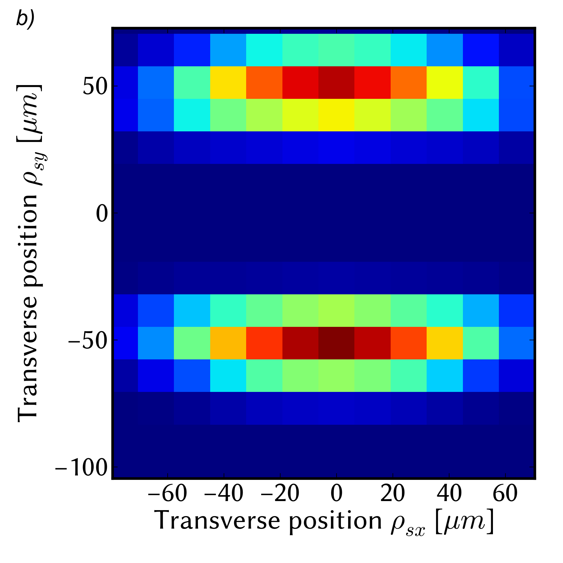
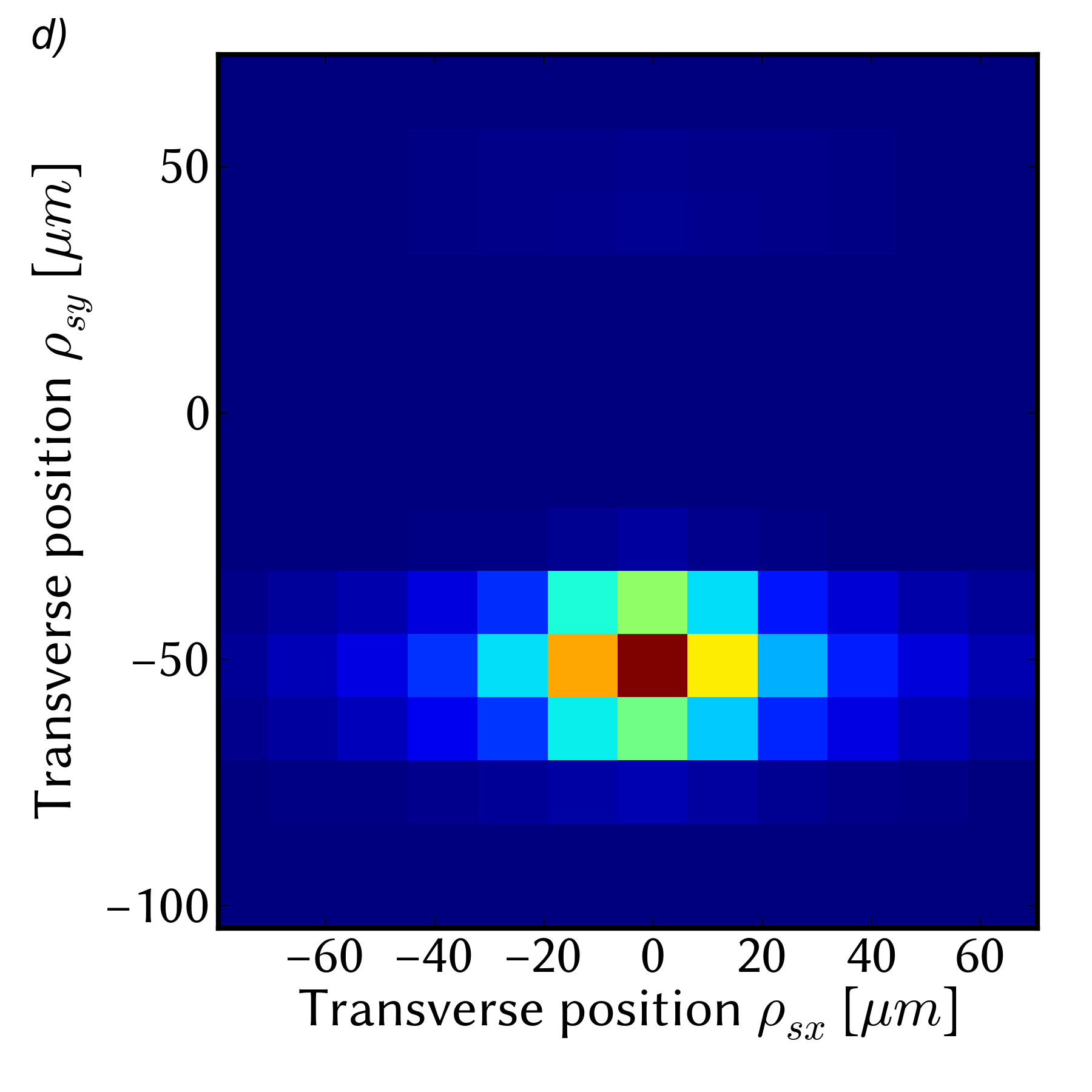
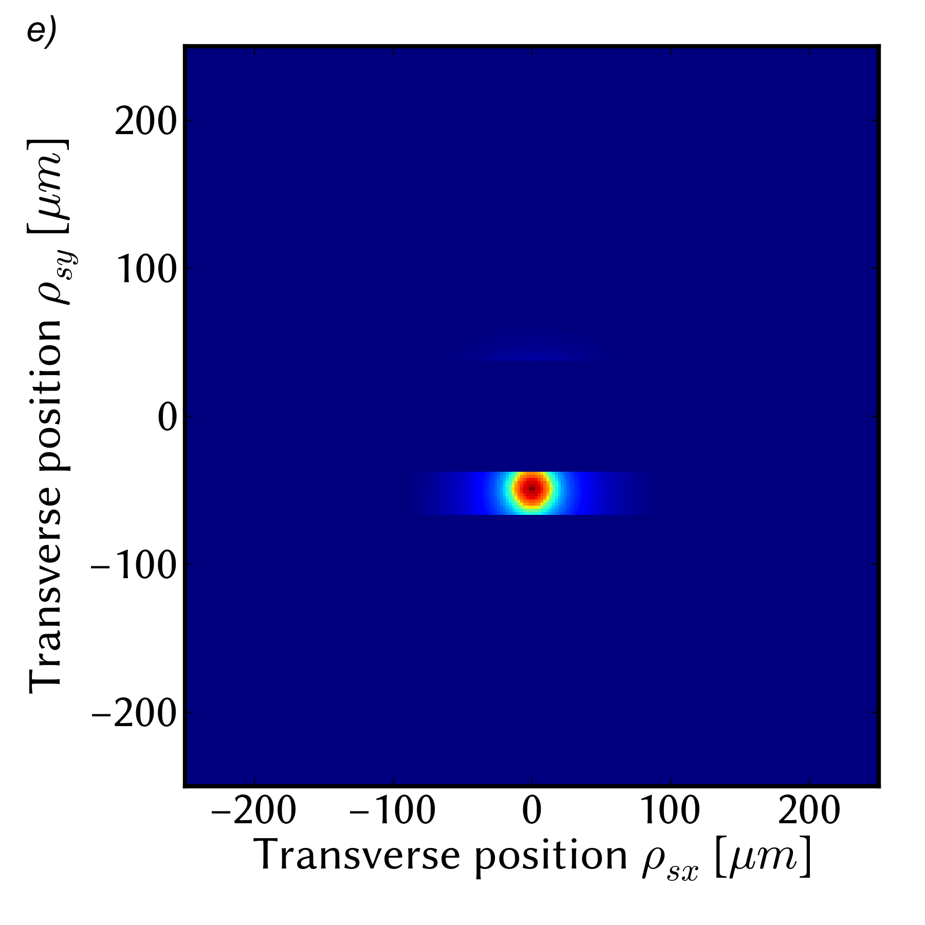
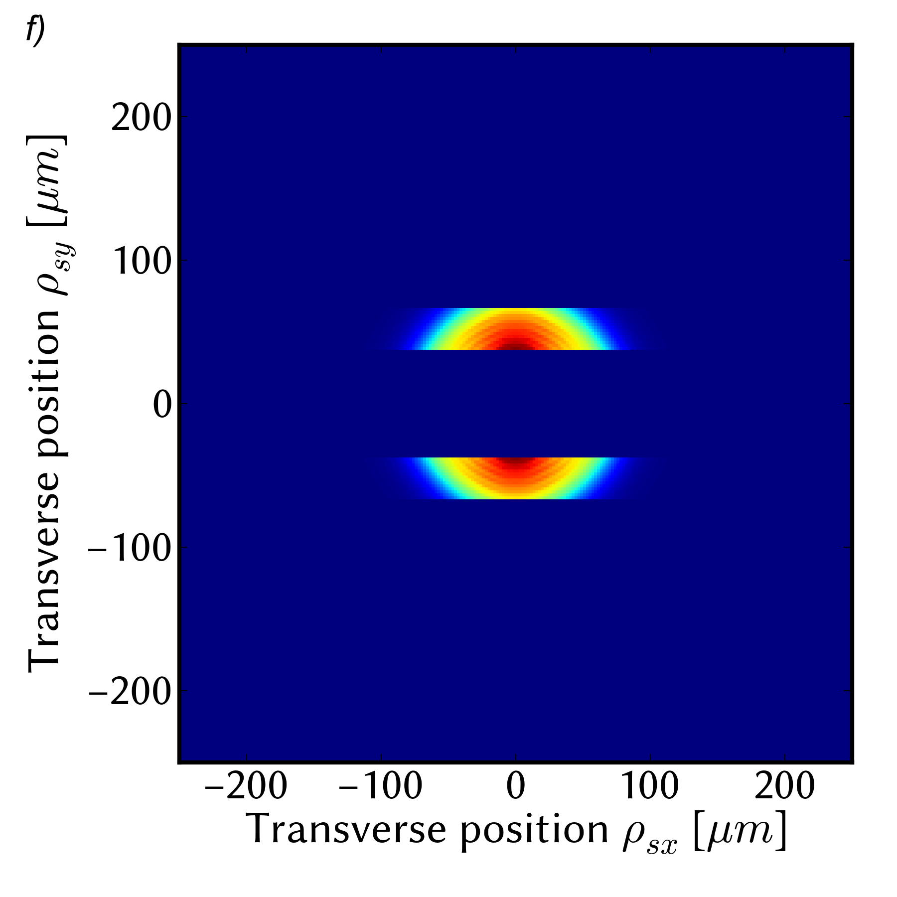
Figure 8: a) Near-field signal coincidence distribution behind the double slit with the idler detector placed in the middle between the two lobes. b) Simulated distribution with equivalent parameters to a). c) Coincidence distribution with the idler detector placed at the lower lobe of the TEM₀₁ pump beam. d) Simulated distribution with equivalent parameters to c). e) Full-resolution simulation result for d). f) Full-resolution simulation result for b). The count rates are given in arbitrary units. Each plot is normalized to unity.

We now present selected results for the experiments 2a and 2b. For the idler detector placed in between the two lobes of the TEM₀₁ mode at $(\rho_{ix},\rho_{iy})=(0,0)$, the near field coincidence distribution for the signal detector together with the numerical results can be seen in Fig 8.a and 8.b. This idler position results in a distinguishability of $D=0.0$. In addition to the coordinate transform mentioned above, the numerical result was convolved with a circular aperture kernel with a radius of 14 $\mu$m to emulate the signal fiber response. The result of the convolution was then downsampled to match the experimental sample spacing. The numerical simulation result without any transformations is shown in Fig. 8.f. Note that the finite signal fiber size must be included explicitly in a post-processing step while the idler fiber size is implicitly included in $C^{(1)}(\boldsymbol{\rho}_{s})$. Without this postprocessing, the area of the signal detector equals the intrinsic resolution limit of the simulation which in this case is $\Delta\rho_{sx}=\Delta\rho_{sy}\approx 2.1\ \mu\text{m}$.

If the idler detector is instead placed at $\rho_{iy}=-48\ \mu\text{m}$ which roughly corresponds to the middle of the lower slit, the distinguishability increases to $D\approx 0.96$ for both the simulated and experimental data. The experimental and numerical coincidence distributions are shown in Fig. 8.c and Fig. 8.d respectively with the non-transformed numerical result in Fig. 8.

Moving the signal detector into the far field and the idler detector back to $\rho_{iy}=0$ we get the simulated coincidence distribution which is displayed in Fig. 9 on the left. The simulated and measured interference fringes along the line $q_{sx}=0$ through the lower part of the ring result in visibilities of $V_{sim}=1.0$ and $V_{exp}=0.85$ respectively. This idler detector position corresponds to the figures 8 a) and b). If the idler detector is now placed again at $\rho_{iy}=-48\ \mu\text{m}$, the visibility of the interference fringes drop to $V_{exp}=0.48$ and $V_{sim}=0.58$. The simulated coincidence distribution is shown in Fig. 9 on the right. The color scales of the two plots in Fig. are individually normalized to unity. The maximum and overall coincidence count rates on the left plot are much lower when compared to the right plot. A common color scale would make the left plot indiscernible. The visibility of the interference fringes is unaffected by these absolute differences in the coincidence count rates in the absence of an additive noise floor.

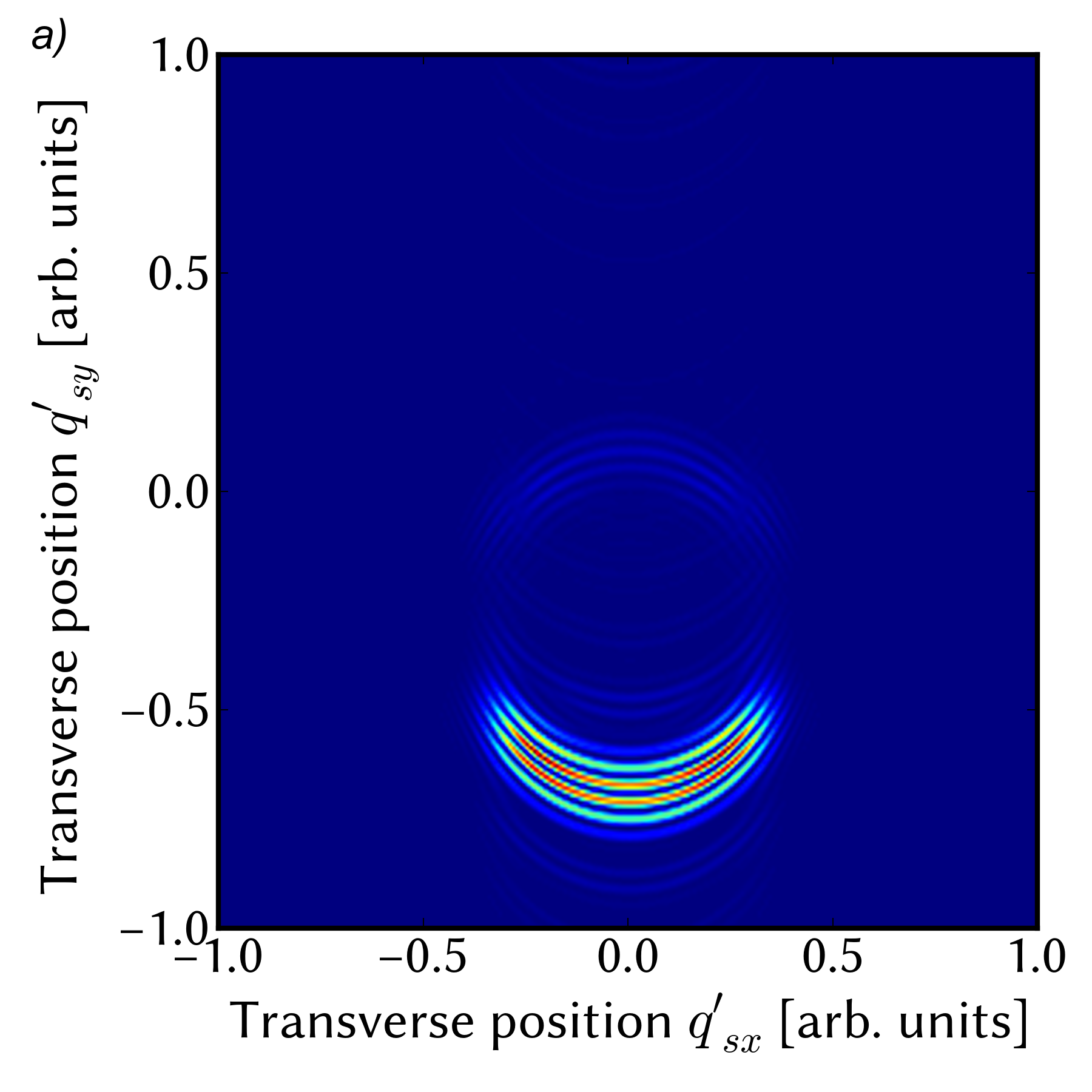
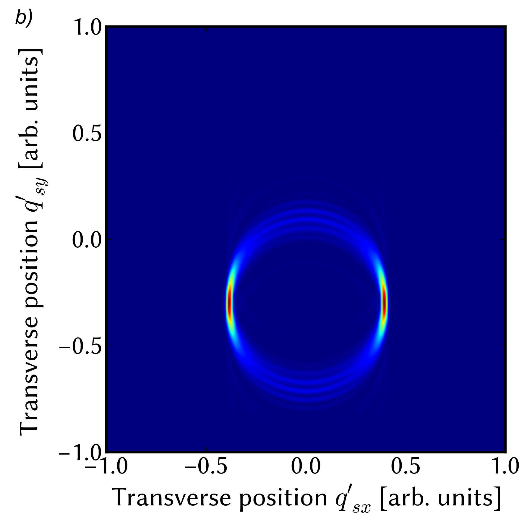
Figure 9: a) Far-field coincidence interference pattern in the signal beam with the idler detector placed between the two lobes. b) Far-field interference pattern with the idler detector placed approximately at the center of the lower lobe. Red indicates a high count rate.

The combined results from both the experiments 2a and 2b are shown in Fig. 10. The upper subfigure shows the simulated distinguishability and visibility while the measured data can be seen in the lower plot. The simulation predicts that the term $D^{2}+V^{2}$ takes on it’s maximum value of $1.47$ at $\rho_{iy}=-35\ \mu\text{m}$. Experimentally we measured $D^{2}+V^{2}=1.41$ at $\rho_{ix}=-36.5\ \mu\text{m}$.

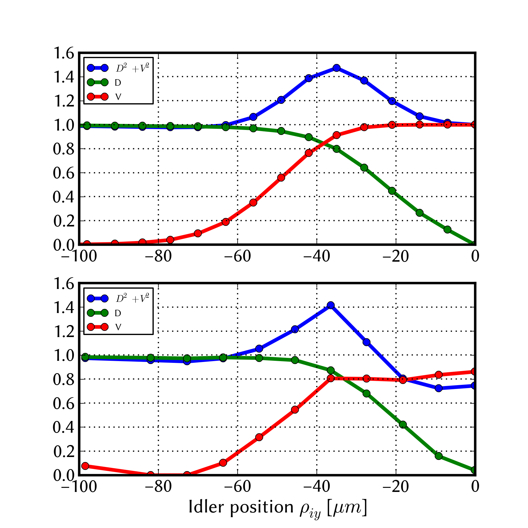
Figure 10: Distinguishability $D$, visibility $V$ and $D^{2}+V^{2}$ plotted over the position of the idler detector. Top: numerical results. Bottom: experimental data.

IV Discussion

The numerical calculations are in agreement with the analytical solutions. The analytical solutions are a test to confirm if the numerical model is able to handle simple scenarios. While the simplified analytical solutions are interesting in their own right, they have several shortcomings that make them ill-suited to predict our experimental data. The thin-crystal approximation suffers from a total absence of the phase-matching properties of the nonlinear crystal. This in turn leads to a far-field pattern that bears no resemblance to the experimentally observed count distributions, thus preventing the simulation of interference fringes that were observed in experiments one and two. The plane-wave pump field approximation suffers from a uniform near-field distribution that neglects the features of the pump beam. Our more detailed numerical model does not suffer from those limitations. Furthermore the numerical model is easily adaptable to different experimental setups by inserting the appropriate aperture functions $\mathcal{T}$ and $\mathcal{N}$ without the need to reevaluate the aperture-dependent convolutions (8). We found a resolution of $N=240$ to be sufficiently accurate to make meaningful predictions about the experimental outcome. The resolutions up to $N=500$ available with SSD caching might be required for large pump beams to retain sufficient range and resolution in both the spatial and angular momentum domains.

We simulated an optimized rerun of a recent experiment by Menzel at al. to test our numerical simulation and found the model to be in agreement with experimental data. The far-field single-photon count distribution from Fig. 7 closely matches the simulated distribution. Minor discrepancies can be attributed to the experimental noise floor. Menzel et al. (Menzel et al., 2012) previously reported a maximum value of $D^{2}+V^{2}=1.3$. Our new experiment improved on these results with $D^{2}+V^{2}=1.41$. This apparent violation of the DV-inequality was predicted by the numerical simulation which established an upper bound of $D^{2}+V^{2}=1.47$. Thus the experimental result is close to the predicted theoretical maximum for the given experimental parameters. The limiting factor hereby is the insufficient experimental resolution in the far-field measurement of the interference fringe visibility due to the signal detector fiber size.

Upon publication of (Menzel et al., 2013, 2012) it has been suggested that the experimental results were due to “leaking” photons that were not detected in the near-field measurement. In light of the experimental and theoretical results presented in this paper, we feel confident to reject the prospect of experimental errors in our experiment and (Menzel et al., 2013, 2012). While there are “leaking” photons, they alone are insufficient to explain the observed visibilities.

Note that we make no claim that the DV-inequality is invalid or that our experiment actually circumvents the duality principle. We merely demonstrated that the measurements for the given experimental setup agree excellently with theoretical predictions. A possible explanation for this mildly surprising results based on the principle of fair sampling was outlined in (Leach et al., 2014). Our numerical model provides a complete two-dimensional description of the double-slit experiment which we will use to further investigate the implications of fair sampling.

V Conclusion

We developed and implemented a quantitative model to describe the transverse spatial structure of the light fields generated by SPDC in the near and far field cases in detail. The model includes the effects of the crystal parameters such as length and phase matching angle and handles arbitrary input beams. Arbitrary amplitude manipulations of the far- and near-fields are possible in a separate preparation stage.

We repeated a double-slit experiment by Menzel et al. and improved on these results by measuring an interference fringe visibility of $V=0.8$ with a simultaneous distinguishability at the double-slit of $D=0.87$, resulting in an apparent violation of the DV-inequality with $D^{2}+V^{2}=1.41$. This is close to our predicted theoretical maximum of $D^{2}+V^{2}=1.47$. We used this experiment to test our numerical model against experimental data. We found the model to be in excellent agreement with the measured data.

Thus the numerical model can now be used to test new ideas and identify interesting parameter ranges before actually committing time to experimental work. Furthermore the numerical data can be a valuable tool to interpret the sometimes surprising results arising from experiments with entangled photons. It will provide detailed insights into the fair sampling problem at a double slit which will be discussed in a forthcoming paper.