Copyrightpage

© Copyright by Evan Alexander Johnson 2011

Abstract

The motivating question for this dissertation was to identify the minimal requirements for fluid models of plasma to allow converged simulations that agree well with converged kinetic simulations of fast magnetic reconnection. We show that truncation closure for the deviatoric pressure or for the heat flux results in singularities. Due to the strong pressure anisotropies that arise in magnetic reconnection we propose Gaussian-moment two-fluid MHD with isotropization of the pressure tensor and a Gaussian-BGK closure for the heat flux tensor as the simplest model that is likely to agree reasonably well in the diffusion region with kinetic simulations of fast magnetic reconnection.

For two-dimensional problems invariant under 180-degree rotation about the origin, we show that if the entropy production, heat flux, diffusive entropy flux, or deviatoric pressure vanishes in a neighborhood of the origin then any steady state solution with nonzero reconnection rate must be singular. In particular, models which simulate any species using a Vlasov equation or an adiabatic five-moment or ten-moment model cannot support converged steady nonsingular magnetic reconnection. Therefore, for such problems, converged simulation of steady magnetic reconnection requires that a nonzero collision operator be explicitly specified.

To study dynamic nonlinear magnetic reconnection we simulate the GEM magnetic reconnection challenge problem with an adiabatic two-fluid-Maxwell model with pressure isotropization. Our deviatoric pressure tensor agrees well with published kinetic simulations at the time of peak reconnection, but sometime thereafter the numerical solution becomes unpredictable and develops near-singularities that crash the simulation unless positivity limiters are applied. To explain these difficulties we show that steady reconnection requires heat flux and argue that sustained reconnection approximates steadily driven reconnection.

This prompts the need for a 10-moment gyrotropic heat flux closure. Using a Chapman-Enskog expansion with a Gaussian-BGK collision operator yields a heat flux closure for a magnetized 10-moment charged gas which generalizes the closure of McDonald and Groth. We argue for this closure against an entropy-respecting closure.

Chapter 1 Introduction

For convenience, most mathematical symbols are hyperlinked to the symbol glossary, which in turn references points in the text where each term is defined or discussed.

1.1 Conventions

For clarity and to avoid misunderstand we specify that

• The term “collisions” is used in the broadest possible sense to include all microscale interactions of particles with the electromagnetic field. The language of collisions is thus used in an axiomatic sense, rather than in the typically more restricted sense which refers specifically to a detailed description of particle-particle (Coulomb) interactions. In particular, it is assumed that the evolution equation of the density functions $\color[rgb]{0,0,0}f_{\mathrm{i}}(t,{\color[rgb]{0,0,0}\mathbf{x}},{\color[rgb]{0,0,0}\mathbf{v}})$ for the ions and $\color[rgb]{0,0,0}f_{\mathrm{e}}(t,{\color[rgb]{0,0,0}\mathbf{x}},{\color[rgb]{0,0,0}\mathbf{v}})$ for the electrons satisfy kinetic equations of the form

  $$\partial_{t}\color[rgb]{0,0,0}f_{\mathrm{i}} +{\color[rgb]{0,0,0}\mathbf{v}}\color[rgb]{0,0,0}{\,\bm{\cdot}\,}\color[rgb]{0,0,0}\nabla_{{\color[rgb]{0,0,0}\mathbf{x}}}\color[rgb]{0,0,0}f_{\mathrm{i}} +\color[rgb]{0,0,0}\mathbf{a}_{\mathrm{i}}\color[rgb]{0,0,0}{\,\bm{\cdot}\,}\color[rgb]{0,0,0}\nabla_{{\color[rgb]{0,0,0}\mathbf{v}}}\color[rgb]{0,0,0}f_{\mathrm{i}} =\color[rgb]{0,0,0}C^{T}_{\mathrm{i}} =\color[rgb]{0,0,0}C_{\mathrm{i}} +\color[rgb]{0,0,0}C_{\mathrm{i}\mathrm{e}},$$

  $$\partial_{t}\color[rgb]{0,0,0}f_{\mathrm{e}} +{\color[rgb]{0,0,0}\mathbf{v}}\color[rgb]{0,0,0}{\,\bm{\cdot}\,}\color[rgb]{0,0,0}\nabla_{{\color[rgb]{0,0,0}\mathbf{x}}}\color[rgb]{0,0,0}f_{\mathrm{e}} +\color[rgb]{0,0,0}\mathbf{a}_{\mathrm{e}}\color[rgb]{0,0,0}{\,\bm{\cdot}\,}\color[rgb]{0,0,0}\nabla_{{\color[rgb]{0,0,0}\mathbf{v}}}\color[rgb]{0,0,0}f_{\mathrm{e}} =\color[rgb]{0,0,0}C^{T}_{\mathrm{e}} =\color[rgb]{0,0,0}C_{\mathrm{e}} +\color[rgb]{0,0,0}C_{\mathrm{e}\mathrm{i}},$$

  where we call CTs, $\color[rgb]{0,0,0}C_{\mathrm{s}}$ and $\color[rgb]{0,0,0}C_{\mathrm{s}\mathrm{p}}$ collision operators; $\color[rgb]{0,0,0}C_{\mathrm{i}}$, $\color[rgb]{0,0,0}C_{\mathrm{e}}$, and $\color[rgb]{0,0,0}C_{\mathrm{i}\mathrm{e}}+\color[rgb]{0,0,0}C_{\mathrm{e}\mathrm{i}}$ conserve mass, momentum, and energy, and the appropriate entropy inequalities are assumed to be satisfied.

• The terms kinetic equation and Boltzmann equation are used as synonyms.

• The terms Gaussian-moment model and ten-moment model are used as synonyms.

• The terms Maxwellian-moment model and five-moment model are used as synonyms.

1.2 Plasma

A gas is a fluid composed of freely moving particles. Plasma is a gas of charged particles, which interact with the electromagnetic field. Most of the universe consists of plasma threaded by magnetic field lines. The negatively charged particles are typically electrons but may also be negatively charged dust grains. The positively charged particles are ions, typically protons or positrons. In this document we are primarily concerned with two-species plasmas, which consist of a species of positively charged particles and a species of negatively charged particles. In the case of pair plasmas, the negatively charged particles are electrons and the positively charged particles are positrons. Positrons are the antiparticles of electrons; they have the same mass but opposite charge. In the case of hydrogen plasmas, the positively charged particles are protons and the negatively charged particles are electrons. The ratio of proton mass to electron mass is large (approximately 1836).

Plasma is a type of magnetohydrodynamic fluid. A magnetohydrodynamic (MHD) fluid is a fluid that conducts electricity and has a magnetic field. In the presence of a magnetic field electrical current results in a force on the fluid perpendicular to the direction of the magnetic field and the direction of the current. An MHD description of a fluid becomes necessary when the magnetic field is strong enough to modify fluid flow (enough to affect phenomena and quantities of interest).

Each species in a plasma can be regarded as a separate fluid. One can define bulk fluid variables by appropriately summing or averaging the fluid variables of each species. Since these fluids occupy the same space, they can interact directly through frictional drag force and thermal heat exchange. The motion of a species fluid relative to the velocity of the bulk fluid is called the drift velocity of the species. A two-fluid model is used for a two-species plasma and represents each species as a distinct fluid. Two-fluid MHD regards the (bulk) MHD fluid as composed of positively and negatively charged fluids whose charge densities are assumed to cancel.

Magnetic field evolution is determined by the electric field. The electric field is given by Ohm’s law, which specifies the electric field in terms of electrical current, magnetic field, fluid velocity, and the pressures of the positive and negative particles.

Written in full, Ohm’s law is the evolution equation for electrical current solved for the electric field. The full Ohm’s law is complicated, and Ohm’s law can only be used by assuming that fluid quantities have been specified by approximate closure relationships.

Simplified models of MHD assume a simplified Ohm’s law. In the classical description of electromagnetism, magnetic field is independent of reference frame but electrical field is not. Ideal MHD assumes that the electric field is zero in the reference frame of the fluid. Resistive MHD assumes that in the reference frame of the fluid the electric field equals the resistivity times the electrical current.

For a two-species plasma consisting of equal densities of positive and negative charge, resistive Hall MHD is a more accurate model (in comparison to resistive MHD) which defines the electric field in the reference frame of total drift, which we define to be the fluid velocity plus the sum of the drift velocities of the positively and negatively charged gases; ideal Hall MHD assumes that the electric field is zero in this frame, i.e., that the resistivity is zero [HornigSchindler96].

In general, ideal models of MHD imply the existence of a flux-transporting velocity such that the electric field is zero in the reference frame of this velocity. In ideal models of MHD the component of the electric field parallel to the magnetic field is always zero ([sturrock94], page 189).

1.3 Magnetic reconnection

A magnetic field line is a curve through space that is everywhere parallel to the local magnetic field. The magnetic flux through an infinitesimal surface element is the surface area times the component of the magnetic field perpendicular to the surface. The magnetic field is divergence-free; this means that the total flux of magnetic field out of a closed region equals the total flux into the region. As a consequence, by choosing representative magnetic field lines appropriately, it is possible to think of the strength of the magnetic field as proportional to the density of magnetic field lines. We can then say that the magnetic flux through a surface is proportional to the number of magnetic field lines passing through the surface.

The magnetic field evolution equation says that the rate of change of magnetic flux through a surface equals the circulation integral of the electric field around the boundary of the surface. In ideal MHD the electric field in the reference frame of the fluid is zero. Therefore, the magnetic flux through a surface element that is carried with the fluid cannot change (because any circulation integral of a uniformly zero electric field is zero). The result is that in ideal MHD magnetic field lines are carried with the fluid and cannot change their topology, i.e. how they are connected ([sturrock94], p186). This is known as the frozen-in flux condition. In regions where ideal MHD does not hold, magnetic field lines can slip through the fluid and break and reconnect, i.e. change their topology (how they are connected).

The amount of reconnection is difficult to define in a precise and general way. For the example of 2D separator reconnection as depicted in figure 1, a set of magnetic field lines called separatrices partitions the spatial domain into four regions such that in an ideal model flux could not be transferred from one domain to another. In this case we can define the amount of reconnection to be the amount of flux transferred from one of these regions to a neighboring region.

time = 1	time = 4
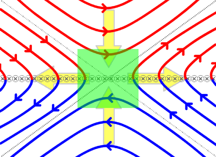
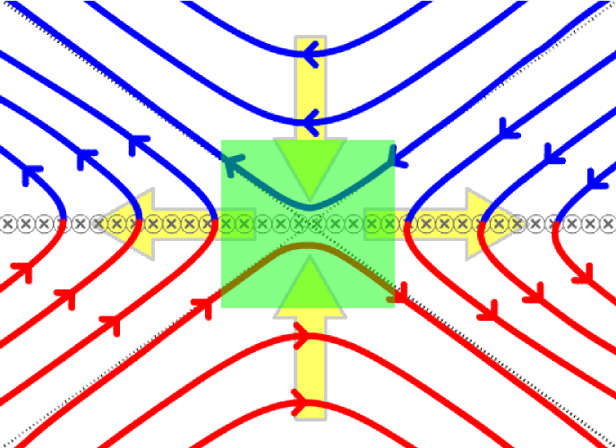
time = 5	time = 6

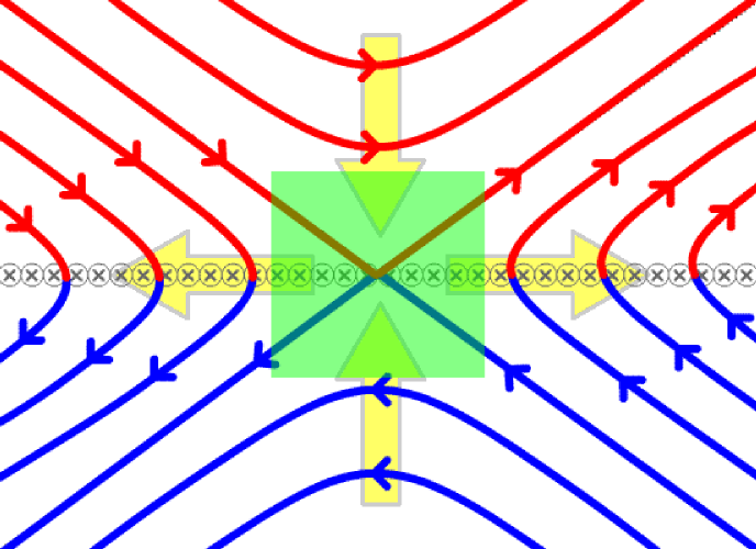
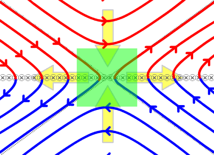
Figure 1: Cartoon of symmetric antiparallel 2D separator reconnection (wikipedia).

At the origin the magnetic field is zero. Symmetry forces physical velocities to be zero at the origin, including the bulk fluid velocity, the fluid velocity of each species, and any flux-transporting flow. The magnetic field lines which intersect the origin are called separatrices and partition the domain into four regions. In an ideal plasma model the separatrices would be frozen in the fluid and therefore it would be impossible to transfer flux across the separatrices. The reconnected flux is defined to be the amount of flux transferred from one region to another. The green rectangle at the center signifies the diffusion region. The ratio of its long side to its short side is called its aspect ratio.  

A definition of magnetic reconnection in general geometry requires a covariant (relativistic) description of the electromagnetic field [HornigSchindler96]. Since this dissertation only studies 2D problems symmetric under 180-degree rotation in the plane about the origin, it defines magnetic reconnection only for this case; the rate of reconnection turns out simply to be the out-of-plane electric field component at the origin, as argued in section LABEL:2DmagneticReconnection.

1.4 Fast magnetic reconnection

1.4.1 Background

Magnetic reconnection is ultimately controlled by Faraday’s evolution equation for the magnetic field,

$$\partial_{t}\color[rgb]{0,0,0}\mathbf{B}+\nabla\times\color[rgb]{0,0,0}\mathbf{E}=0;$$

so the evolution of magnetic field $\color[rgb]{0,0,0}\mathbf{B}$ is determined by the electric field $\color[rgb]{0,0,0}\mathbf{E}$. Plasma physics studies the evolution of plasmas on time scales larger than the plasma period $\lx@glossaries@gls@link{symbol}{plasmafreq}{\leavevmode\omega_{p}}^{-1}$ (the time of oscillation in response to charge separation) and larger than the Debye length $\lambda_{D}$ (the distance traveled by an electron in a plasma period moving at the thermal velocity $v_{ts}$, which is the distance over which charge shielding occurs) [HW04]. On these scales the assumption of quasineutrality holds and Ohm’s law (LABEL:OhmsLawFullTerms) for the electric field applies. For a plasma consisting of electrons and ions, Ohm’s law is

$$\color[rgb]{0,0,0}\mathbf{E}= \color[rgb]{0,0,0}\mathbf{B}\times{\color[rgb]{0,0,0}\mathbf{u}}$$ (ideal term) (1.1)

$$+\color[rgb]{0,0,0}\bm{\eta}\color[rgb]{0,0,0}{\,\bm{\cdot}\,}\color[rgb]{0,0,0}\mathbf{J}$$ (resistive term)

$$+\tfrac{\color[rgb]{0,0,0}m_{\mathrm{i}}-\color[rgb]{0,0,0}m_{\mathrm{e}}}{e\color[rgb]{0,0,0}\rho}\color[rgb]{0,0,0}\mathbf{J}\times\color[rgb]{0,0,0}\mathbf{B}$$ (Hall term)

$$+\tfrac{1}{e\color[rgb]{0,0,0}\rho}\color[rgb]{0,0,0}\nabla{\,\bm{\cdot}\,}\left(\color[rgb]{0,0,0}m_{\mathrm{e}}\color[rgb]{0,0,0}\mathbb{P}_{\mathrm{i}}-\color[rgb]{0,0,0}m_{\mathrm{i}}\color[rgb]{0,0,0}\mathbb{P}_{\mathrm{e}}\right)$$ (pressure term)

$$+\tfrac{\color[rgb]{0,0,0}m_{\mathrm{i}}\color[rgb]{0,0,0}m_{\mathrm{e}}}{e^{2}\color[rgb]{0,0,0}\rho}\left[\partial_{t}\color[rgb]{0,0,0}\mathbf{J}+\color[rgb]{0,0,0}\nabla{\,\bm{\cdot}\,}\left({\color[rgb]{0,0,0}\mathbf{u}}\color[rgb]{0,0,0}\mathbf{J}+\color[rgb]{0,0,0}\mathbf{J}{\color[rgb]{0,0,0}\mathbf{u}}-\tfrac{\color[rgb]{0,0,0}m_{\mathrm{i}}-\color[rgb]{0,0,0}m_{\mathrm{e}}}{e\color[rgb]{0,0,0}\rho}\color[rgb]{0,0,0}\mathbf{J}\color[rgb]{0,0,0}\mathbf{J}\right)\right]$$ (inertial term),

where ${\color[rgb]{0,0,0}\mathbf{u}}$ is fluid velocity, $\color[rgb]{0,0,0}\mathbf{J}$ is electrical current density, $\color[rgb]{0,0,0}\rho$ is mass density, and $\color[rgb]{0,0,0}\mathbb{P}_{\mathrm{i}}$ and $\color[rgb]{0,0,0}\mathbb{P}_{\mathrm{e}}$ are the ion and electron pressure tensors; the constants are the ion mass $\color[rgb]{0,0,0}m_{\mathrm{i}}$, the electron mass $\color[rgb]{0,0,0}m_{\mathrm{e}}$, and the magnitude of the charge on an electron, $e$. The resistivity $\color[rgb]{0,0,0}\bm{\eta}$ requires a closure, typically a function of (electron) temperature unless an anomalous resistivity is defined.

This work restricts consideration to problems symmetric under 180-degree rotation, because it allows a simple analysis of the X-point which identifies constraints and requirements for reconnection. As argued in section LABEL:2DmagneticReconnection, at the X-point Ohm’s law reduces to

$$\begin{aligned} \color[rgb]{0,0,0}\mathbf{E}=&\color[rgb]{0,0,0}\bm{\eta}\color[rgb]{0,0,0}{\,\bm{\cdot}\,}\color[rgb]{0,0,0}\mathbf{J}&\hbox{(resistive term)}\\ &+\tfrac{1}{e\color[rgb]{0,0,0}\rho}\color[rgb]{0,0,0}\nabla{\,\bm{\cdot}\,}\left(\color[rgb]{0,0,0}m_{\mathrm{e}}\color[rgb]{0,0,0}\mathbb{P}_{\mathrm{i}}-\color[rgb]{0,0,0}m_{\mathrm{i}}\color[rgb]{0,0,0}\mathbb{P}_{\mathrm{e}}\right)&\hbox{(pressure term)}\\ &+\tfrac{\color[rgb]{0,0,0}m_{\mathrm{i}}\color[rgb]{0,0,0}m_{\mathrm{e}}}{e^{2}\color[rgb]{0,0,0}\rho}\left[\partial_{t}\color[rgb]{0,0,0}\mathbf{J}+\color[rgb]{0,0,0}\nabla{\,\bm{\cdot}\,}\left({\color[rgb]{0,0,0}\mathbf{u}}\color[rgb]{0,0,0}\mathbf{J}+\color[rgb]{0,0,0}\mathbf{J}{\color[rgb]{0,0,0}\mathbf{u}}-\tfrac{\color[rgb]{0,0,0}m_{\mathrm{i}}-\color[rgb]{0,0,0}m_{\mathrm{e}}}{e\color[rgb]{0,0,0}\rho}\color[rgb]{0,0,0}\mathbf{J}\color[rgb]{0,0,0}\mathbf{J}\right)\right]&\hbox{(inertial term)}\end{aligned}$$ (1.2)

where only the out-of-plane component survives. Since the rate of reconnection is the out-of-plane component of the electric field at the origin, this confirms that one of these three terms must be nonzero to support reconnection.

Magnetohydrodynamic (MHD) models of plasma explictly assume a form of Ohm’s law and evolve a system sufficient to determine the quantities it involves. Ideal MHD discards all terms in Ohm’s law except the ideal term and is the simplest model of plasma. In ideal MHD magnetic reconnection is not possible. The next simplest model, resistive MHD, also retains the resistive term. Resistive MHD allows magnetic reconnection to occur, because magnetic field lines can diffuse through the plasma; as we will discuss, steady reconnection rates are slow for resistive MHD unless an anomalous resistivity is used. Resistive Hall MHD includes the Hall term as well, allowing much faster rates of steady reconnection. Models which include terms of Ohm’s law beyond resistive MHD are collectively known as extended MHD models.

1.4.2 Historical background for fast magnetic reconnection

The notion of magnetic reconnection was introduced by Dungey ([dungey53], 1953). In the subsequent decades people attempted to explain reconnection in terms of resistive MHD. Sweet ([Sweet58], 1958) and Parker ([Parker57], 1957) developed a model of steady two-dimensional magnetic reconnection. The Sweet-Parker model assumes that magnetic reconnection occurs in a thin, rectangular diffusion region containing nearly antiparallel magnetic field lines. The aspect ratio of a rectangle denotes the ratio consisting of the length of the long side divided by the length of the short side. In the Sweet-Parker model of reconnection the aspect ratio of the diffusion region is assumed to be large, implying that the magnetic field lines have a “Y-type” configuration. Plasma is assumed to flow slowly into the broad sides of the rectangle and rapidly out of the narrow sides of the rectangle. In the diffusion region, gradients in the magnetic field result in diffusion of the magnetic field (and hence slipping of magnetic field lines through the plasma) and a sheet of electrical current. Using this model, Parker ([Parker63], 1963) estimated a typical rate of magnetic reconnection in solar flares based on Spitzer’s formula for resistivity (which is based on Coulomb collisions and asserts that resistivity is a function of temperature, see [Spitzer62]) and found that the predicted rate of reconnection was at least one hundred times too small to account for observed solar flare time scales.

The essential impediment to fast reconnection in the Sweet-Parker model is the tension between the need for a narrow diffusion region (so that magnetic field gradients can be sufficiently strong) and a wide diffusion region (so that plasma can flow out of the narrow sides of the rectangle rapidly enough). Subsequent models of steady reconnection obtained faster rates of reconnection by assuming anomalously high values of resistivity in the diffusion region and/or by assuming an “X-type” magnetic field configuration (in particular a diffusion region with a small aspect ratio) which allows strong magnetic field gradients at the X-point while opening up the outflow so that it is not throttled by being confined to a narrow rectangle [priestForbes00]. The first such model was devised by Petschek ([petschek64], 1964) and consisted of an X-type magnetic field geometry with a miniature Sweet-Parker region at the center. The Petschek model allowed much faster reconnection rates than the Sweet-Parker model, and thus Sweet-Parker reconnection became designated as slow reconnection while reconnection rates on the order given by the Petschek model were identified as fast reconnection.

When numerical simulation of magnetic reconnection became feasible, it was found that magnetic reconnection resulted in Y-type configurations and slow reconnection if a uniform resistivity was assumed, whereas X-type configurations and fast reconnection occurred if anomalously high values of resistivity were assumed near the X-point [birnPriest07]. There are physical reasons to expect anomalously high values of resistivity near the X-point. First, resistive drag may depend nonlinearly on electric current. Electrical currents are strong in the reconnection region. Electrical currents represent relative drift of ions and electrons. If this relative drift becomes strong enough, a streaming instability develops, limiting interspecies drift and greatly increasing resistivity. Second, resistivity may be spatially dependent in a weakly collisional plasma where fluid closures cannot be rigorously justified. Spitzer’s formula for resistivity assumes collisional transport theory, which is applicable when the mean free path of a particle is small relative to the length scale of variations in the magnetic field and gas-dynamic quantities. Particle mean free paths are much larger than the width of current sheets or diffusion layers where reconnection occurs, and so collisional transport theory is not applicable even when, as in the solar corona, it is applicable to large-scale structures (see [priestForbes00], page 45); thus, the reconnection region is governed by collisionless physics in essentially all space and laboratory plasmas where magnetic reconnection is important [brackbill:priv11].

Thus, for resistive MHD the game of modeling reconnection naturally became to determine anomalous values of resistivity that account for fast reconnection. By assuming a spatially dependent anomalous resistivity one can essentially prescribe a desired rate of reconnection. Some space modelers have taken the approach of prescribing spatially anomalous resistivities which give results that seem to agree with observational and statistical data. Such an approach can be effective in a specific problem domain such as space weather modeling, but in general we prefer the simplest models with the greatest explanatory and predictive success, which are based in physical principles, and which give physical insight.

One can obtain fast rates of reconnection using an anomalous resistivity that is dependent on current but spatially independent. The project to formulate a spatially independent anomalous resistivity that accurately models reconnection has fallen short, however, on two accounts. First, there are many formulas for anomalous resisivity, and a simple basis for these formulas has been elusive [satoHayashi79, article:Vasyliunas75, brackbill:priv11]. Second, in weakly collisional regimes steady reconnection is supported primarily by the divergence of the species pressure tensors rather than by resistive drag, and therefore attempting to attribute the reconnection electric field to a resistive term is artificial and does not promise to give physical insight; the end road of insisting on an anomalous resistivity framework is that an appropriate formula for the anomalous resistivity will probably be found to be in terms of the divergence of the electron pressure tensor!

Although a uniform resistivity results in a long, thin current sheet and slow reconnection, this configuration is often unstable. Furth, Killeen, and Rosenbluth ([furth63], 1963) found that a current sheet with an aspect ratio of about $2\pi$ or greater is unstable to spontaneous reconnection which forms magnetic islands. This process is called the tearing mode instability, and the magnetic islands are referred to as plasmoids. Bulanov et al. ([bulanov78], 1978) repeated the tearing mode calculation of [furth63] assuming linear outflow along the current sheet and found that the outflow had a stabilizing effect.

Jumping forward to the past decade, Loureiro, Schekochihin, and Cowley (2007, [article:LouSchCow07]) performed an asympototic analysis in the inverse of the aspect ratio of the current sheet and showed that for a current sheet of sufficiently large length $L$ (for which the Lundquist number $\mathrm{Lu}:=L\color[rgb]{0,0,0}v_{A}/\color[rgb]{0,0,0}\eta$ is greater than a critical value of about $4\times 10^{4}$, corresponding to an aspect ratio of about 200; see [huangBh10]), a chain of plasmoids rapidly forms. Subsequent simulations have confirmed that the ejection of these plasmoids allows fast reconnection rates even in resistive MHD. The consequence is that although resistive MHD with uniform resistivity does not admit fast reconnection, for sufficiently large (e.g. astrophysical) domains statistically steady fast reconnection can be expected via the cascading formation and ejection of plasmoids [huangBh10]. Nevertheless, one can still make the categorical assertion that resistive MHD with uniform resistivity does not support steady-state fast reconnection.

In laboratory plasmas Lundquist numbers are typically on the order of $10^{3}$ (page 44 in [priestForbes00]), which is too small to give rise to plasmoid-mediated reconnection; instead one expects (slow) Sweet-Parker reconnection if the ion inertial length δs is larger than the Sweet-Parker layer thickness. For ion skin depth smaller than the Sweet-Parker layer thickness one expects fast, Hall-mediated reconnection instead, as discussed in the next section. (See p315 in [zweibel09] and Figure 1 in [huang10].)

1.4.3 The GEM problem

The inadequacy of resistive MHD to account for reconnection electric fields in the diffusion region lead to studies of reconnection using using extended MHD. The historical development of these studies is traced in [shay01], and lead to the following observations regarding 2D separator reconnection. As shown for collisional tearing in [Terasawa83], the Hall current effect becomes important for a current sheet whose width is comparable to the ion inertial length. Outside of the current sheet gradients are small, and the ideal term dominates in Ohm’s law. Within the current sheet the Hall term becomes significant and the ions decouple from the magnetic field lines, defining the ion diffusion region. In a smaller region the electron pressure term (or inertial term) becomes significant and the electrons decouple from the magnetic field as well, defining the electron diffusion region.

The culmination of these studies and observations was the formulation and simulation of the Geospace Environmental Modeling magnetic reconnection challenge problem (GEM problem) in 2001 [article:GEM]. The GEM problem was formulated to study the ability of plasma models to resolve fast magnetic reconnection [article:GEM]. The GEM problem identified two-fluid/Hall effects as critical to allow fast reconnection. Although ideal Hall MHD does not admit reconnection, resistive Hall MHD (even with small resistivity) was found to admit fast reconnection [shay01], as if the Hall term were a catalyst accelerating the must slower rate of reconnection that occurs in resistive MHD without the Hall term.

I remark that ideal Hall MHD (Ohm’s law using only the ideal term and the Hall term) does not allow reconnection because a flux-transporting flow exists; magnetic field lines are essentially frozen to the electrons. The ideal Hall MHD simulations in [shay01] were able to get fast reconnection rates because of the presence of numerical resistivity; the results therefore cannot be converged. Finding 3 at the end of section 1 suggests that in their simulations reconnection is supported by numerical resistivity with an anomalously high value near the X-point. It appears that it is still an open question whether converged fast reconnection is possible in resistive Hall MHD with uniform resistivity. If the answer is no, then one may conclude that short of anomalous closures nonzero divergence of the pressure tensor is necessary for converged steady fast magnetic reconnection. This suggests a study of of reconnection with a two-fluid model with resistivity but without viscosity, with and without the inertial term.

Pair plasma GEM simulations

Since the seminal GEM problem studies had identified the Hall effect as the essential physics to admit fast reconnection, it was natural to investigate reconnection rates in pair plasmas, for which $\color[rgb]{0,0,0}m_{\mathrm{e}}=\color[rgb]{0,0,0}m_{\mathrm{i}}$ and the Hall term of Ohm’s law is absent. Particle simulations by Bessho and Bhattacharjee of antiparallel reconnection [article:BeBh05, article:BeBh07, bessho10] have demonstrated that fast reconnection rates occur even in the case of pair plasmas; they find that the divergence of the pressure tensor is the term of equation (1.2) that primarily supports the reconnection electric field. For the guide-field case, in which the out-of-plane component of the magnetic field at the origin is nonzero, Chacón et al. [article:ChSiLuZo08] subsequently demonstrated that steady fast reconnection is possible in a viscous incompressible model of pair plasma if viscosity dominates but not if resistivity dominates.

In this work we simulate the pair plasma version of the GEM problem with a two-fluid adiabatic model without resistivity and show that rates of reconnection are still fast (although our rate of reconnection is only 60% of the rate in the PIC simulations reported e.g. in [article:BeBh07]).

Two-fluid GEM simulations

The fluid models used in the seminal GEM problem studies did not include the pressure and inertial terms of Ohm’s law. It is therefore natural to ask whether the inclusion of these terms would allow significantly improved agreement of fluid simulation of magnetic reconnection with kinetic simulations.

In 2005 Hakim, Loverich, and Shumlak simulated fast magnetic reconnection with an adiabatic inviscid five-moment two-fluid Maxwell model model which implies an Ohm’s law that includes the Hall term, the inertial term, and a pressure term with scalar pressures [article:HaLoSh06]. Their figure 10 shows their reconnected flux values superimposed on the reconnection rates reported in the seminal GEM problem papers and arguably shows improved agreement with particle simulations in comparison to the Hall MHD simulations. In 2007 Hakim submitted simulations of the GEM problem with a two-fluid Maxwell model which uses a hyperbolic (adiabatic inviscid) five-moment model for the electrons and a hyperbolic model for the ions and again obtained reconnection rates that agree well with kinetic simulations [article:Hakim08].

The models used by Loverich, Hakim, and Shumlak are hyperbolic. In particular, for the electrons they use hyperbolic five-moment gas dynamics, which uses truncation closures for the deviatoric pressure and heat flux. As a proxy for Ohm’s law (1.1) one may consider the electron momentum equation (LABEL:momentumEvolution) solved for the electric field:

$$\begin{aligned} \color[rgb]{0,0,0}\mathbf{E}&=\color[rgb]{0,0,0}\mathbf{B}\times{\color[rgb]{0,0,0}\mathbf{u}}_{\mathrm{e}}&\hbox{(ideal term)}\\ &+\frac{-\color[rgb]{0,0,0}\mathbf{R}_{\mathrm{e}}}{q_{\mathrm{e}}\color[rgb]{0,0,0}n_{\mathrm{e}}}&\hbox{(resistive term)}\\ &+\frac{\color[rgb]{0,0,0}\nabla{\,\bm{\cdot}\,}\color[rgb]{0,0,0}\mathbb{P}_{\mathrm{e}}}{q_{\mathrm{e}}\color[rgb]{0,0,0}n_{\mathrm{e}}}&\hbox{(pressure term)}\\ &+\frac{m_{\mathrm{e}}}{q_{\mathrm{e}}}d_{t}{\color[rgb]{0,0,0}\mathbf{u}}_{\mathrm{e}}&\hbox{(inertial term)}.\end{aligned}$$ (1.3)

At the X-point symmetry the ideal term disappears, simplifying this to the equivalent of equation (1.2). In the simulations of Loverich, Hakim, and Shumlak the resistive term is zero and the pressure term vanishes at the X-point because the deviatoric pressure is zero. This would force the electron velocity at the X-point to ramp with reconnected flux. As our simulations indicate (see figure LABEL:fig:0), this almost certainly is not realized in their simulations for later times, and therefore their solutions are presumably not converged for later times. Furthermore, based on kinetic simulations (see e.g. figure LABEL:fig:6), we expect the pressure term to dominate at the X-point.

We were therefore motivated to consider two-fluid model with viscosity in both species fluids. An easy way to implement viscosity in a gas is to represent it using a ten-moment model (also known as a Gaussian-moment model with relaxation to isotropy. A ten-moment model with relaxation to isotropy agrees with a viscous five-moment model for fast isotropization rates and small pressure anisotropies. For slow isotropization rates, large pressure anisotropies can develop. In kinetic simulations, strong pressure anisotropy is in fact observed at the X-point (see figure 6 of [article:SmGr06]), adding to our motivation for use of a ten-moment isotropizing model for both electrons and ions rather than a five-moment viscous model.

Using the ten-moment two-fluid model to simulate the GEM problem, we obtain qualitatively good agreement with kinetic simulations for plots of the pressure tensor at the time of peak reconnection rate (roughly 16–18, where the unit of time is a typical ion angular gyroperiod as defined in the GEM problem); at this time the pressure is highly agyrotropic in the immediate vicinity of reconnection point. In the approximate time interval from 18 to 28 the rate of reconnection remains approximately constant while the electron temperature tensor becomes increasingly singular near the X-point. For a coarse mesh this temperature singularity does not interfere with the normal progression and saturation of reconnection, probably due to numerical thermal diffusion, but when the mesh is refined the singularity becomes sharp and ultimately prevents normal progression of reconnection. The specific terminating behavior is erratic and hard to predict, but in general at the X-point the temperature parallel to the outflow axis will become very cold while the temperature parallel to the inflow axis will become very hot. Unless positivity limiters are applied the simulation crashes when a non-positive-definite temperature tensor develops. (Typically the anisotropically hot spot at the origin splits into two hot spots along the outflow axis before this crash occurs.) If positivity limiters are applied then a secondary island at the origin is likely to form. If symmetry is enforced then this stops reconnection, but if not then spontaneous symmetry-breaking can eject the island and allow reconnection to proceed.

1.4.4 Entropy production and heat flux requirements for steady magnetic reconnection

The characteristic behavior of dynamical systems turns critically on the character of their equilibria. To understand the difficulties encountered with the GEM problem when an adiabatic model is used, we consider the entropy production and heat flux requirements for steady magnetic reconnection. We show that for models which lack a mechanism for heat flux, in reconnection problems that are symmetric under 180-degree rotation about the origin (as holds for the GEM problem), solutions which exhibit steady reconnection must be singular.

1.4.5 Gyrotropic ten-moment heat flux closure

We therefore consider what an appropriate 10-moment heat flux closure would be. In the presence of a magnetic field appropriate diffusive closures need to be gyrotropic rather than isotropic. We therefore generalize the isotropic ten-moment heat flux closure recently formulated by McDonald and Groth to the gyrotropic case.

1.5 Model equations

For subsequent reference, in this section we list the systems of equations that define the models discussed in this work. All simulations have been performed using the 10-moment two-fluid Maxwell model or the 5-moment two-fluid Maxwell model.

The relationship among models is laid out in figure 2. As the standard of truth we take the Boltzmann-Maxwell model displayed in figure 3. The 10-moment two-fluid Maxwell equations that we solve are displayed in figure 4. The 5-moment two-fluid Maxwell equations that we solve are displayed in figure LABEL:fig:5mom2fluidMaxwell. Taking the light speed to infinity converts the two-fluid Maxwell models to MHD models. In solving the two-fluid Maxwell equations our goal is to approximate the MHD systems, which we attempt to do by using a sufficiently high light speed. We therefore display the equations of 10-moment 2-fluid MHD in figure LABEL:fig:10mom2fluidMHD and display the equations of 5-moment 2-fluid MHD in figure LABEL:fig:5mom2fluidMHD. This work calculates intraspecies collisional closure coefficients using a Chapman-Enskog expansion with a Gaussian-BGK collision operator. The resulting formulas for closure coefficients are displayed for the ten-moment model in figure LABEL:fig:10momCoef and for the five-moment model in figure LABEL:fig:5momCoef.

 Model hierarchy

$$\begin{CD}\hbox{(two-fluid Boltzmann-Maxwell)}\\ @V{}V{}V\\ \hbox{(10-moment two-fluid Maxwell)}@>{}>{}>\hbox{(10-moment two-fluid MHD)}\\ @V{}V{}V@V{}V{}V\\ \hbox{(5-moment two-fluid Maxwell)}@>{}>{}>\hbox{(5-moment two-fluid MHD)}\\ @V{}V{}V\\ \hbox{(5-moment MHD)}\\ \end{CD}$$

Figure 2: Hierarchy of models considered in this work.

Motion down and to the right indicates use of simplifying limits. Motion down reduces the number of moments evolved. Motion to the right takes light speed to infinity.  

 Boltzmann-Maxwell model

• Kinetic/Boltzmann equations:

  $$\partial_{t}\color[rgb]{0,0,0}f_{\mathrm{i}} +{\color[rgb]{0,0,0}\mathbf{v}}\color[rgb]{0,0,0}{\,\bm{\cdot}\,}\color[rgb]{0,0,0}\nabla_{{\color[rgb]{0,0,0}\mathbf{x}}}\color[rgb]{0,0,0}f_{\mathrm{i}} +\color[rgb]{0,0,0}\mathbf{a}_{\mathrm{i}}\color[rgb]{0,0,0}{\,\bm{\cdot}\,}\nabla_{{\color[rgb]{0,0,0}\mathbf{v}}}\color[rgb]{0,0,0}f_{\mathrm{i}} =\color[rgb]{0,0.10,0.60}C_{\mathrm{i}} +\color[rgb]{1,0,1}C_{\mathrm{i}\mathrm{e}}$$

  $$\partial_{t}\color[rgb]{0,0,0}f_{\mathrm{e}} +{\color[rgb]{0,0,0}\mathbf{v}}\color[rgb]{0,0,0}{\,\bm{\cdot}\,}\color[rgb]{0,0,0}\nabla_{{\color[rgb]{0,0,0}\mathbf{x}}}\color[rgb]{0,0,0}f_{\mathrm{e}} +\color[rgb]{0,0,0}\mathbf{a}_{\mathrm{e}}\color[rgb]{0,0,0}{\,\bm{\cdot}\,}\nabla_{{\color[rgb]{0,0,0}\mathbf{v}}}\color[rgb]{0,0,0}f_{\mathrm{e}} =\color[rgb]{0,0.10,0.60}C_{\mathrm{e}} +\color[rgb]{1,0,1}C_{\mathrm{e}\mathrm{i}}$$

• Maxwell’s equations:

  $$\partial_{t}\color[rgb]{0,0,0}\mathbf{B}+\nabla\times\color[rgb]{0,0,0}\mathbf{E}=0, \color[rgb]{0,0,0}\nabla\color[rgb]{0,0,0}{\,\bm{\cdot}\,}\color[rgb]{0,0,0}\mathbf{B}=0$$

  $$\partial_{t}\color[rgb]{0,0,0}\mathbf{E}-c^{2}\nabla\times\color[rgb]{0,0,0}\mathbf{B}=-\color[rgb]{0,0,0}\mathbf{J}/\epsilon_{0}, \color[rgb]{0,0,0}\nabla\color[rgb]{0,0,0}{\,\bm{\cdot}\,}\color[rgb]{0,0,0}\mathbf{E}=\color[rgb]{0,0,0}\sigma/\epsilon_{0}$$

• Definitions:

  $$\color[rgb]{0,0,0}\sigma:=\sum_{\mathrm{s}}\frac{q_{\mathrm{s}}}{m_{\mathrm{s}}}\int\color[rgb]{0,0,0}f_{\mathrm{s}}\,d{\color[rgb]{0,0,0}\mathbf{v}},$$

  $$\color[rgb]{0,0,0}\mathbf{J}:=\sum_{\mathrm{s}}\frac{q_{\mathrm{s}}}{m_{\mathrm{s}}}\int{\color[rgb]{0,0,0}\mathbf{v}}\color[rgb]{0,0,0}f_{\mathrm{s}}\,d{\color[rgb]{0,0,0}\mathbf{v}}$$

  $$\begin{aligned} \color[rgb]{0,0,0}\mathbf{a}_{\mathrm{i}}&:=\tfrac{e}{m_{i}}&&\left(\color[rgb]{0,0,0}\mathbf{E}+{\color[rgb]{0,0,0}\mathbf{v}}\times\color[rgb]{0,0,0}\mathbf{B}\right),\\ \color[rgb]{0,0,0}\mathbf{a}_{\mathrm{e}}&:=\tfrac{-e}{m_{e}}&&\left(\color[rgb]{0,0,0}\mathbf{E}+{\color[rgb]{0,0,0}\mathbf{v}}\times\color[rgb]{0,0,0}\mathbf{B}\right)\end{aligned}$$

Figure 3: Equations of the two-species Boltzmann-Maxwell model (standard of truth).

The interspecies collision operators ${\color[rgb]{1,0,1}C_{ie}}$ and ${\color[rgb]{1,0,1}C_{ei}}$ are generally ignored in this work, but the intraspecies collision operators ${\color[rgb]{0,0.10,0.60}C_{i}}$ and ${\color[rgb]{0,0.10,0.60}C_{e}}$ play a critical role.  

 Ten-moment two-fluid Maxwell model

Gas dynamics equations

$$\mspace{-30.0mu}\color[rgb]{0,0,0}\overline{\delta}_{t}^{\mathrm{i}}\begin{bmatrix}\color[rgb]{0,0,0}\rho_{\mathrm{i}}\\ \color[rgb]{0,0,0}\rho_{\mathrm{i}}{\color[rgb]{0,0,0}\mathbf{u}}_{\mathrm{i}}\\ \color[rgb]{0,0,0}\rho_{\mathrm{i}}\color[rgb]{0,0,0}\mathbbm{e}_{\mathrm{i}}\end{bmatrix} +\begin{bmatrix}0\\ \color[rgb]{0,0,0}\nabla{\,\bm{\cdot}\,}\color[rgb]{0,0,0}\mathbb{P}_{\mathrm{i}}\\ \operatorname{Sym2}(\color[rgb]{0,0,0}\nabla{\,\bm{\cdot}\,}(\color[rgb]{0,0,0}\mathbb{P}_{\mathrm{i}}{\color[rgb]{0,0,0}\mathbf{u}}_{\mathrm{i}}))+\lx@glossaries@gls@link{symbol}{qT}{\leavevmode{\color[rgb]{1,0,0}\nabla{\,\bm{\cdot}\,}\bm{\mathbbm{q}}_{\mathrm{i}}}}\end{bmatrix} =\color[rgb]{0,0,0}\sigma_{\mathrm{i}}\begin{bmatrix}0\\ \color[rgb]{0,0,0}\mathbf{E}+{\color[rgb]{0,0,0}\mathbf{u}}_{\mathrm{i}}\times\color[rgb]{0,0,0}\mathbf{B}\\ {\operatorname{Sym2}({\color[rgb]{0,0,0}\mathbf{u}}_{\mathrm{i}}\color[rgb]{0,0,0}\mathbf{E}+\color[rgb]{0,0,0}\mathbbm{e}_{\mathrm{i}}\times\color[rgb]{0,0,0}\mathbf{B})}\end{bmatrix} +\begin{bmatrix}0\\ \lx@glossaries@gls@link{symbol}{R}{\leavevmode{\color[rgb]{1,0,1}\mathbf{R}_{\mathrm{i}}}}\\ \lx@glossaries@gls@link{symbol}{RT}{\leavevmode{\color[rgb]{0,0.10,0.60}{\mathbb{R}}_{\mathrm{i}}}}+\lx@glossaries@gls@link{symbol}{Q}{\leavevmode{\color[rgb]{1,0,1}\mathbb{Q}_{\mathrm{i}}}}\end{bmatrix}$$

$$\mspace{-30.0mu}\color[rgb]{0,0,0}\overline{\delta}_{t}^{\mathrm{e}}\begin{bmatrix}\color[rgb]{0,0,0}\rho_{\mathrm{e}}\\ \color[rgb]{0,0,0}\rho_{\mathrm{e}}{\color[rgb]{0,0,0}\mathbf{u}}_{\mathrm{e}}\\ \color[rgb]{0,0,0}\rho_{\mathrm{e}}\color[rgb]{0,0,0}\mathbbm{e}_{\mathrm{e}}\end{bmatrix} +\begin{bmatrix}0\\ \color[rgb]{0,0,0}\nabla{\,\bm{\cdot}\,}\color[rgb]{0,0,0}\mathbb{P}_{\mathrm{e}}\\ \operatorname{Sym2}(\color[rgb]{0,0,0}\nabla{\,\bm{\cdot}\,}(\color[rgb]{0,0,0}\mathbb{P}_{\mathrm{e}}{\color[rgb]{0,0,0}\mathbf{u}}_{\mathrm{e}}))+\lx@glossaries@gls@link{symbol}{qT}{\leavevmode{\color[rgb]{1,0,0}\nabla{\,\bm{\cdot}\,}\bm{\mathbbm{q}}_{\mathrm{e}}}}\end{bmatrix} =\color[rgb]{0,0,0}\sigma_{\mathrm{e}}\begin{bmatrix}0\\ \color[rgb]{0,0,0}\mathbf{E}+{\color[rgb]{0,0,0}\mathbf{u}}_{\mathrm{e}}\times\color[rgb]{0,0,0}\mathbf{B}\\ {\operatorname{Sym2}({\color[rgb]{0,0,0}\mathbf{u}}_{\mathrm{e}}\color[rgb]{0,0,0}\mathbf{E}+\color[rgb]{0,0,0}\mathbbm{e}_{\mathrm{e}}\times\color[rgb]{0,0,0}\mathbf{B})}\end{bmatrix} +\begin{bmatrix}0\\ \lx@glossaries@gls@link{symbol}{R}{\leavevmode{\color[rgb]{1,0,1}\mathbf{R}_{\mathrm{e}}}}\\ \lx@glossaries@gls@link{symbol}{RT}{\leavevmode{\color[rgb]{0,0.10,0.60}{\mathbb{R}}_{\mathrm{e}}}}+\lx@glossaries@gls@link{symbol}{Q}{\leavevmode{\color[rgb]{1,0,1}\mathbb{Q}_{\mathrm{e}}}}\end{bmatrix}$$

Maxwell’s equations:

$$\partial_{t}\color[rgb]{0,0,0}\mathbf{B}+\nabla\times\color[rgb]{0,0,0}\mathbf{E}=0, \color[rgb]{0,0,0}\nabla\color[rgb]{0,0,0}{\,\bm{\cdot}\,}\color[rgb]{0,0,0}\mathbf{B}=0$$

$$\partial_{t}\color[rgb]{0,0,0}\mathbf{E}-c^{2}\nabla\times\color[rgb]{0,0,0}\mathbf{B}=-\color[rgb]{0,0,0}\mathbf{J}/\epsilon_{0}, \color[rgb]{0,0,0}\nabla\color[rgb]{0,0,0}{\,\bm{\cdot}\,}\color[rgb]{0,0,0}\mathbf{E}=\color[rgb]{0,0,0}\sigma/\epsilon_{0}$$

Definitions:

$$\mspace{-30.0mu}\color[rgb]{0,0,0}\sigma_{\mathrm{i}}=en_{\mathrm{i}},\quad\color[rgb]{0,0,0}\sigma_{\mathrm{e}}=-en_{\mathrm{e}},\quad\color[rgb]{0,0,0}\sigma=\color[rgb]{0,0,0}\sigma_{\mathrm{i}}+\color[rgb]{0,0,0}\sigma_{\mathrm{e}}$$

$$\mspace{-30.0mu}\color[rgb]{0,0,0}\mathbf{J}=\color[rgb]{0,0,0}\sigma_{\mathrm{i}}{\color[rgb]{0,0,0}\mathbf{u}}_{\mathrm{i}}+\color[rgb]{0,0,0}\sigma_{\mathrm{e}}{\color[rgb]{0,0,0}\mathbf{u}}_{\mathrm{e}}$$

$$\mspace{-30.0mu}\lx@glossaries@gls@link{symbol}{dcs}{\leavevmode\overline{\delta}_{t}^{s}}\alpha:=\partial_{t}\alpha+\color[rgb]{0,0,0}\nabla{\,\bm{\cdot}\,}({\color[rgb]{0,0,0}\mathbf{u}}_{\mathrm{s}}\alpha)$$

Closures:

$$\vspace{-1ex}\lx@glossaries@gls@link{symbol}{RT}{\leavevmode{\color[rgb]{0,0.10,0.60}{\mathbb{R}}_{\mathrm{s}}}}=-\color[rgb]{0,0,0}\tau_{\mathrm{s}}^{-1}\color[rgb]{0,0,0}\mathbb{P}^{\circ}_{\mathrm{s}}$$

$$\lx@glossaries@gls@link{symbol}{qT}{\leavevmode{\color[rgb]{1,0,0}\bm{\mathbbm{q}}_{\mathrm{s}}}}=-\tfrac{2}{5}\color[rgb]{0,0,0}\bm{K}_{\mathrm{s}}\color[rgb]{0,0,0}\mathrel{\vbox{\offinterlineskip\hbox{$\bm{\cdot}$}\vskip-1.50696pt\hbox{$\bm{\cdot}$}\vskip-1.50696pt\hbox{$\bm{\cdot}$}}}\operatorname{Sym3}\left(\color[rgb]{0,0,0}{\bm{\pi}}_{\mathrm{s}}\color[rgb]{0,0,0}{\,\bm{\cdot}\,}\color[rgb]{0,0,0}\nabla\color[rgb]{0,0,0}\mathbb{T}_{\mathrm{s}}\right)$$

$$\lx@glossaries@gls@link{symbol}{R}{\leavevmode{\color[rgb]{1,0,1}\mathbf{R}_{\mathrm{i}}}}=-\lx@glossaries@gls@link{symbol}{R}{\leavevmode{\color[rgb]{1,0,1}\mathbf{R}_{\mathrm{e}}}}=\color[rgb]{0,0,0}\sigma_{\mathrm{i}}\color[rgb]{0,0,0}\sigma_{\mathrm{e}}\lx@glossaries@gls@link{symbol}{Tresistivity}{\leavevmode{\color[rgb]{1,0,1}\bm{\eta}}}\color[rgb]{0,0,0}{\,\bm{\cdot}\,}({\color[rgb]{0,0,0}\mathbf{u}}_{\mathrm{e}}-{\color[rgb]{0,0,0}\mathbf{u}}_{\mathrm{i}})$$

$$\lx@glossaries@gls@link{symbol}{Q}{\leavevmode{\color[rgb]{1,0,1}\mathbb{Q}_{\mathrm{s}}}}=?\lx@glossaries@gls@link{symbol}{QTf}{\leavevmode{\color[rgb]{1,0,1}\mathbb{Q}^{f}_{\mathrm{s}}}}+\lx@glossaries@gls@link{symbol}{QTt}{\leavevmode{\color[rgb]{1,0,1}\mathbb{Q}^{t}_{\mathrm{s}}}}?$$

$$\lx@glossaries@gls@link{symbol}{QTf}{\leavevmode{\color[rgb]{1,0,1}\mathbb{Q}^{f}_{\mathrm{e}}}}=\frac{m_{\mathrm{i}}}{m_{\mathrm{i}}+m_{\mathrm{e}}}\operatorname{Sym2}\left((\alpha^{\color[rgb]{0,0,0}\parallel}_{\mathrm{e}}-\alpha^{\perp}_{\mathrm{e}})\lx@glossaries@gls@link{symbol}{R}{\leavevmode{\color[rgb]{1,0,1}\mathbf{R}_{\mathrm{i}}}}{\color[rgb]{0,0,0}\mathbf{w}}_{\mathrm{e}}+\alpha^{\perp}_{\mathrm{e}}\lx@glossaries@gls@link{symbol}{R}{\leavevmode{\color[rgb]{1,0,1}\mathbf{R}_{\mathrm{i}}}}\color[rgb]{0,0,0}{\,\bm{\cdot}\,}{\color[rgb]{0,0,0}\mathbf{w}}_{\mathrm{e}}\operatorname{{\bm{\mathbbm{1}}}}\right)\,?$$

$$\lx@glossaries@gls@link{symbol}{QTt}{\leavevmode{\color[rgb]{1,0,1}\mathbb{Q}^{t}_{\mathrm{e}}}}=\tfrac{2}{3}{\color[rgb]{1,0,1}K_{\mathrm{e}\mathrm{i}}}n_{\mathrm{e}}n_{\mathrm{i}}\left(\color[rgb]{0,0,0}\mathbb{T}_{\mathrm{i}}-\color[rgb]{0,0,0}\mathbb{T}_{\mathrm{e}}\right)?$$

Figure 4: Equations of the 10-moment 2-fluid Maxwell model.

The interspecies collisional terms ${\color[rgb]{1,0,1}\mathbf{R}_{\mathrm{s}}}$ and ${\color[rgb]{1,0,1}\mathbb{Q}_{\mathrm{s}}}$ are generally ignored in this work. The intraspecies collisional terms ${\color[rgb]{0,0.10,0.60}{\mathbb{R}}_{\mathrm{s}}}$ are used in the simulations and play a critical role; we study reconnection as the isotropization rates $\color[rgb]{0,0,0}\tau_{\mathrm{s}}$ are dialed between $0$ and $\infty$. The simulations neglect ${\color[rgb]{1,0,0}\bm{\mathbbm{q}}_{\mathrm{s}}}$, evidently causing late-time singularities.  

 Five-moment two-fluid Maxwell model

Gas dynamics equations

$$\mspace{-30.0mu}\color[rgb]{0,0,0}\overline{\delta}_{t}^{\mathrm{i}}\begin{bmatrix}\color[rgb]{0,0,0}\rho_{\mathrm{i}}\\ \color[rgb]{0,0,0}\rho_{\mathrm{i}}{\color[rgb]{0,0,0}\mathbf{u}}_{\mathrm{i}}\\ \color[rgb]{0,0,0}\rho_{\mathrm{i}}\color[rgb]{0,0,0}\mathrm{e}_{\mathrm{i}}\end{bmatrix} +\begin{bmatrix}0\\ \color[rgb]{0,0,0}\nabla p_{\mathrm{i}}+\lx@glossaries@gls@link{symbol}{dPT}{\leavevmode{\color[rgb]{1,0,0}\nabla{\,\bm{\cdot}\,}\mathbb{P}^{\circ}_{\mathrm{i}}}}\\ {\color[rgb]{0,0,0}\nabla{\,\bm{\cdot}\,}({\color[rgb]{0,0,0}\mathbf{u}}_{\mathrm{i}}p_{\mathrm{i}})+{\color[rgb]{1,0,0}\nabla{\,\bm{\cdot}\,}(\mathbf{u}_{\mathrm{i}}{\,\bm{\cdot}\,}\mathbb{P}^{\circ}_{\mathrm{i}})}+\lx@glossaries@gls@link{symbol}{qT}{\leavevmode{\color[rgb]{1,0,0}\nabla{\,\bm{\cdot}\,}\bm{\mathbbm{q}}_{\mathrm{i}}}}}\end{bmatrix} =\color[rgb]{0,0,0}\sigma_{\mathrm{i}}\begin{bmatrix}0\\ \color[rgb]{0,0,0}\mathbf{E}+{\color[rgb]{0,0,0}\mathbf{u}}_{\mathrm{i}}\times\color[rgb]{0,0,0}\mathbf{B}\\ {{\color[rgb]{0,0,0}\mathbf{u}}_{\mathrm{i}}\color[rgb]{0,0,0}{\,\bm{\cdot}\,}\color[rgb]{0,0,0}\mathbf{E}}\end{bmatrix} +\begin{bmatrix}0\\ {\color[rgb]{1,0,1}\mathbf{R}_{\mathrm{i}}}\\ {\color[rgb]{1,0,1}Q_{\mathrm{i}}}\end{bmatrix}$$

$$\mspace{-30.0mu}\color[rgb]{0,0,0}\overline{\delta}_{t}^{\mathrm{e}}\begin{bmatrix}\color[rgb]{0,0,0}\rho_{\mathrm{e}}\\ \color[rgb]{0,0,0}\rho_{\mathrm{e}}{\color[rgb]{0,0,0}\mathbf{u}}_{\mathrm{e}}\\ \color[rgb]{0,0,0}\rho_{\mathrm{e}}\color[rgb]{0,0,0}\mathrm{e}_{\mathrm{e}}\end{bmatrix} +\begin{bmatrix}0\\ \color[rgb]{0,0,0}\nabla p_{\mathrm{e}}+\lx@glossaries@gls@link{symbol}{dPT}{\leavevmode{\color[rgb]{1,0,0}\nabla{\,\bm{\cdot}\,}\mathbb{P}^{\circ}_{\mathrm{e}}}}\\ {\color[rgb]{0,0,0}\nabla{\,\bm{\cdot}\,}({\color[rgb]{0,0,0}\mathbf{u}}_{\mathrm{e}}p_{\mathrm{e}})+{\color[rgb]{1,0,0}\nabla{\,\bm{\cdot}\,}(\mathbf{u}_{\mathrm{e}}{\,\bm{\cdot}\,}\mathbb{P}^{\circ}_{\mathrm{e}})}+\lx@glossaries@gls@link{symbol}{qT}{\leavevmode{\color[rgb]{1,0,0}\nabla{\,\bm{\cdot}\,}\bm{\mathbbm{q}}_{\mathrm{e}}}}}\end{bmatrix} =\color[rgb]{0,0,0}\sigma_{\mathrm{e}}\begin{bmatrix}0\\ \color[rgb]{0,0,0}\mathbf{E}+{\color[rgb]{0,0,0}\mathbf{u}}_{\mathrm{e}}\times\color[rgb]{0,0,0}\mathbf{B}\\ {{\color[rgb]{0,0,0}\mathbf{u}}_{\mathrm{i}}\color[rgb]{0,0,0}{\,\bm{\cdot}\,}\color[rgb]{0,0,0}\mathbf{E}}\end{bmatrix} +\begin{bmatrix}0\\ {\color[rgb]{1,0,1}\mathbf{R}_{\mathrm{e}}}\\ {\color[rgb]{1,0,1}Q_{\mathrm{e}}}\end{bmatrix}$$

Maxwell’s equations:

$$\partial_{t}\color[rgb]{0,0,0}\mathbf{B}+\nabla\times\color[rgb]{0,0,0}\mathbf{E}=0, \color[rgb]{0,0,0}\nabla\color[rgb]{0,0,0}{\,\bm{\cdot}\,}\color[rgb]{0,0,0}\mathbf{B}=0$$

$$\partial_{t}\color[rgb]{0,0,0}\mathbf{E}-c^{2}\nabla\times\color[rgb]{0,0,0}\mathbf{B}=-\color[rgb]{0,0,0}\mathbf{J}/\epsilon_{0}, \color[rgb]{0,0,0}\nabla\color[rgb]{0,0,0}{\,\bm{\cdot}\,}\color[rgb]{0,0,0}\mathbf{E}=\color[rgb]{0,0,0}\sigma/\epsilon_{0}$$

Definitions:

$$\mspace{-30.0mu}\color[rgb]{0,0,0}\sigma_{\mathrm{i}}=en_{\mathrm{i}},\quad\color[rgb]{0,0,0}\sigma_{\mathrm{e}}=-en_{\mathrm{e}},\quad\color[rgb]{0,0,0}\sigma=\color[rgb]{0,0,0}\sigma_{\mathrm{i}}+\color[rgb]{0,0,0}\sigma_{\mathrm{e}}$$

$$\mspace{-30.0mu}\color[rgb]{0,0,0}\mathbf{J}=\color[rgb]{0,0,0}\sigma_{\mathrm{i}}{\color[rgb]{0,0,0}\mathbf{u}}_{\mathrm{i}}+\color[rgb]{0,0,0}\sigma_{\mathrm{e}}{\color[rgb]{0,0,0}\mathbf{u}}_{\mathrm{e}}$$

$$\mspace{-30.0mu}\lx@glossaries@gls@link{symbol}{dcs}{\leavevmode\overline{\delta}_{t}^{s}}\alpha:=\partial_{t}\alpha+\color[rgb]{0,0,0}\nabla{\,\bm{\cdot}\,}({\color[rgb]{0,0,0}\mathbf{u}}_{\mathrm{s}}\alpha)$$

Closures: