Quasipinning and selection rules for excitations in atoms and molecules

Abstract

Postulated by Pauli to explain the electronic structure of atoms and molecules, the exclusion principle establishes an upper bound of 1 for the fermionic natural occupation numbers $\{n_{i}\}$. A recent analysis of the pure $N$-representability problem provides a wide set of inequalities for the $\{n_{i}\}$, leading to constraints on these numbers. This has a strong potential impact on reduced density matrix functional theory as we know it. In this work we continue our study the nature of these inequalities for some atomic and molecular systems. The results indicate that (quasi)saturation of some of them leads to selection rules for the dominant configurations in configuration interaction expansions, in favorable cases providing means for significantly reducing their computational requirements.

I Introduction

The fermionic natural occupation numbers (arranged in the customary decreasing order $n_{i}\geq n_{i+1}$) fulfill the constraint $n_{i}\leq 1$, allowing no more than one electron in each quantum state. This condition, formulated by Coleman Coleman , is necessary and sufficient for a one-body reduced density matrix (1-RDM) to be the contraction of an ensemble $N$-body density matrix, provided that $\sum_{i}n_{i}=N$.

In a seminal work, Borland and Dennis losprecursores observed that for the rank-six approximation of a pure-state $N=3$ system, belonging to the Hilbert space $\wedge^{3}\mathcal{H}_{6}$, the occupation numbers satisfy the following additional conditions: $n_{1}+n_{6}=n_{2}+n_{5}=n_{3}+n_{4}=1,\;n_{4}\leq n_{5}+n_{6}$. The set of equalities allows exactly one electron in the natural orbitals $r$ and $7-r$. The analysis by Klyachko and coworkers Klyachko ; Alturulato of the pure $N$-representability problem for the 1-RDM establishes a systematical approach, generalizing this type of constraints. For a pure quantum system of $N$ electrons arranged in $m$ spin orbitals, the occupation numbers satisfy a set of linear inequalities, known as generalized Pauli constraints (GPC),

$$D^{\mu}_{N,m}(\bm{n})=\kappa^{\mu}_{0}+\kappa^{\mu}_{1}n_{1}+\cdots+\kappa^{\mu}_{m}n_{m}\geq 0,$$ (1)

with $\bm{n}:=(n_{1},\dots,n_{m})$, the coefficients $\kappa^{\mu}_{j}\in\mathbb{Z}$ and $\mu=1,2,\dots,r_{N,m}$. These conditions define a convex polytope of allowed states in $\mathbb{R}^{m}$. When one of the GPC is completely saturated [i.e., the equality holds in Eq. (1)], the system is said to be pinned, and it lies on one of the facets of the polytope.

The nature of those conditions has been explored till now in a few systems: a model of three spinless fermions confined to a one-dimensional harmonic potential ETH , the lithium isoelectronic series Sybilla , and ground and excited states of some three- and four-electron molecules for the rank being equal to twice the number of electrons Mazziotti . For reasons that remain mysterious, for all these systems some inequalities are (quite often) nearly saturated, that is, in equations like (1) equality almost holds Oxford . This is the so-called quasipinning phenomenon, originally proposed by Schilling, Gross and Christandl ETH .

The GPC force a promissory rethinking of reduced density matrix functional theory, with possibly revolutionary consequences Halle . Also, violation of the GPC has recently been identified as an encoder of the openness of a quantum system Mazziotti2 .

Since the dimension of the Hilbert space in the configuration interaction (CI) method grows binomially with the number of electrons and of spin orbitals of the system, the method easily becomes very demanding numerically. Moreover, the CI expansion typically contains a great number of configurations that are superfluous (with very small expansion coefficients) for computing molecular electronic properties. Several approaches have been devised for selecting the most effective configurations in CI expansions Ivanic ; Cafarel . Quasipinning offers another alley towards this end.

Let us consider one of the conditions of Eq. (1), $\mu$, for which pinning

$$D^{\mu}_{N,m}(\bm{n})=0$$ (2)

holds. An important super-selection rule emerges for pinned wave functions Klyachko2 . In fact, given a pinned system satisfying equality (2), the corresponding wave function is an eigenfunction of a certain operator with eigenvalue zero. As it will be discussed in this paper, pinning enables the wave function to be described by an Ansatz based on this selection rule, reducing the number of Slater determinants in the CI expansion. Recently, the stability of this selection rule (the potential loss of information when assuming pinning instead of quasipinning) has been measured for systems with non-degenerated natural orbitals which are close to the boundary of the polytope Schilling .

Here we examine the connection between pinning, quasipinning and the excitation structure of the CI wave function in more detail. We identify those configurations that are negligible when imposing pinning on the wave function, and study the issue of the robustness of quasipinning with increasing rank.

The paper is organized as follows. Section II elucidates the super-selection rule for pinned systems. Section III is of mathematical nature, as well. It is shown there is still new wine in the old Borland–Dennis bottles: we prove, for not very strongly correlated systems, that the spin-compensated open-shell system $\wedge^{3}\mathcal{H}_{6}$ is always pinned to the boundary of the polytope described by the Borland–Dennis conditions. We then unveil a new regime for spin-compensated, strongly correlated systems, and finally we briefly discuss the relation of GPC to the linear equalities for reduced density matrices analyzed by Davidson and coworkers over many years DavidsonXX ; DavidsonXXI .

In Sections IV and V we present results of numerical investigations for some atomic and molecular models: respectively a lithium atom with broken spherical symmetry and the three-electron molecule He${}^{+}_{2}$. In Section VI we explore the connections between quasipinning, pinning and the excitation structure of the CI wave function for three-electron systems. In the following section we discuss four-electron systems. Finally, in the last Section VIII we summarize our conclusions. Throughout the paper we employ Hartree’s atomic units.

II Super-selection rules

In the full CI picture, the wave function in a given one-electron basis is expressed as a linear combination of all possible Slater determinants:

$$|\Psi\rangle=\sum_{K}c_{K}|\mathbf{K}\rangle,$$ (3)

with $|\mathbf{K}\rangle$ denoting a determinant. Whenever we write expressions of this type in this paper, they are eigenfunctions of the spin operator $\mathbf{S}_{z}$, belonging to the same eigenvalue. In general, they will not be eigenfunctions of $\mathbf{S}^{2}$, so a spin adaptation is needed Pauncz .

A one-body density matrix is compatible with the pure-state density matrix $|\Psi\rangle\langle\Psi|$ whenever its spectrum satisfies a set of linear inequalities of the type (1). For pinned systems, such that the condition (2) holds, the corresponding wave function belongs to the 0-eigenspace of the operator

$$\mathbf{D}^{\mu}_{N,m}=\kappa^{\mu}_{0}\mathbf{1}+\kappa^{\mu}_{1}a^{\dagger}_{1}a_{1}+\cdots+\kappa^{\mu}_{m}a^{\dagger}_{m}a_{m},$$

where $a^{\dagger}_{i}$ and $a_{i}$ are the fermionic creation and annihilation operators of the state $i$. By using the expression of the wave function in the full CI picture, this condition can be recast into a super-selection rule for the Slater determinants that appear in the CI decomposition. Given a pinned system that satisfies equality (2), each Slater determinant appearing in the expansion (3) must be an eigenfunction of $\mathbf{D}^{\mu}_{N,m}$ with an eigenvalue equal to zero. The superfluous or ineffective configurations are thus identified by means of the criterion Klyachko2

$$\text{if }\mathbf{D}^{\mu}_{N,m}|\bm{K}\rangle\neq 0,\text{ then }c_{K}=0.$$

This latter statement, for non-degenerate occupation numbers, follows from a relatively well known result in symplectic geometry, whose proof can be traced back to the eighties Walter . The degenerate case needs a different kind of proof, which is forthcoming GrossetlopesetCh . It immediately demonstrates that the (quasi)pinning phenomenon allows one to drastically reduce the number of Slater determinants in CI expansions.

The criterion becomes even more strict when more than one pinning constraint is satisfied. Were for a set of constraints $\{\mu_{1},\mu_{2},\dots,\mu_{r}\}$ all the GPC to saturate, the ineffective configurations would satisfy

   if $$\mathbf{D}^{\mu_{1}}_{N,m}\mathbf{D}^{\mu_{2}}_{N,m}\cdots\mathbf{D}^{\mu_{r}}_{N,m}|\mathbf{K}\rangle\neq 0 c_{K}=0$$, then .   

Notice that the order of the operators $\mathbf{D}^{\mu}_{N,m},\,\mathbf{D}^{\nu}_{N,m}$ is irrelevant, since they commute.

In the remaining sections of this paper, among other things we explore (in)effective configurations when a certain number of pinning conditions are imposed. We mainly deal with three-electron systems, with Hilbert space $\wedge^{3}\mathcal{H}_{m},\,m\geq 6$.

III Exact pinning in spin- compensated configurations for $\wedge^{3}\mathcal{H}_{6}$

For the rank-six approximation for three-electron systems it is known losprecursores that the natural occupation numbers satisfy the constraints $n_{r}+n_{7-r}=1$ ($r=1,2,3$) and

$$2-n_{1}-n_{2}-n_{4}\geq 0,$$ (4)

where the numbers $\{n_{i}\}$ are arranged in the customary decreasing order $n_{i}\geq n_{i+1}$ and fulfill the Pauli condition $n_{1}\leq 1$. The inequality (4) together with the decreasing ordering rule define a polytope (Fig. 1). Clearly, the smallest possible value for the first three occupation numbers and largest for the three last is 0.5.

Conditions $n_{r}+n_{7-r}=1$ imply that in the natural orbital basis, namely $\{\alpha_{i}\}_{i=1}^{6}$, every Slater determinant is composed of three natural orbitals $|\alpha_{i}\alpha_{j}\alpha_{k}\rangle$, each one belonging to one of three different sets, say

$$\alpha_{i}\in\{\alpha_{1},\alpha_{6}\},\quad\alpha_{j}\in\{\alpha_{2},\alpha_{5}\}\quad\mbox{and}\quad\alpha_{k}\in\{\alpha_{3},\alpha_{4}\}.$$

This results in eight possible configurations,

$$|\alpha_{1}\alpha_{2}\alpha_{3}\rangle,\,|\alpha_{1}\alpha_{2}\alpha_{4}\rangle,\,|\alpha_{1}\alpha_{3}\alpha_{5}\rangle,\,|\alpha_{1}\alpha_{4}\alpha_{5}\rangle,$$

$$|\alpha_{2}\alpha_{3}\alpha_{6}\rangle,\,|\alpha_{2}\alpha_{4}\alpha_{6}\rangle,\,|\alpha_{3}\alpha_{5}\alpha_{6}\rangle,\,|\alpha_{4}\alpha_{5}\alpha_{6}\rangle.$$

A spin-compensated configuration consists of three spin orbitals whose spin points down, and the other three point up. Such a configuration is in general favorable for the energy in comparison with other types of arrangements Sybilla . The 1-RDM (a $6\times 6$ matrix) is the direct sum of two ($3\times 3$) matrices, one related to the spin up and the other related to the spin down:

$$\rho_{1}=\rho_{1}^{\mathord{\uparrow}}\oplus\rho_{1}^{\mathord{\downarrow}}.$$

The wave function is an eigenstate of the total spin operator $\mathbf{S}_{z}$ (and of $\mathbf{S}^{2}$ in the spin-restricted case). Therefore, each acceptable Slater determinant will contain two spin orbitals pointing up (for instance) and one pointing down. It follows that the trace of one of those matrices will be equal to one, while the sum of the diagonal elements of the other one will be equal to two. Say,

$$\operatorname{Tr}\rho_{1}^{{\mathord{\uparrow}}}=2\quad\mbox{and}\quad\operatorname{Tr}\rho_{1}^{{\mathord{\downarrow}}}=1.$$

For not very strongly correlated systems, two of the first three occupation numbers belong to the matrix whose trace is equal to two. Hence, we have the following two conditions: $n_{i}+n_{j}+n_{x}=2$ and $n_{k}+n_{y}+n_{z}=1$, where $i,j,k\in\{1,2,3\}$ and $x,y,z\in\{4,5,6\}$. For a given $i$ and $j$ there are three possible values of $x$ and therefore there are in principle nine possible solutions,

$$n_{1}+n_{2}+n_{x}=2\quad\mbox{and}\quad n_{3}+n_{y}+n_{z}=1,$$

$$n_{1}+n_{3}+n_{x}=2\quad\mbox{and}\quad n_{2}+n_{y}+n_{z}=1,$$

$$n_{2}+n_{3}+n_{x}=2\quad\mbox{and}\quad n_{1}+n_{y}+n_{z}=1.$$

However, we may easily dismiss all but one of them. For instance, the case

$$n_{2}+n_{3}+n_{6}=2\quad\mbox{and}\quad n_{1}+n_{4}+n_{5}=1$$

is impossible: using $n_{1}=1-n_{6}$, one obtains $-n_{6}+n_{4}+n_{5}=0$. This would imply that $n_{4}=n_{6}-n_{5}\leq 0$, which is out of question. Also, for

$$n_{1}+n_{3}+n_{5}=2\quad\mbox{and}\quad n_{2}+n_{4}+n_{6}=1,$$

using that $n_{2}=1-n_{5}$, one obtains $-n_{5}+n_{4}+n_{6}=0$, which would imply that $n_{4}=n_{5}-n_{6}<n_{5}$. Other cases are easily seen to give rise to rank at most four or five for the wave function, except for

$$n_{1}+n_{2}+n_{4}=2\quad\mbox{and}\quad n_{3}+n_{5}+n_{6}=1,$$

which saturates the representability condition (4). Therefore, for not very strongly correlated systems the spin-compensated wave function of $\wedge^{3}\mathcal{H}_{6}$ lies on one of the facets of the Borland–Dennis–Klyachko polytope. This is in agreement with the numerical results obtained previously Sybilla ; Mazziotti .

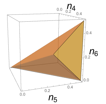
Figure 1: Polytope defined by the expression $n_{4}\leq n_{5}+n_{6}$, subject to the condition $0\leq n_{6}\leq n_{5}\leq n_{4}\leq 0.5$. The saturation condition $n_{5}+n_{6}=n_{4}$ is satisfied by the points on one of the faces of the polytope, whereas on the edges $n_{5}+n_{6}=0.5$ we have $n_{4}=0.5$ and for $n_{4}=n_{5}$ we have $n_{6}=0$. The single determinant state is placed at the lower left corner $n_{i}=0$ of the polytope.

The wave function for this configuration for $\wedge^{3}\mathcal{H}_{6}$ in the basis of natural orbitals can now be written in terms of the 1-RDM matrix:

$$|\Psi\rangle_{3,6} =c_{123}|\alpha_{1}\alpha_{2}\alpha_{3}\rangle+c_{145}|\alpha_{1}\alpha_{4}\alpha_{5}\rangle$$

$$\quad+c_{246}|\alpha_{2}\alpha_{4}\alpha_{6}\rangle;$$ (5)

with the proviso $|c_{123}|\geq|c_{145}|\geq|c_{246}|$. It is now patent that $|\Psi\rangle$ can be elegantly rewritten as

$$\sqrt{n_{3}}\,|\alpha_{1}\alpha_{2}\alpha_{3}\rangle+\sqrt{n_{5}}\,|\alpha_{1}\alpha_{4}\alpha_{5}\rangle+\sqrt{n_{6}}\,|\alpha_{2}\alpha_{4}\alpha_{6}\rangle,$$ (6)

in analogy to the Löwdin–Shull (LS) functional for the two-electron case LS . Note that, just like in the LS functional, only doubly excited configurations are here permitted Ccomment . (We understand excitations with respect to the “best density” Slater determinant, in the sense of KS68 .)

The pinned configuration

$$(n_{1},n_{2},n_{3})=\bigl{(}\tfrac{3}{4},\tfrac{3}{4},\tfrac{1}{2}\bigr{)}$$

is far from the “Hartree-Fock” $(1,1,1)$ state. Now, a little surprise awaits us: for spin-compensated, very strongly correlated systems it is possible to show by the same method as above, the following identity

$$n_{1}+n_{2}+n_{3} =2,$$

$$\quad\mbox{equivalently}\quad n_{4}+n_{5}+n_{6} =1.$$ (7)

In terms of $\rho_{1}$ the wave function then reads

$$|\Psi\rangle=\sqrt{n_{4}}|\alpha_{1}\alpha_{2}\alpha_{4}\rangle+\sqrt{n_{5}}|\alpha_{1}\alpha_{3}\alpha_{5}\rangle+\sqrt{n_{6}}|\alpha_{2}\alpha_{3}\alpha_{6}\rangle,$$

living in the $0$-eigenspace of the operator

$$\mathbf{2}-a^{\dagger}_{1}a_{1}-a^{\dagger}_{2}a_{2}-a^{\dagger}_{3}a_{3}.$$

We note that overlap of those wave functions with the $|\alpha_{1}\alpha_{2}\alpha_{3}\rangle$ state is zero. For the case $n_{4}=n_{5}=n_{6}=1/3$ this was already noted by Kutzelnigg and Smith KS68 . The Borland–Dennis–Klyachko constraint becomes in this case:

$$2-(n_{1}+n_{2}+n_{4})=n_{3}-n_{4}\geq 0.$$

Therefore in this regime it is possible to determine $|\Psi\rangle$ from $\rho_{1}$ even without Klyachko pinning. The border between the two regimes is given by the degeneracy line $n_{3}=n_{4}=\tfrac{1}{2}$. Inequality (4) together with the pinning (7) cut out a new facet on the polytope of allowed states (Fig. 2).

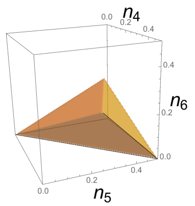
Figure 2: Polytope defined by the expression $n_{4}\leq n_{5}+n_{6}$, subject to the condition $0\leq n_{6}\leq n_{5}\leq n_{4}\leq 0.5$, plus the condition $n_{4}+n_{5}+n_{6}\leq 1$. The saturation condition $n_{4}+n_{5}+n_{6}=1$ is satisfied by the points on the face of the polytope whose vertices are $\bigl{(}\tfrac{1}{2},\tfrac{1}{2},0\bigr{)}$, $\bigl{(}\tfrac{1}{2},\tfrac{1}{4},\tfrac{1}{4}\bigr{)}$ and $\bigl{(}\tfrac{1}{3},\tfrac{1}{3},\tfrac{1}{3}\bigr{)}$.

In summary, the Borland–Dennis–Klyachko polytope of states is still too large. In fact, the spin-compensated states lie either on the $n_{1}+n_{2}+n_{4}=2$ facet of the polytope (when closer to the single-determinant state) or on the plane $n_{4}+n_{5}+n_{6}=1$ (when farther from the single-determinant state). The edge $n_{3}=n_{4}$ is shared by these two planes. Since the exact expressions given above for the spin-compensated formulation of the system $\wedge^{3}\mathcal{H}_{6}$ lead to a diagonal 1-RDM, without any restriction on the amplitudes $c_{ijk}$ (provided, of course, that the orbitals are orthonormal), for such a simple system one does not need a previous CI calculation to compute the natural orbitals and the value of the ground-state energy Oxford .

All of the 70 pure state Slater hull inequalities, grouped in four permutation classes, shown in DavidsonXX ; DavidsonXXI for expectation values of products of number operators can be derived trivially from the GPC by Klyachko; as an example:

$$\langle(a^{\dagger}_{a}a_{a}+a^{\dagger}_{b}a_{b})(a^{\dagger}_{c}a_{c}+a^{\dagger}_{d}a_{d})+a^{\dagger}_{a}a_{a}a^{\dagger}_{b}a_{b}$$

$$\quad+a^{\dagger}_{c}a_{c}a^{\dagger}_{d}a_{d}+a^{\dagger}_{e}a_{e}a^{\dagger}_{f}a_{f}\rangle\geq 1,\quad 1\leq a,b,c,d,e,f\leq 6.$$

Some are pinned. Lack of space prevents us from going into the details of this.

The converse statement looks unlikely to us.

IV Numerical investigations: lithium with broken spherical symmetry

In the previous paper Sybilla we obtained rank-six, -seven and -eight approximations for the lithium isoelectronic series by using a set of helium-like one-particle wave functions in addition to one hydrogen-like wave function. Guided by the classical work of Shull and Löwdin LS , for the former we employed the following set of orthonormal spatial orbitals:

$$\delta_{n}(\alpha,\bm{r}):=D_{n}\sqrt{\frac{\alpha^{3}}{\pi}}L^{2}_{n-1}\bigl{(}2\alpha r\bigr{)}e^{-\alpha r},\quad n=1,2,\ldots$$

where $D^{-2}_{n}=\binom{n-1}{2}$, and we use the standard definition of the associated Laguerre polynomials $L^{\zeta}_{n}$ reliablerussian . For the hydrogen-like function we used

$$\psi(\beta,\bm{r})=\frac{1}{4}\sqrt{\frac{\beta^{5}}{6\pi}}r\,e^{-\beta r/2}.$$

Applying a variational procedure for the state $|\delta_{1}{\mathord{\uparrow}}\delta_{1}{\mathord{\downarrow}}\psi{\mathord{\uparrow}}\rangle$ results in $\alpha=2.68$ and $\beta=1.27$, and the total energy associated to this Slater determinant becomes $-7.4179$ a.u., reasonably close to the Hartree–Fock energy $-7.4327$ a.u.

Now we examine the GPC when the spherical symmetry of the central potential is broken by considering the following Hamiltonian:

$$H(Z,\gamma)=\frac{1}{2}\sum^{3}_{i=1}|\bm{p}_{i}|^{2}$$ (8)

$$\quad-\sum^{3}_{i=1}\frac{Z}{|\bm{r}_{i}|}\bigg{(}1+\gamma\frac{x^{2}_{i}}{|\bm{r}_{i}|^{2}}\bigg{)}+\sum^{3}_{i\,<\,j}\frac{1}{|\bm{r}_{i}-\bm{r}_{j}|}.$$

The case $H(3,0)$ is the Hamiltonian of lithium, whose accurate energy value is $-7.47806$ a.u.

A motivation behind this model is to lift constraints on the possible occupation numbers due to the spherical symmetry of the isolated Li atom. Lowering the symmetry makes the model more flexible and allows to envisage more general cases. In addition, the model can serve to describe a Li atom embedded into some environment that does not provide covalent interactions with the Li atom. We have performed the calculations of this section by searching those values of $\alpha$ and $\beta$ for which the approximation to the ground state leads to the minimum energy with spin-compensated linear combinations of Slater determinants. Analytical expressions for the electron integrals were computed using Mathematica Mth and orthonormalized orbitals were obtained by the Gram–Schmidt procedure. Computations were performed with 36 decimals floating-point precision.

IV.1 Rank six

The spin-restricted rank-six approximation for $H(3,\gamma)$ is always pinned to the boundary of the polytope, as we already have shown in the general case in Section III. It is interesting to examine the spectral trajectory of the “best” spin-restricted state in $\wedge^{3}\mathcal{H}_{6}$ as a function of the parameter $\gamma$ by means of minimizing the CI states on the manifold $(\alpha,\beta)$. To this end we choose as a one-particle Hilbert space the set

$$\{\delta_{1}{\mathord{\uparrow}},\delta_{1}{\mathord{\downarrow}},\psi{\mathord{\uparrow}},\psi{\mathord{\downarrow}},\delta_{2}{\mathord{\uparrow}},\delta_{2}{\mathord{\downarrow}}\}.$$

The Hilbert space factorizes then in the direct product of two spin-orbital sectors $\wedge^{3}\,\mathcal{H}_{6}=\mathcal{H}_{3}\otimes\wedge^{2}\mathcal{H}_{3}$. There are nine configurations in all, eight of which belong to the $j=\tfrac{1}{2}$ representation,

$$|\delta_{1}{\mathord{\uparrow}}\delta_{1}{\mathord{\downarrow}}\psi{\mathord{\uparrow}}\rangle,\,|\delta_{1}{\mathord{\uparrow}}\delta_{1}{\mathord{\downarrow}}\delta_{2}{\mathord{\uparrow}}\rangle,\,|\psi{\mathord{\uparrow}}\psi{\mathord{\downarrow}}\delta_{1}{\mathord{\uparrow}}\rangle,\,|\psi{\mathord{\uparrow}}\psi{\mathord{\downarrow}}\delta_{2}{\mathord{\uparrow}}\rangle,$$

$$|\delta_{2}{\mathord{\uparrow}}\delta_{2}{\mathord{\downarrow}}\delta_{1}{\mathord{\uparrow}}\rangle,\,|\delta_{2}{\mathord{\uparrow}}\delta_{2}{\mathord{\downarrow}}\psi{\mathord{\uparrow}}\rangle,\,|\delta_{1}{\mathord{\uparrow}}\psi{\mathord{\downarrow}}\delta_{2}{\mathord{\uparrow}}\rangle-|\delta_{1}{\mathord{\downarrow}}\psi{\mathord{\uparrow}}\delta_{2}{\mathord{\uparrow}}\rangle,$$

$$|\delta_{1}{\mathord{\uparrow}}\psi{\mathord{\uparrow}}\delta_{2}{\mathord{\downarrow}}\rangle-|\delta_{1}{\mathord{\downarrow}}\psi{\mathord{\uparrow}}\delta_{2}{\mathord{\uparrow}}\rangle.$$

(The configuration $|\delta_{1}{\mathord{\uparrow}}\psi{\mathord{\downarrow}}\delta_{2}{\mathord{\uparrow}}\rangle+|\delta_{1}{\mathord{\downarrow}}\psi{\mathord{\uparrow}}\delta_{2}{\mathord{\uparrow}}\rangle+|\delta_{1}{\mathord{\uparrow}}\psi{\mathord{\uparrow}}\delta_{2}{\mathord{\downarrow}}\rangle$ belongs to the representation $j=\tfrac{3}{2}$.)

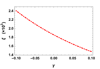
Figure 3: The distance $\xi$ between the spectrum of the ground state to the extreme point of the polytope as a function of $\gamma\in[-0.1,0.1]$ for the spin-restricted rank-six approximation to the Hamiltonian $H(3,\gamma)$ given by (8).

In order to quantify the position of the set of occupation numbers on the boundary of the polytope, one may define $\xi^{2}:=\sum_{i=1}^{3}(1-n_{i})^{2}$ as the euclidean distance between the spectrum of the state to the extreme point $(1,1,1)$ of the polytope, corresponding to the spectrum of a single determinant. Fig. 3 shows $\xi$ for small values of $\gamma$ of the electronic Hamiltonian given in (8). For decreasing $\gamma$ the spectrum of the one-body density departs further from that extremum. The kinematics however keeps the state pinned to the boundary of the Borland–Dennis–Klyahcko polytope, since its natural occupation numbers maintain the condition $1+n_{3}=n_{1}+n_{2}$.

A similar behavior is observed for a unrestricted description using, for instance, the set

$$\{\delta_{1}{\mathord{\uparrow}},\delta_{1}{\mathord{\downarrow}},\psi{\mathord{\uparrow}},\delta_{2}{\mathord{\uparrow}},\delta_{2}{\mathord{\downarrow}},\delta_{3}{\mathord{\uparrow}}\}$$

as the one-particle Hilbert space. However, the energy predicted by this latter configuration is slightly worse than the one predicted by the spin-restricted case.

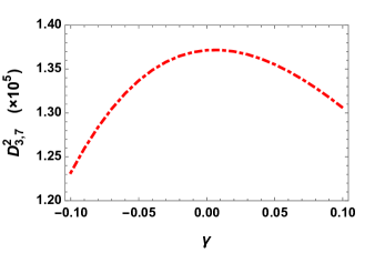
Figure 4: Second GPC $D^{2}_{3,7}$ for the ground-state of the Hamiltonian $H(3,\gamma)$ in a rank-seven approximation as a function of $\gamma\in[-0.1,0.1]$. For $\gamma=0.01$, the constraint reaches its maximum value (namely, $1.3717\times 10^{-5}$).

IV.2 Rank seven

There are four GPC for the three-electron system in a rank-seven configuration $\wedge^{3}\mathcal{H}_{7}$,

$$D^{1}_{3,7} =2-n_{1}-n_{2}-n_{4}-n_{7}\geq 0,$$

$$D^{2}_{3,7} =2-n_{1}-n_{2}-n_{5}-n_{6}\geq 0,$$

$$D^{3}_{3,7} =2-n_{2}-n_{3}-n_{4}-n_{5}\geq 0,$$

$$D^{4}_{3,7} =2-n_{1}-n_{3}-n_{4}-n_{6}\geq 0.$$ (9)

For lithium-like atoms, calculations Sybilla ; Mazziotti had shown that the first of these four inequalities is completely saturated.

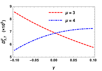
Figure 5: Third and fourth GPC for the ground-state of the Hamiltonian $H(3,\gamma)$ in a rank-seven approximation as a function of $\gamma\in[-0.1,0.1]$.

For the rank-seven approximation to the Hamiltonian (8), we choose

$$\{\delta_{1}{\mathord{\uparrow}},\delta_{1}{\mathord{\downarrow}},\psi{\mathord{\uparrow}},\delta_{2}{\mathord{\uparrow}},\delta_{2}{\mathord{\downarrow}},\delta_{3}{\mathord{\uparrow}},\delta_{3}{\mathord{\downarrow}}\}$$

as the one-particle Hilbert space. Other types of configurations are possible, too, but they lead to higher values for the ground-state energy. There are 18 configurations in total, but only 14 of them belong in the $j=\tfrac{1}{2}$ representation. For any $\gamma$, the occupation numbers satisfy

$$n_{1}+n_{2}+n_{4}+n_{7}=2\quad\mbox{and}\quad n_{3}+n_{5}+n_{6}=1,$$ (10)

implying that the first GPC of (9) is completely saturated. The Hilbert space of this system then splits into the direct product of two spin-orbital sectors $\wedge^{3}\,\mathcal{H}_{7}=\mathcal{H}_{3}\otimes\wedge^{2}\mathcal{H}_{4}$.

Also the following interesting system had been analyzed in Klyachko2 . The first excited state of beryllium, with spin $(\textbf{S},\mathbf{S}_{z})=(1,1)$, fills the lowest three shells $1s$, $2s$ and $2p$. In a reasonable approximation, the first natural orbital is completely occupied and the last two ones are empty (thus $n_{9}=n_{10}=0$). The seven remaining natural orbitals are organized in such a way that the first inequality in (9) is saturated, too.

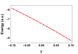
Figure 6: The ground-state energy for the spin-restricted rank-six approximation to the Hamiltonian $H(3,\gamma)$ given by (8) as a function of $\gamma\in[-0.1,0.1]$.

For lithium we found previously Sybilla that the GPC could be split into two groups differing in how close the equalities were obeyed, i.e., one may talk about two scales of quasipinning. Here we observe the same phenomenon. In fact, the value of the constraint $D^{2}_{3,7}$ is always below $1.3717\times 10^{-5}$, taking its maximum for $\gamma=0.01$ (i.e., practically at the “physical point”), as indicated in Fig. 4.

On the other hand, the remaining two GPC $D^{3}_{3,7}$ and $D^{4}_{3,7}$ take values around $7\times 10^{-5}$. As shown in Fig. 5, $D^{3}_{3,7}$ decreases when the value of $\gamma$ grows, while the last one increases when $\gamma$ increases. Notice the crossover of two constraints also close by $\gamma=0$.

IV.3 On the energies

Finally, Fig. 6 depicts the ground-state energy predicted by our model for the spin-restricted version of the rank-six approximation as a function of $\gamma$. For $H(3,0)$ the ground-state energy is $-7.4311$ a.u. For rank seven and $\gamma=0$, the calculated energy for this model is equal to $-7.4458$ a.u., lower than the Hartree–Fock energy for lithium. Remarkably, the rank-eight approximation for this model gives for the ground-state energy of lithium $-7.4548$ a.u., which represents more than $50\%$ of its correlation energy Sybilla .

V The molecular system $\mathrm{He}^{+}_{2}$

Rank	Energy	$n_{1}$	$n_{2}$	$n_{3}$	$n_{4}(10^{-3})$	$n_{5}(10^{-3})$	$n_{6}(10^{-3})$	$n_{7}(10^{-3})$	$n_{8}(10^{-4})$
6	$-4.9125$	0.9992	0.9949	0.9941	5.8086	5.0914	0.7172	-	-
7	$-4.9194$	0.9973	0.9941	0.9915	7.1019	5.8950	2.5530	1.3220	-
8	$-4.9239$	0.9968	0.9932	0.9901	8.4888	6.8304	3.0819	1.3665	0.1178

Table 1: Occupation numbers and energies for rank-six to rank-eight for He${}_{2}^{+}$ in its equilibrium geometry, employing 6-31G basis set.

In this section we study the behavior of the occupation numbers of helium’s molecular ion He${}^{+}_{2}$. The goal is to explore the GPC along the dissociation path of this three-electron system, whose symmetry is lower than spherical, identifying those almost saturated. The Hartree-Fock energy for this system is $-4.9$ a.u. data , with a 6-31G basis set. The equilibrium bond length is $2.08$ a.u. data . The computed value for the ground-state energy is approximately $-4.99$ a.u. exphe ; data . Therefore the correlation energy is equal to $90$ mHa. We have approximated the atomic orbitals by employing a 6-31G basis set STO . We here report our results for (rank six, seven and eight) CI approximations for this diatomic ion.

V.1 GPC for the He${}^{+}_{2}$ ground state

For a dimer with atomic charges $Z$ the energy is given by the expression

$$-\int\bigg{(}\frac{1}{2}\nabla^{2}_{\bm{r}}+\sum_{\mu\in\{A,B\}}\frac{Z}{|\bm{r}-\bm{R}_{\mu}|}\bigg{)}\,\rho_{1}(\bm{x},\bm{x}^{\prime})\bigg{|}_{\bm{x}=\bm{x}^{\prime}}\,d\bm{x}$$

$$\qquad+\int\frac{\rho_{2}(\bm{x}_{1},\bm{x}_{2})}{|\bm{r}_{1}-\bm{r}_{2}|}\,d\bm{x}_{1}\,d\bm{x}_{2}+\frac{Z^{2}}{|\bm{R}|}$$

The two atoms are located at $\bm{R}_{A}$ and $\bm{R}_{B}$ and separated by $\bm{R}:=\bm{R}_{A}-\bm{R}_{B}$. The standard quantum-chemical notation $\bm{x}:=(\bm{r},\varsigma)$, with $\varsigma\in\{{\mathord{\uparrow}},{\mathord{\downarrow}}\}$ is employed. The molecular orbitals are constructed as linear combinations of the atomic $1s$ and $2s$ orbitals, which are in turn solutions of the Hartree-Fock equations. In the rest of this subsection, standard notation for the bonding (gerade) and antibonding (ungerade) molecular orbitals is used. The ground-state configuration of He${}^{+}_{2}$ is classified as ${}^{2}\Sigma_{u}$ and the starting configuration is a single Slater determinant, $|1\sigma_{g}^{{\mathord{\uparrow}}}1\sigma_{g}^{{\mathord{\downarrow}}}1\sigma^{{\mathord{\uparrow}}}_{u}\rangle$.

Table 1 presents the results for the energy and for the natural orbital occupancy numbers from rank-six up to rank-eight approximations for the ground-state of He${}_{2}^{+}$. The rank-six approximation is obtained through a spin-compensated configuration,

$$\{1\sigma_{g}^{\mathord{\uparrow}},1\sigma_{g}^{\mathord{\downarrow}},1\sigma_{u}^{\mathord{\uparrow}},1\sigma_{u}^{\mathord{\downarrow}},2\sigma_{g}^{\mathord{\uparrow}},2\sigma_{g}^{\mathord{\downarrow}}\}.$$

Higher-rank configurations are obtained by successively adding the orbitals $\{2\sigma_{u}^{\mathord{\uparrow}},2\sigma_{u}^{\mathord{\downarrow}}\}$.

Generalized Pauli conditions for $\wedge^{3}\mathcal{H}_{8}$	$\times 10^{3}$
$0\leq\mathcal{D}^{1}_{3,8}=2-(n_{1}+n_{2}+n_{4}+n_{7})$	0.0570
$0\leq\mathcal{D}^{2}_{3,8}=2-(n_{1}+n_{2}+n_{5}+n_{6})$	0
$0\leq\mathcal{D}^{3}_{3,8}=2-(n_{2}+n_{3}+n_{4}+n_{5})$	1.2712
$0\leq\mathcal{D}^{4}_{3,8}=2-(n_{1}+n_{3}+n_{4}+n_{6})$	1.4854
$0\leq\mathcal{D}^{5}_{3,8}=1-(n_{1}+n_{2}-n_{3})$	0.0452
$0\leq\mathcal{D}^{6}_{3,8}=1-(n_{2}+n_{5}-n_{7})$	1.2594
$0\leq\mathcal{D}^{7}_{3,8}=1-(n_{1}+n_{6}-n_{7})$	1.4736
$0\leq\mathcal{D}^{8}_{3,8}=1-(n_{2}+n_{4}-n_{6})$	1.3164
$0\leq\mathcal{D}^{9}_{3,8}=1-(n_{1}+n_{4}-n_{5})$	1.5306
$0\leq\mathcal{D}^{10}_{3,8}=1-(n_{3}+n_{4}-n_{7})$	2.7449
$0\leq\mathcal{D}^{11}_{3,8}=1-(n_{1}+n_{8})$	3.1772
$0\leq\mathcal{D}^{12}_{3,8}=-(n_{2}-n_{3}-n_{6}-n_{7})$	1.3046
$0\leq\mathcal{D}^{13}_{3,8}=-(n_{4}-n_{5}-n_{6}-n_{7})$	2.7901
$0\leq\mathcal{D}^{14}_{3,8}=-(n_{1}-n_{3}-n_{5}-n_{7})$	1.5188
$0\leq\mathcal{D}^{15}_{3,8}=2-(n_{2}+n_{3}+2n_{4}-n_{5}-n_{7}+n_{8})$	7.7980
$0\leq\mathcal{D}^{16}_{3,8}=2-(n_{1}+n_{3}+2n_{4}-n_{5}-n_{6}+n_{8})$	5.9792
$0\leq\mathcal{D}^{17}_{3,8}=2-(n_{1}+2n_{2}-n_{3}+n_{4}-n_{5}+n_{8})$	5.0983
$0\leq\mathcal{D}^{18}_{3,8}=2-(n_{1}+2n_{2}-n_{3}+n_{5}-n_{6}+n_{8})$	3.0082
$0\leq\mathcal{D}^{19}_{3,8}=-(n_{1}+n_{2}-2n_{3}-n_{4}-n_{5})$	5.4973

Table 2: First 19 GPC for the system $\wedge^{3}\mathcal{H}_{8}$ and numerical values for $\mathrm{He}^{+}_{2}$ at its equilibrium geometry.

A number of findings can now be identified.

• For rank six, the spin-compensated configuration gives the Borland–Dennis–Klyachko saturation condition $1+n_{3}=n_{1}+n_{2}$.

• For rank seven, we obtain the following values for the GPC:

  $$D^{1}_{3,7} =2.42\times 10^{-5},\;D^{2}_{3,7}=0,$$

  $$D^{3}_{3,7} =1.24\times 10^{-3},\;D^{4}_{3,7}=1.39\times 10^{-3}.$$

  The constraint due to spin has “jumped”, with respect to the lithium series!

• For this latter rank, two scales of quasipinning are clearly identified. Compared with the lithium-like atom, the first level of quasipinning is here more meaningful and probably more useful in order to reduce the number of Slater determinants, since the distance to the “Hartee-Fock” point is here bigger, namely, $\xi=1.06\times 10^{-2}$.

It is a fact of life that the number of GPC grows very rapidly with rank. For rank eight there are 31 inequalities Alturulato . They have been listed in a plain-text format Data . Of those, 19 constraints are given in Table 2. The first four are equal to the Klyachko conditions for $\wedge^{3}\mathcal{H}_{7}$.

Several scales of quasipinning can be identified here, as well. Most important is the robustness of quasipinning. In particular, the quantity $D^{2}_{3,8}$, found to be exactly zero in the previous rank, remains in a saturated regime. The first and fifth inequality belong to a strongly quasi-pinned regime, too. For the remaining inequalities we have

$$D^{2}_{3,8}\leq D^{5}_{3,8}\leq D^{1}_{3,8}\leq D^{6}_{3,8}\leq D^{3}_{3,8}$$

$$\leq D^{12}_{3,8}\leq D^{8}_{3,8}\leq D^{7}_{3,8}\leq D^{4}_{3,8}\leq\cdots.$$

V.2 Occupation numbers and potential curves

Potential energy curves for the three different ranks of the CI approximation for He${}^{+}_{2}$ are presented in Fig. 7. At the equilibrium geometry, as also seen in Table 1, a larger rank results in a lower ground-state energy. All approximations behave similarly around the equilibrium distance. At large interatomic distances, the value predicted by the rank-eight configuration is $-4.845$ a.u. which is to be compared with the total energy of the two separated compounds (He and He⁺): $-4.903$ a.u. inonization .

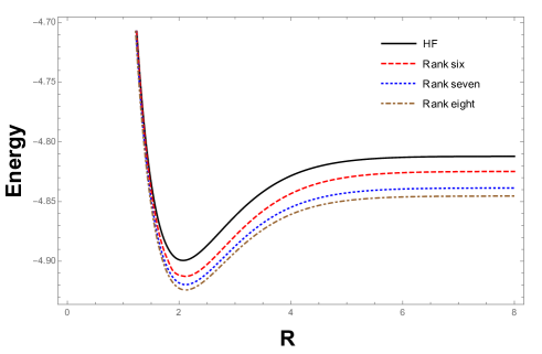
Figure 7: He${}^{+}_{2}$ potential energy curves for the three ranks of CI approximation $\wedge^{3}\mathcal{H}_{m}$, $m\in\{3,6,7,8\}$ using 6-31G as a basis set.

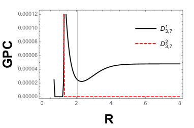
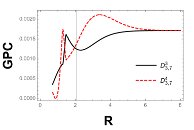
Figure 8: Rank-seven GPC as functions of the interatomic distance in atomic units. The vertical lines mark the equilibrium bond length.

Fig. 8 displays rank-seven GPC as functions of the interatomic distance in atomic units. There are again two scales of quasipinning. The first two GPC remain in a strongly pinned regime, since for those $D_{3,7}^{\mu}$ is very close to 0. For those, we notice a sharp crossover at lengths shorter than that of equilibrium. In fact, one of them is always completely saturated: in the region $R<1.25$ a.u., i.e., $D^{1}_{3,7}=0$ is a very good approximation, whereas for $R>1.25$ a.u. $D^{2}_{3,7}=0$ is also very good. Unfortunately, we do not have yet a good description for this apparent quenching of degrees of freedom, which surely deserves further investigation.

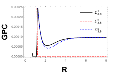
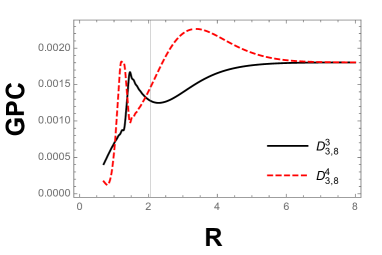
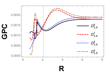
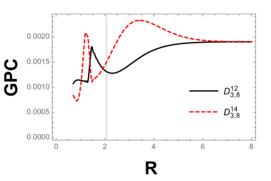
Figure 9: Rank-eight GPC as functions of the interatomic distance. The vertical lines mark the equilibrium bond length.

For rank eight, several scales of quasipinning can be observed for He${}^{+}_{2}$. Our main result is again the robustness of quasipinning. In particular, we observe that the quantities $D^{1}_{3,8}$ and $D^{2}_{3,8}$, found to be exactly zero for some bond-length regime at rank seven, remain in a strongly saturated regime, as shown in Fig. 9. The Hilbert space of this system splits then into the direct product of two spin-orbital sectors $\wedge^{3}\,\mathcal{H}_{8}=\mathcal{H}_{4}\otimes\wedge^{2}\mathcal{H}_{4}$. Also $D^{5}_{3,8}$ is found to be very close to 0.

To a second quasipinning regime belong the quantities

$$D^{3}_{3,8},D^{4}_{3,8},D^{6}_{3,8},D^{7}_{3,8},D^{8}_{3,8},D^{9}_{3,8},D^{12}_{3,8},D^{14}_{3,8}.$$

As seen in Fig. 9, these GPC behave roughly in the same way for increasing bond length. Their values tend asymptotically to approximately the same value for large interatomic distances.

Finally, a third quasipinning sector appears to be composed by $D^{10}_{3,8},D^{13}_{3,8},D^{15}_{3,8},D^{18}_{3,8},D^{19}_{3,8}$.

VI Quasipinning and excitations

From the seminal work by Löwdin and Shull it is known that the transformation to natural orbitals removes all single (S) excitations of the wave function of two-electron systems LS . For the singlet state the general wave function can be written exactly as

$$|\Psi(\bm{x}_{1},\bm{x}_{2})\rangle=\frac{1}{\sqrt{2}}({\mathord{\uparrow}}_{1}{\mathord{\downarrow}}_{2}-{\mathord{\downarrow}}_{1}{\mathord{\uparrow}}_{2})\sum^{\infty}_{i=1}c_{i}|\alpha_{i}(\bm{r}_{1})\alpha_{i}(\bm{r}_{2})\rangle.$$

Again, we have used $\bm{x}:=(\bm{r},\varsigma)$ with $\varsigma$ being the spin coordinates $\{{\mathord{\uparrow}},{\mathord{\downarrow}}\}$. A similar expression can be found for the triplet state Laetitia .

It is also remarkable that the wave function (5) does not contain S or triple (T) excitations of the best single-determinant state $|0\rangle:=|\alpha_{1}\alpha_{2}\alpha_{3}\rangle$. The Slater determinants $|\alpha_{1}\alpha_{4}\alpha_{5}\rangle$ and $|\alpha_{2}\alpha_{4}\alpha_{6}\rangle$ correspond to double (D) excitations of this state.

Single excitations cannot be completely removed from the CI wave function of general many-electron systems when written in terms of natural orbitals. However, Mentel and coworkers Grillo have recently shown that writing the wave function in the basis of natural orbitals leads to a sharp drop of the coefficients of Slater determinants containing just S excitations. For the BH molecule, the sum of squares of CI coefficients of singles falls from $1.5\times 10^{-3}$ to $5.3\times 10^{-6}$ when switching to the natural orbital basis. In this section and the next we argue that this phenomenon is a consequence from the near-saturation of some Klyachko selection rules on the occupation numbers.

VI.1 Selection rule for excitations in $\wedge^{3}\mathcal{H}_{6}$

This case has been just discussed. Even if the number of basis spin orbitals pointing up is different of the number of the ones pointing down, an eventual saturation of condition (4) would lead to the situation summarized in Table 3. A double excitation is also removed thereby.

Condition	$|0\rangle$	S	D	T	Total
CI	1	3	3	1	8
$\mathbf{D}^{1}_{3,6}|\Psi\rangle=0$	1	0	2	0	3

Table 3: Number of Slater determinants in the total and force-pinned CI expansions of the wave function for the system $\wedge^{3}\mathcal{H}_{6}$.

VI.2 Selection rules for excitations in $\wedge^{3}\mathcal{H}_{7}$

The four Klyachko inequalities for the three-electron system in a rank-seven approximation $\wedge^{3}\mathcal{H}_{7}$ were given in Eq. (9). The corresponding operators are

$$\mathbf{D}^{1}_{3,7} =2-a^{\dagger}_{1}a_{1}-a^{\dagger}_{2}a_{2}-a^{\dagger}_{4}a_{4}-a^{\dagger}_{7}a_{7},$$

$$\mathbf{D}^{2}_{3,7} =2-a^{\dagger}_{1}a_{1}-a^{\dagger}_{2}a_{2}-a^{\dagger}_{5}a_{5}-a^{\dagger}_{6}a_{6},$$

$$\mathbf{D}^{3}_{3,7} =2-a^{\dagger}_{2}a_{2}-a^{\dagger}_{3}a_{3}-a^{\dagger}_{4}a_{4}-a^{\dagger}_{5}a_{5},$$

$$\mathbf{D}^{4}_{3,7} =2-a^{\dagger}_{1}a_{1}-a^{\dagger}_{3}a_{3}-a^{\dagger}_{4}a_{4}-a^{\dagger}_{6}a_{6}.$$

As discussed above, for the lithium isoelectronic series Sybilla , for the system described by the Hamiltonian of Eq. (8) and for the first excited state of beryllium in a rank-ten approximation Klyachko2 , the first of the four inequalities (9) is completely saturated. Accordingly, for all these systems, the exact wave function satisfies the condition

$$\mathbf{D}^{1}_{3,7}|\Psi\rangle_{3,7}=0.$$

This implies that in the natural orbital basis, every Slater determinant is composed of three natural orbitals, two of them belonging to the set $\{\alpha_{1},\alpha_{2},\alpha_{4},\alpha_{7}\}$ and one belonging to the set $\{\alpha_{3},\alpha_{5},\alpha_{6}\}$. Then, the system $\wedge^{3}\mathcal{H}_{7}$ is reduced to $\mathcal{H}_{3}\otimes\wedge^{2}\mathcal{H}_{4}$, with in total eighteen of those Slater determinants.

Imposing as well saturation of the second inequality of (9), i.e., $\mathbf{D}^{2}_{3,7}\mathbf{D}^{1}_{3,7}|\tilde{\Psi}\rangle_{3,7}=0$, the singles and the triples are completely removed from the expression, as shown in Table 4. The corresponding wave function $|\tilde{\Psi}\rangle_{3,7}$ is written in terms of the inicial configuration $|\alpha_{1}\alpha_{2}\alpha_{3}\rangle$, plus the following eight D configurations:

$$|\alpha_{1}\alpha_{4}\alpha_{5}\rangle,|\alpha_{2}\alpha_{4}\alpha_{6}\rangle,|\alpha_{1}\alpha_{5}\alpha_{7}\rangle,|\alpha_{2}\alpha_{5}\alpha_{7}\rangle,$$

$$|\alpha_{1}\alpha_{4}\alpha_{6}\rangle,|\alpha_{2}\alpha_{4}\alpha_{5}\rangle,|\alpha_{1}\alpha_{6}\alpha_{7}\rangle,|\alpha_{2}\alpha_{6}\alpha_{7}\rangle.$$ (11)

Condition	$|0\rangle$	S	D	T	Total
$\mathbf{D}^{1}_{3,7}|\Psi\rangle_{3,7}=0$	1	6	9	2	18
$\mathbf{D}^{2}_{3,7}\mathbf{D}^{1}_{3,7}|\tilde{\Psi}\rangle_{3,7}=0$	1	0	8	0	9

Table 4: Number of Slater determinants in the total and force-pinned CI expansions of the wave function for the system $\wedge^{3}\mathcal{H}_{7}$.

VI.3 Selection rules for excitations in $\wedge^{3}\mathcal{H}_{8}$

The empirical evidence discussed earlier shows that the inequalities for the following GPC are almost or completely saturated:

$$D^{1}_{3,8},D^{2}_{3,8},D^{5}_{3,8}.$$

Imposing the saturation of the second and fifth constraints, say, the singles and the triples are removed completely, as shown in Table 5. The corresponding wave function $|\tilde{\Psi}\rangle_{3,8}$ is written in terms of the 9 configurations of the pinned rank-seven wave function (11), plus the configurations

$$|\alpha_{1}\alpha_{5}\alpha_{8}\rangle,|\alpha_{2}\alpha_{6}\alpha_{8}\rangle,|\alpha_{2}\alpha_{5}\alpha_{8}\rangle,|\alpha_{1}\alpha_{6}\alpha_{8}\rangle.$$

Condition	$|0\rangle$	S	D	T	Total
$\mathbf{D}^{2}_{3,8}|\Psi\rangle_{3,8}=0$	1	7	13	3	24
$\mathbf{D}^{5}_{3,8}\mathbf{D}^{2}_{3,8}|\tilde{\Psi}\rangle_{3,8}=0$	1	0	12	0	13

Table 5: Number of Slater determinants in the total and force-pinned CI expansions of the wave function for the system $\wedge^{3}\mathcal{H}_{8}$.

VI.4 He${}^{+}_{2}$: electronic energy and pinning truncations

An idea behind quasipinning is to approximate the wave function through a truncated expansion by using the selection rules that emerge after imposing pinning. Therefore, it is a relevant issue to examine how the electronic energy is affected as the number of configurations is reduced in the truncation. Here we explore the ground-state energy for the helium dimer He${}^{+}_{2}$ for different pinned wave functions, compared with the energy predicted by the CI expansion within the same rank. (It must be said beforehand that, contrarily to the case of lithium-like systems, up to rank eight less than 30% of the absolute correlation energy is recovered. This is due partly to a less than optimal choice of the basis set, partly to the the difficulty to capture some aspects of correlation with such short basis sets.)

Table 6 contains the value of the correlation energy for (force-pinned and complete) wave functions for the rank-six up to -eight approximations for the ground state of He${}^{+}_{2}$.

It is remarkable that the force-pinned wave function $|\tilde{\Psi}\rangle_{3,7}$ reconstructs $99.79$%  of the rank-seven correlation energy, employing just 9 configurations. The CI rank-eight wave function contains 24 Slater determinants belonging to the Hilbert space $\wedge^{2}\mathcal{H}_{4}\otimes\mathcal{H}_{4}$. The correlation energy is 24.64 mHa. The pinned wave function $|\tilde{\Psi}\rangle_{3,8}$ reconstructs $99.51$%  of this available correlation energy, employing 13 Slater determinants.

Wave function	$|E-E_{\mathrm{HF}}|$
$|\Psi\rangle_{3,6}$	13.22
$|\tilde{\Psi}\rangle_{3,6}$	13.22
$|\tilde{\Psi}\rangle_{3,7}$	20.12
$|\Psi\rangle_{3,7}$	20.17
$|\tilde{\Psi}\rangle_{3,8}$	24.56
$|\Psi\rangle_{3,8}$	24.64

Table 6: Ground-state correlation energies predicted for the complete and force-pinned CI wave functions for He${}^{+}_{2}$ in the rank-six up to rank-eight approximations. The values are given in mHa.

Fig. 10 shows the absolute value of the correlation energy along the dissociation path for CI rank-six up to rank-eight expansions ($|\Psi\rangle_{3,6}$, $|\Psi\rangle_{3,7}$, $|\Psi\rangle_{3,8}$) and for the pinned wave functions $|\tilde{\Psi}\rangle_{3,7}$ and $|\tilde{\Psi}\rangle_{3,8}$. It is also remarkable that the pinned rank-seven and rank-eight wave functions almost contain the complete correlation energy to the corresponding rank of approximation along the complete path, demonstrating the negligible role of the single and triple excitations. These results suggest that in spite that saturation of one GPC reduces notably the number of Slater determinants, remarkably good values for the correlation energies are obtained.

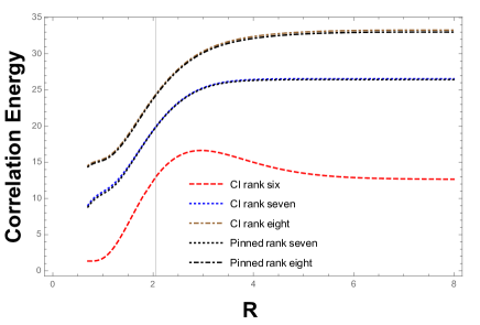
Figure 10: Absolute value of the correlation energy $|E-E_{HF}|$ for CI expansion and pinned wave functions for ranks-six up to rank-eight approximations, along the dissociation path for He${}^{+}_{2}$. Pinned wave function $|\tilde{\Psi}\rangle_{3,6}$ is equivalent to the CI rank-six expansion, so it is not included. The values are given in mHa.

VII On four-electron systems

For the case of a four-electron system with a 8-dimensional one-electron Hilbert space, $\wedge^{4}\mathcal{H}_{8}$, there are in total $14$ generalized Pauli conditions. Derived initially by Klyachko Alturulato , they read

$$D^{\mu}_{4,8} :=\sum^{8}_{i=1}\kappa^{\mu}_{i}n_{i}\geq 0,$$

$$D^{7+\mu}_{4,8} :=2-\sum^{8}_{i=1}\kappa^{\mu}_{9-i}n_{i}\geq 0,$$ (12)

for $1\leq\mu\leq 7$ and provided that $n_{1}\leq 1$. The coefficients $\kappa^{\mu}_{i}$ are given in Table 7.

$\mu$	$\kappa^{\mu}_{1}$	$\kappa^{\mu}_{2}$	$\kappa^{\mu}_{3}$	$\kappa^{\mu}_{4}$	$\kappa^{\mu}_{5}$	$\kappa^{\mu}_{6}$	$\kappa^{\mu}_{7}$	$\kappa^{\mu}_{8}$
1	$-1$	0	0	1	0	1	1	0
2	$-1$	0	0	1	1	0	0	1
3	$-1$	0	1	0	0	1	0	1
4	$-1$	1	0	0	0	0	1	1
5	0	$-1$	0	1	0	1	0	1
6	0	0	$-1$	1	0	0	1	1
7	0	0	0	0	$-1$	1	1	1

Table 7: Sets of coefficients for the generalized Pauli conditions of (12) for the system $\wedge^{4}\mathcal{H}_{8}$.

For quantum states with an even number of fermions, vanishing total spin and time-reversal symmetry, Smith proved that a 1-RDM is pure $N$-representable if and only if all its eigenvalues are doubly degenerated Smith . Therefore, for these systems, the occupation numbers obey

$$n_{2i-1}=n_{2i}\qquad\qquad i=1,2,\cdots.$$ (13)

The double degeneracy of the occupation numbers forces the generalized Pauli conditions for the system $\wedge^{4}\mathcal{H}_{8}$ to reduce to the traditional Pauli exclusion principle Mazziotti . Therefore, a state will be pinned only if it is pinned to the traditional Pauli conditions, which only occurs for a single-determinant wave function. For instance,

$$D^{1}_{4,8} :=-n_{1}+n_{4}+n_{6}+n_{7}=2(1-n_{1}),$$

$$D^{8}_{4,8} :=2-n_{2}-n_{3}-n_{5}+n_{8}=2n_{8},$$

$$D^{14}_{4,8} :=2-n_{1}-n_{2}-n_{3}+n_{4}=2(1-n_{1}).$$

Chakraborty and Mazziotti Mazziotti  computed the occupation numbers for the ground state of some four-electron molecules for rank equal to twice the number of electrons, employing a STO-3G basis set. In this range of approximation, the two energetically lowest orbitals of LiH are completely occupied (therefore $D^{1}_{4,8}=0$) and the Shull–Löwdin functional guarantees that doubly excited determinants completely govern rank-eight CI calculations for this molecule.

However, there are important effects of dynamical electron correlation which involve the core electrons and the molecule cannot be considered as a two-electron system. In fact, for higher ranks the two biggest occupation numbers ($n_{1}=n_{2}$) become smaller than 1. The first (and the second as well) occupation number of BH is very close to 1 and accordingly $D^{1}_{4,8}$ is quasipinned. For LiH and BeH₂, the seventh occupation number is almost 0 and hence for these systems $D^{8}_{4,8}$ is quasipinned.

In a spin-compensated description, the system $\wedge^{4}\mathcal{H}_{8}$ with total spin component $\mathbf{S}_{z}$ equal to 1 contains 16 configurations, corresponding to $\wedge^{3}\mathcal{H}_{4}\otimes\mathcal{H}_{4}$. The CI expansion only contains double or single excitations. In a spin-uncompensated description, the system $\wedge^{4}\mathcal{H}_{8}$ with total spin component $\mathbf{S}_{z}$ equal to one would contain 30 configurations, corresponding to $\wedge^{3}\mathcal{H}_{5}\otimes\mathcal{H}_{3}$. Notice that if the GPC

$$D^{14}_{4,8}=2-n_{1}-n_{2}-n_{3}+n_{4}\geq 0$$ (14)

were completely saturated, the corresponding wave function is a member of the 0-eigenspace of the operator:

$$\mathbf{D}^{14}_{4,8} =2-a^{\dagger}_{1}a_{1}-a^{\dagger}_{2}a_{2}-a^{\dagger}_{3}a_{3}+a^{\dagger}_{4}a_{4}.$$ (15)

and, for both configurations, single and triple excitations are entirely suppressed. This is a non-trivial fact. See Tables 8 and . Besides the initial configuration $|\alpha_{1}\alpha_{2}\alpha_{3}\alpha_{4}\rangle$, the configurations present in the expansion are just double excitations of this state which, in addition, do not contain the fourth natural orbital $\alpha_{4}$.

Condition	$|0\rangle$	S	D	T	Total
CI	1	6	9	0	16
$\mathbf{D}^{14}_{4,8}|\Psi\rangle=0$	1	0	9	0	10

Table 8: Number of Slater determinants in the full and pinned CI expansions of the wave function for the spin-restricted system $\wedge^{4}\mathcal{H}_{8}$ with $\mathbf{S}_{z}=1$.

In general, for the system $\wedge^{N}\mathcal{H}_{m}$, the condition

$$(N-2)+n_{N}=n_{1}+\cdots+n_{N-1}$$

has as consequence that only double excitations become the relevant configurations in a CI expansion Kassandra . Moreover, the only configuration containing the orbital $\alpha_{N}$ is $|\alpha_{1}\alpha_{2}\cdots\alpha_{N}\rangle$.

Condition	$|0\rangle$	S	D	T	Total
CI	1	8	16	5	30
$\mathbf{D}^{14}_{4,8}|\Psi\rangle=0$	1	0	11	0	12

Table 9: Number of Slater determinants in the full and pinned CI expansions of the wave function for the spin-unrestricted system $\wedge^{4}\mathcal{H}_{8}$ with $\mathbf{S}_{z}=1$.

For the larger system $\wedge^{4}\mathcal{H}_{10}$, the occupation numbers are bounded by 121 constraints Alturulato ; Data . We postpone their study.

VIII Conclusion

The recent solution of the pure $N$-representability problem, due to Klyachko, promises to generate a wide set of conditions (the GPC) on the natural occupation numbers for fermionic systems. The Klyachko algorithm does indeed produce sets of linear inequalities with integer coefficients for those numbers. The derivation of these inequalities, and of their consequences, is still a work in progress.

For reasons that nobody has been quite able to fathom yet, some of these inequalities appear to be nearly saturated, in a far from random way —this is the quasipinning phenomenon. A research program is born around these facts.

By means both of theoretical and numerical results, in this paper we have continued to explore the nature of pinning and quasipinning in some atomic and molecular models (mainly perturbed lithium with broken spherical symmetry and the dimer ion He${}^{+}_{2}$), for several finite rank approximations whose GPC are known.

We sum up our opinions on the outcomes of that program, so far.

• Saturation of some of the GPC leads to strong selection rules for identifying the most (in)effective configurations in CI expansions. In simple cases, this gives means for reducing the number of Slater determinants in the CI picture and therefore reducing computational requirements ETH ; Sybilla ; Klyachko2 . In general, it does provide insights in the structure of the wave function, which brute force methods are unable to.

• However, it is unlikely that Klyachko paradigm be relevant for computational quantum chemistry, at least in the short run. The main problem is the dramatic increase of the number of GPC with the rank of the spin orbital systems introduced in the calculations.

• The robustness of the almost saturation of a particular type of constraint conspires to “explain” why double excitations govern CI calculations of electron correlation, when using natural orbitals.

• A natural question is whether the exact “Löwdin–Shull” formula (6) for three-electron systems can be generalized to higher rank. The answer is a qualified, approximate yes, the price to pay being to invoke a second type of constraint less strongly quasi-pinned that the one referred to in the previous point. We refrain form going into the details here.

• A very promising avenue of research is to use the GPC to improve on the 1-RDM theory. There are now in the literature quite a few physically motivated density matrix functionals, built from the knowledge of the natural orbitals and occupation numbers, which can be traced back to the one proposed by Müller thirty years ago Muller ; they have mostly amounted to figure out Ansätze for reasonable two-body reduced density matrices, failing to date to fulfill a physical requirement or another Marmulla . The approach discussed in this paper suggests to construct 1-RDM by restricting the minimization set to the subset of GPC-honest systems. A promising start in this direction is Halle .

- (1) A. J. Coleman, Rev. Mod. Phys. 35, 668 (1963).
- (2) R. E. Borland and K. Dennis, J. Phys. B 5, 7 (1972).
- (3) A. Klyachko, J. Phys.: Conf. Ser. 36, 72 (2006).
- (4) M. Altunbulak and A. Klyachko, Commun. Math. Phys. 282, 287 (2008).
- (5) C. Schilling, D. Gross and M. Christandl, Phys. Rev. Lett. 110, 040404 (2013).
- (6) C. L. Benavides-Riveros, J. M. Gracia-Bondía, and M. Springborg, Phys. Rev. A 88, 022508 (2013).
- (7) R. Chakraborty and D. A. Mazziotti, Phys. Rev. A 89, 042505 (2014).
- (8) C. L. Benavides-Riveros and C. Schilling, in preparation.
- (9) I. Theophilou, N. N. Lathiotakis, M. A. L. Marques and N. Helbig, arXiv:1503.00746.
- (10) R. Chakraborty and D. A. Mazziotti, Phys. Rev. A 91, 010101(R) (2015).
- (11) J. Ivanic and K. Ruedenberg, Theor. Chem. Acc. 106, 339 (2001).
- (12) E. Giner, A. Scemama and M. Caffarel, Can. J. Chem. 91, 879 (2013).
- (13) A. Klyachko, arXiv:0904.2009.
- (14) C. Schilling, Phys. Rev. A 91, 022105 (2015).
- (15) W. B. McRae and E. R. Davidson, J. Math. Phys. 13, 1527 (1972).
- (16) E. R. Davidson, Comp. Theor. Chem. 1003, 28 (2013).
- (17) R. Pauncz, Spin Eigenfunctions: Construction and use, Plenum Press, New York, 1979.
- (18) M. Walter, Multipartite Quantum States and their Marginals, PhD thesis, ETH, Zürich (2014).
- (19) A. Lopes, D. Gross and C. Schilling, to appear.
- (20) P.-O. Löwdin and H. Shull, Phys. Rev. 101, 1730 (1956).
- (21) C. Schilling pointed to us at once that there is no ambiguity of signs in display (6).
- (22) W. Kutzelnigg and V. H. Smith, Int. J. Quant. Chem. 11, 531 (1968).
- (23) N. N. Lebedev, Special Functions and their Applications, Dover, New York, 1972.
- (24) Wolfram Research, Mathematica, Version 10.0, Champaign, IL (2014).
- (25) R. D. Johnson, Computational Chemistry Comparison and Benchmark Database, Tech. Rep. 101 Release 16a (NIST, 2013).
- (26) J. Xie, B. Poirier, and G. I. Gellene, J. Chem. Phys. 122, 184310 (2005).
- (27) W. J. Hehre, R. Ditchfield and J. A. Pople, J. Chem. Phys. 56, 2257 (1972).
- (28) Supplementary material in reference Alturulato .
- (29) A. E. Nilsson and S. Johansson, Phys. Scr. 44, 226 (1991).
- (30) C. L. Benavides-Riveros, J. M. Gracia-Bondía and J. C. Várilly, Phys. Rev. A 86, 022525 (2012).
- (31) Ł. M. Mentel, R. van Meer, O. V. Gritsenko, and E. J. Baerends, J. Chem. Phys. 140, 214105 (2014).
- (32) D. W. Smith, Phys. Rev. 147, 896 (1966).
- (33) C. L. Benavides-Riveros, J. M. Gracia-Bondía and M. Springborg, arXiv:1409.6435.
- (34) A. M. K. Müller, Phys. Lett. A 105, 446 (1984).
- (35) C. L. Benavides-Riveros and J. C. Várilly, Eur. Phys. J. D 22, 274 (2012).