Parallelized event chain algorithm for dense hard sphere and polymer systems

Abstract

We combine parallelization and cluster Monte Carlo for hard sphere systems and present a parallelized event chain algorithm for the hard disk system in two dimensions. For parallelization we use a spatial partitioning approach into simulation cells. We find that it is crucial for correctness to ensure detailed balance on the level of Monte Carlo sweeps by drawing the starting sphere of event chains within each simulation cell with replacement. We analyze the performance gains for the parallelized event chain and find a criterion for an optimal degree of parallelization. Because of the cluster nature of event chain moves massive parallelization will not be optimal. Finally, we discuss first applications of the event chain algorithm to dense polymer systems, i.e., bundle-forming solutions of attractive semiflexible polymers.

figurec

1 Introduction

Since its first application to a hard disk system [1], Monte Carlo (MC) simulations have been applied to practically all types of models in statistical physics, both on-lattice and off-lattice. MC samples microstates of a thermodynamic ensemble statistically according to their Boltzmann weight. It requires knowledge of microstate energies rather than interaction forces. In its simplest form, the Metropolis MC simulation [1], a MC simulation is easily implemented for any system by offering a new microstate to the system and accepting or rejecting according to the Metropolis rule, which is based on the Boltzmann factor. The Metropolis rule guarantees detailed balance. Typical local MC moves, such as single spin flips in spin systems or single particle moves in off-lattice systems of interacting particles, are often motivated by the actual dynamics of the system. Sampling with local moves can become slow, however, under certain circumstances, most notably, close to a critical point, where large correlated regions exist, or in dense systems, where acceptable moves become rare.

There have been two routes for major improvement of MC simulations to address the issues of critical slowing down and dense systems, namely cluster algorithms and parallelization:

(i) One route for improvement is cluster algorithms, which go beyond local Metropolis MC. Such methods construct MC moves of large non-local clusters. Ideally, clusters are generated in a way that the MC move of the cluster is performed rejection-free. Clusters have to be sufficiently large and cluster building has to be sufficiently fast to gain performance. For lattice spin systems, the Swendsen-Wang [2] and Wolff [3] algorithms are the most notable cluster algorithms with enormous performance gains close to criticality, where they reduce the dynamical exponent governing the critical slowing down.

For off-lattice interacting particle systems, the simplest of which are dense hard spheres, cluster algorithms have been proposed based on different types of cluster moves. In Ref. 4, a cluster algorithm based on pivot moves has been proposed, which was applied to different hard core systems [5, 6], and variants formulated for soft core systems [7]. In Ref. 8, the event chain (EC) algorithm has been proposed, which generates large clusters of particles in the form of a chain of particles, which are moved simultaneously and rejection-free. ECs become long in the dense limit, which significantly reduces autocorrelation times.

(ii) The other route is parallelization, as multi-processor computing has become widely available both in the form of multiple CPUs and, in recent years, in the form of graphic processing units (GPUs). On GPUs, “massively” parallel algorithms can significantly improve performance of simulations. For massively parallel computation on GPUs, the algorithm has to be data-parallel to gain performance, i.e., the simulation system has to be dividable into pieces, which can be updated independently accessing a limited shared memory. This has been achieved very efficiently for molecular dynamics (MD) simulations [9, 10] and MC simulations [11]. It is an ongoing effort to massively parallelize other simulation algorithms.

It seems attractive to combine both strategies and search for parallelization options for cluster algorithms. For conventional Metropolis MC based on single spin/particle moves or MD simulations with finite range of interactions, the parallelization strategy typically consists in spatial partitioning of the system into several domains, on which the algorithm works independently, i.e., in a data-parallel manner. Such algorithms can also be massively parallelized for GPUs. For cluster algorithms the suitable parallelization strategy is less clear. If a spatial decomposition strategy is to be used, it must be applied to the cluster selection and cluster identification. This has been achieved for Swendsen/Wang and Wolff algorithms for lattice spin models recently [12, 13], and these algorithms have been implemented with efficiency gains on GPUs.

The EC algorithm for dense hard sphere system [8] relies on a sequential selection of a chain of particles as the cluster to be updated (and will be explained in more detail below), which makes massive parallelization difficult. In this article, we want to investigate a strategy to apply spatial partitioning into independent simulation cells as parallelization technique to the EC algorithm for hard sphere systems in order to combine performance gains from cluster algorithm and parallelization. A similar approach has been proposed in Ref. 14. Here, we also systematically test parallelized EC algorithms for correctness and efficiency using the well-studied example of two-dimensional hard disks. As a result, we find that for the parallel EC algorithm to work correctly it is crucial how the starting points of ECs are selected during a sweep in a simulation cell.

Moreover, the most efficient parallelization will not be massive; the scalability will be limited by the nature of the EC algorithm itself. The EC algorithm is most efficient if EC clusters have an optimal size [8], which is related to the particle density. If simulation cells become too small compared to the typical size of EC clusters, parallelization becomes inefficient. The parallel EC algorithm will, therefore, be best suited for multicore CPUs with shared memory.

We present and systematically test the parallel EC algorithm in detail in the context of the hexatic to liquid transition in two-dimensional melting of a system of hard disks and give an outlook to dense polymeric systems in the end.

1.1 Two-dimensional melting

Two-dimensional melting, especially in the simplest formulation of a system of hard (impenetrable) disks, is a fascinating example of a classical phase transition. Hard disks are an epitome of a system that is easily described and quickly implemented in a (naive) simulation, but very hard to tackle analytically. Hard disks have been subject of computational studies ever since the seminal works of Metropolis et al. [1], which can be regarded as a starting point for MC simulations and of the area of computational physics as a whole.

For two-dimensional melting, there has been a long debate on the nature of the phase transitions leading from the liquid to the solid phase (see, e.g., Ref. 15 for a review). In two dimensions genuine long-range positional order is not possible because of thermal fluctuations, but a two-dimensional fluid with short-range interactions can only condense into a solid phase with algebraically decaying positional correlations. The KTHNY-theory [16, 17, 18] describes two-dimensional melting as defect-mediated two-step melting process: Starting from the quasi-ordered solid in a first transition dislocations unbind, which destroys the translational order [16] resulting in a so-called hexatic liquid, which remains orientationally ordered. In a subsequent second transition, disclinations unbind destroying also the remaining orientational order [17, 18]. Both transitions are continuous phase transitions of Kosterlitz-Thouless type. Alternatively, a weak first order phase transition has been discussed, where a liquid phase with lower free energy appears before the instability of the ordered phase with respect to defect-unbinding sets in. Both phases then coexist in a region in parameter space. Simulations on hard disks in two dimensions gave indecisive results regarding this issue for many years (see Ref. 19 for a discussion).

The EC algorithm helped to settle this issue for the two-dimensional hard disk system. In Ref.  20 it was shown that the transition from the hexatic to the liquid phase is a weak first order transition by identifying a region of phase coexistence and a characteristic pressure loop if the pressure $P$ is measured as a function of the particle density. No such loop was detected between the hexatic and solid phase with quasi-long-range positional order indicating that the hexatic to solid transition is continuous. In Ref. 21, these results were corroborated by massively parallel local MC and MD simulations.

2 Model

We simulate a gas of $N$ hard disks of diameter $\sigma$ in an $L\times L$ box with periodic boundary conditions. As velocities trivially decouple from positions, we restrict ourselves to the latter. Hard disks are an athermal system and the particle density $\rho=N/L^{2}$ or the occupied volume fraction $\eta$ defined as

$$\eta=N\pi\sigma^{2}/4L^{2}=\pi\sigma^{2}\rho/4\text{.}$$ (1)

is the only control parameter for the phase behavior of the system. The system is in a disordered liquid phase for $\eta<\eta_{lh}\approx 0.7$, in a hexatic phase for $\eta_{lh}<\eta<\eta_{hs}\approx 0.72$ and, finally, in an ordered phase for $\eta_{hs}<\eta<\eta_{hcp}=\pi/2\sqrt{3}\approx 0.9069$, where the upper bound $\eta_{hcp}$ corresponds to a hexagonal close packaging of spheres [20, 21].

We will explore the new parallelized version of the EC algorithm using the example of the liquid to hexatic transition following Refs. 21, 22. The hexatic phase is characterized by bond-orientational order, which gives rise to a finite absolute value of the hexatic order parameter $\Psi$ given by

$$\Psi =N^{-1}\sum_{k}\Psi_{k}$$ (2)

$$\text{with }\Psi_{k}=\sum_{\langle k,\,l\rangle}\frac{\exp\left(6\text{i}\varphi_{k,l}\right)}{n_{k}},$$

where the first summation extends over all particles $k$ and the second one over all of their $n_{k}$ next neighbors $l$. The angle $\varphi_{k,l}$ is the orientational angle between the vector from the particle $k$ to its neighbor $l$ and a fixed reference axis (the x-axis in our implementation).

To decide which particle pairs constitute next neighbors a Delaunay triangulation (the dual graph of the Voronoi diagram) is used, see e.g. Ref. 23. In the implementation we made use of the CGAL library [24]. Still the triangulation leads to a high computational cost for the measurement of $\Psi$ in a simulation, which we therefore avoid as far as possible. However, the hexatic order parameter $\Psi$ is very useful to quantitatively track the change in the state of the system during the simulation. For this purpose we define the autocorrelation time $\tau$ as characteristic time scale in the exponential decay of the $\Psi$-autocorrelation

$$C(\Delta t)=\frac{\langle\Psi^{*}(t)\Psi(t+\Delta t)\rangle}{\langle\Psi^{*}(t)\Psi(t)\rangle}\sim\exp{(-\Delta t/\tau)}\text{.}$$ (3)

Note that the phase of $\Psi$ for a given state depends on the choice of the arbitrary reference axis and therefore the average $\langle\Psi\rangle$ should be zero, which we already incorporated in the definition of the autocorrelation. This is a useful check to decide if the measurement was performed over sufficiently long time or, correspondingly, a large enough ensemble of systems (we refer to the “number of steps in our MC simulation” as “time” for the sake of conceptual simplicity, and to the actual time a simulation runs on a computer as “wall time”).

We use $\tau$ as a measure for the speed of the simulation and the efficiency of the sampling. To precisely check for the correctness of the simulation we measure the pressure $P$ as a function of the occupied volume fraction $\eta$. Close to melting, the pressure is extremely sensitive to problems in the algorithm and, therefore, very suitable to test new algorithms. The pressure in this hard sphere system is given by the value of the pair correlation at contact distance [1],

$$\beta P\sigma^{2}=\sigma^{2}\rho\left(1+\frac{\pi}{2}\sigma^{2}\rho\lim\limits_{r\rightarrow\sigma+}g(r)\right)\,,$$ (4)

where $\beta=1/k_{B}T$ denotes the inverse temperature, $\rho=N/V=4\eta/\pi\sigma$ the density, and $g(r)$ the pair correlation function. We measure $g(r)$ using a histogram $n(r_{i})$ which counts all pair distances $d$ with $|d-r_{i}|\leq\delta_{r}/2$,

$$g(R_{i}) =\frac{\langle n(r_{i})\rangle}{N\rho 2\pi R_{i}\delta_{r}}$$ (5)

$$\text{with }R_{i}=\frac{2\left(r_{i+1}^{3}-r_{i}^{3}\right)}{3\left(r_{i+1}^{2}-r_{i}^{2}\right)},$$ (6)

and follow the procedure laid out in Ref. 21 to extrapolate $\lim\limits_{r\rightarrow\sigma+}g(r)$. We stress the importance of the binning rule, as we experienced that a different binning rule (e.g. $d-r_{i}\leq\delta_{r}$) leads to differing results for $g(r)$ with errors of the order of $\delta_{r}$. This dependence has not been seen in Refs. 22 and 21, where it is stated that different binning lead to quantitatively similar results.

3 Algorithm

3.1 Traditional local displacement Monte Carlo

The local displacement MC algorithm is the simplest way to implement a Markov chain MC simulation for hard disks. Particles are moved by an isotropically distributed random vector $\vec{r}$ whose length is uniformly distributed between $0$ and $\ell_{\text{max}}$. The maximal displacement length $\ell_{\text{max}}$ determines the acceptance rate of the simulation. Optimal performance is usually obtained for an acceptance rate around $20\%-50\%$ (for a Gaussian move distribution there is an exact result of an optimal acceptance rate $23\%$ [25]), which means in the case of hard disks that $\ell_{\text{max}}$ is of the order of the mean free path of the particle. Compared to an MD simulation this method leads to very large autocorrelation times [21] and, therefore, is not very suitable to equilibrate larger systems, in particular, for higher densities.

3.2 Event chain algorithm

The EC algorithm introduced by Krauth et al. [8] has been developed to decrease the autocorrelation time of a system of hard disks or spheres. It performs rejection-free displacements of several spheres in a single MC move. The basic idea is to perform a large displacement $\ell$ in a “billiard” fashion, transferring the displacement to the next disk upon collision. First, a starting particle of the EC and a random direction are chosen. The chosen particle is then moved in this direction until it touches another particle; the displacement $\ell_{1}$ of the first particle is subtracted from the initial total displacement length and the remaining displacement $\ell-\ell_{1}$ is carried over to the hit particle, which is displaced next. This procedure continues until no displacement length is left. The total displacement length $\ell$ is an adjustable algorithm parameter. In principle, $\ell$ should be as large as possible; however, there is a finite $\ell$ beyond which there is no substantial gain from simulating longer ECs [8].

There are two versions of this algorithm which differ in the direction of the displacement of the hit disk. The hit disk is either displaced in the original direction which is called straight event chain algorithm or in the direction reflected with respect to the symmetry axis of the collision which is called reflected event chain algorithm. The straight EC variant has been found to sample more efficiently, as it achieves a larger change in the system state with the same computational effort thus featuring a smaller autocorrelation time. For collision detection a decomposition into square cells with a lattice constant of the order of the mean free path is used. Each disk is assigned to one square cell and collision tests are limited to neighboring squares, which leads to a complexity of $O(1)$ for each trial move.

The most performant version of the straight EC algorithm, the so called $xy$-version or irreversible straight EC algorithm, uses only displacements along coordinate axes and only in positive direction, thus simplifying various computations, but also breaking the detailed balance condition (ergodicity is preserved through periodic boundary conditions). Our parallel EC algorithm will rely on a partition of the system into simulation cells, such that we have fixed rather than periodic boundary conditions for each simulation cell. In this situation abandoning detailed balance is no longer possible, and we only use ECs that fulfill the detailed balance condition.

For optimal parameters the EC algorithm achieves a speed up by a factor of roughly $16$ compared to local MC [8]. This algorithmic improvement has facilitated the extensive study of large (up to $N=1024\times 1024$) systems and, thus, the clear identification of the two-dimensional melting process [20].

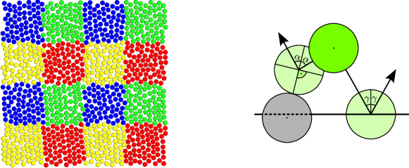
Fig. 1: Left: Scheme of the cell decomposition. To ensure independence of each thread only beads in cells with the same colors are moveable at the same time. In every sweep the checkerboard is shifted by a random vector to ensure ergodicity Right: Scheme of event chain reflections to handle cell boundary events, whenever a disk moved by an EC would move outside the current cell or hit an inactive frozen disk. The angle of reflection of the EC equals the angle of incidence.

3.3 Massively parallel MC simulation

A different approach to overcome the limitations of the local MC is to increase the number of processing units used in the simulation. As seen before, the number of CPUs commonly available in standard workstations would not suffice to increase the performance to the level reached by the EC algorithm, even if ideal scaling is assumed. However, modern GPUs can execute several thousands threads simultaneously and, therefore, allow for a massively parallel simulation accessing a limited shared memory. Such a parallelization comes with its own peculiarities, in particular, it has to be taken care that no concurrent memory changes occur.

The massively parallel MC algorithm (MPMC) by Engel et al. [21, 22] relies on the spatial decomposition into a checkerboard where four “cells” forming a $2\times 2$ square belong to one thread to ensure independent areas for each thread as in Fig. 1 (left). In every sweep the checkerboard is shifted by a random vector to ensure ergodicity and a list of all particles in each cell is created and shuffled. This step is essential to ensure detailed balance, because in every cell a fixed number $n_{m}$ of particle moves are suggested to balance the work load. A thread works on the four cells in a chosen sequential order; while working on one cell, positions of particles in the other cells are frozen. If a particle attempts to leave a cell the corresponding move is rejected.

The additional rejection lowers the effectiveness of the sampling, but due to the massive parallelization the simulation runs several orders faster than a simple sequential local MC algorithm: for optimal parameters a speed up by a factor of roughly $148$ was obtained in Ref. 22 using a TESLA K20 GPU with 2496 arithmetic logic units.

3.4 Parallel event chain algorithm

Our goal is to formulate a parallel event chain (PEC) algorithm that uses commonly available resources (4 to 16 CPUs on a current multi-processor machine) which combines aspects from the EC algorithm and the massively parallelized local MC algorithm.

For the two-dimensional hard disk system our PEC algorithm for $n$ parallel threads consists of the following steps in each MC sweep:

1. Decompose the system into $4n$ square cells; the square lattice is shifted by a random vector.

2. Form $n$ blocks of $2\times 2$ square cells (cells with different colors in Fig. 1).

3. Randomly shuffle the order of cells in the blocks (select one series of colors in Fig. 1, e.g. blue, yellow, green, red)

4. Fork into $n$ threads, each of which acts on one block.

5. Create a list with $n_{m}$ EC starting disks for each of the four cells in the block by drawing with replacement.

6. Start one EC at each of the $n_{m}$ disks in the list. While working on one cell, particle positions in the other cells are frozen. Synchronize threads when list is done and repeat for all four cells in the block.

7. Go to step 1. and generate a new decomposition.

The generalization to three-dimensional hard sphere systems is obvious.

There are two aspects that turn out to be crucial for the correctness and performance of the algorithm: (i) how the list of $n_{m}$ EC starting particles is created (with or without replacement), and (ii) how ECs are treated at the cell boundaries is important for performance.

Fig. 2: Influence of event chain starting point distribution on detailed balance. For the sake of simplicity we show a one dimensional system containing only two disks. A MC sweep then consist of two ECs ($1,\,2$): EC 1 starts at the green disk, EC 2 at the blue disk (upper row). The starting points of event chains are highlighted by a red halo. The inverse sweep (lower row) also consists of two ECs (ECs $3,\,4$). Both EC 3 and EC 4 have to start at the blue disk (the end disks of EC 1 and EC 2): Although the starting points of the sweep are distinct, for the inverse sweep the event chains need to start on the same disk. To ensure detailed balance on the sweep level both sweeps need to be suggested with the same probability. Therefore a shuffled list with distinct starting points will lead to an incorrect sampling, because the inverse sweep cannot be suggested in every case.

Regarding point (ii), we note that, in the actual EC step, the EC must not leave the cell, otherwise detailed balance and independence of the parallelly working threads are not guaranteed. This means that whenever a disk moved by an EC would move outside the current cell or hit a disk that is outside the current cell, a separate treatment is required. In both cases we think it is most effective to reflect the EC at the cell wall or an inactive frozen disk at the cell wall with the angle of incidence equal to the angle of reflection as shown in Fig. 1 (right). In this way, detailed balance is still guaranteed and no rejections are introduced. In Ref. 14, it has been proposed to reject ECs reaching the cell wall or an inactive disk at the cell wall. In principle, rejections are also suited to handle these situations but will slow down the sampling and also impair the load balance among threads.

Regarding point (i), the creation of the list of $n_{m}$ starting particles for ECs is a subtle issue. At first sight, it seems favorable to shuffle a list containing $n_{m}$ distinct particles in the cell (as in the MPMC algorithm) for a given cell decomposition. Then the maximally possible number of distinct EC starting particles is guaranteed, which seems to promise more efficient sampling. However, this use of a shuffled list of distinct starting particles violates detailed balance on the sweep level and gives rise to incorrect results (unless $n_{m}=1$). To see this we note that the inverse of an EC with displacement $\ell$ starting at disk $a$ with direction $\vec{r}$ and ending at disk $b$ is an EC with the same displacement $\ell$ and the inverse direction $-\vec{r}$ starting at $b$ and ending at $a$. For a sweep with multiple ECs starting this means that the sets of starting particles of the original and the inverse sweep need not to be permutations of each other. This is, however, what is assumed when using a shuffled list of distinct particles (and is valid for local displacement MC). For detailed balance, all $n_{m}$ starting particles have to be selected with the same equal probability among all particles in the cell. Therefore, one has to create the list of starting particles by drawing with replacement (resulting in starting particles which are not necessarily distinct). We give a simple example for a situation where this becomes relevant in Fig. 2. The different statistics – either drawing with replacement or without replacement (shuffling) – of starting particles become more relevant the larger the list length $n_{m}$ is and both list types become identical for $n_{m}=1$.

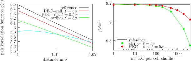
Fig. 3: Left: Influence of the validity of detailed balance on the pair correlation function $g(r)$ for several incorrect simulation variants of the EC algorithm. As a reference, we show the correct $g(r)$ as obtained from a simulation with local MC moves (black). All variants of PEC algorithms using shuffled lists of distinct EC starting particles with list length $n_{m}>1$ give incorrect results: “PEC-refl.” uses EC reflection, “PEC-rej.” uses EC rejection at the cell boundaries and a checkerboard decomposition; “stripes” uses EC rejection at the boundaries and a striped decomposition as in Ref. 14. On the other hand, all corresponding curves for algorithms with starting particle lists drawn with replacement lie strictly on top of the reference curve (and are not shown for clarity of the figure).
Right: Pressure $\beta P\sigma^{2}$ as a function of the number $n_{m}$ of started ECs per cell shuffle for different algorithms using shuffled lists for the starting particles. The colors correspond to the colors on the left. Only for $n_{m}=1$, algorithms with shuffled lists become correct and the pressure assumes the reference value.
All simulations are performed for $N=256^{2}$ disks at occupied volume fraction $\eta=0.708$.

In order to test the importance of the different statistics of starting particles for different list lengths $n_{m}$, we measure the pair correlation function $g(r)$ and obtain the pressure $P$ using eq. (4) (for a system containing $N=256^{2}$ disks at occupied volume fraction $\eta=0.708$). Finally, we compare our results with standard MC simulations with local displacement moves as a reference. We compare PEC algorithms using shuffled lists of distinct EC starting particles with PEC algorithms using lists generated by drawing particles with replacement; for both types of algorithms we consider both variants with reflection and rejection of ECs at the cell boundaries.

We find that all PEC algorithms starting $n_{m}>1$ ECs at particles drawn without replacement, i.e., by list shuffling give incorrect pair correlation functions $g(r)$. The pair correlations differ from the expected behavior for small $r\approx\sigma$ both in their functional form, see Fig. 3 (left), and in the resulting value for $P$, see Fig. 3 (right), which is obtained from the limiting value of the pair correlation at $r\rightarrow\sigma+$ according to eq. (4). Differences in the pressure $P$ increase with increasing $n_{m}$ for as shown in Fig. 3 (right). Only for the trivial list length $n_{m}=1$, i.e., with only EC started in each cell, there is no difference between a list generated by drawing with replacement and generated a list generated by shuffling, and all algorithms converge to the reference result for $P$, see Fig. 3 (right).

For all list lengths $n_{m}>1$, all PEC variants using starting particle lists generated with replacement yield the correct reference result for $g(r)$ from the local MC simulation.

We also examined the importance of replacement in the starting particle list for a parallelization of the EC algorithm through a decomposition into striped cells as proposed in Ref. [14]. Similar to the PEC with checkerboard cell decomposition we find that only drawing starting particles with replacement yields the correct pressure as also shown in Fig. 3.

The dependence of the pressure and pair correlation function on algorithmic details (choice of $\ell$, reflection/rejection, squares/stripes) for the incorrect algorithms using shuffled lists stems from the different ending point statistics of the ECs and is not easily explained on a quantitative level.

For a more extensive quantitative check of the correctness of our algorithm, we simulate a system with $N=256^{2}$ particles in the range of occupied volume fractions $\eta=0.698\ldots 0.718$, which is the regime of coexisting densities at the transition between hexatic and liquid phase as reported in Refs. 20 and 21. We compare the measured pressure with literature values from these references in Fig. 4. We find good agreement with deviations only at the highest packing fractions $\eta$, which is not a problem of our PEC algorithm itself: For large $\eta$ autocorrelation times become very large; simulations in Refs. 20 and 21 had significantly longer running times and, thus, give more accurate values.

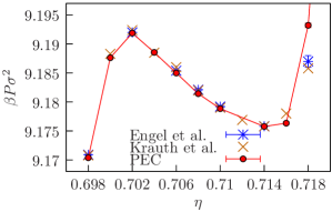
Fig. 4: Phase diagram for the liquid-hexatic transition of hard spheres. We compare the results of the three algorithms MPMC (blue, data taken from Ref. 21), sequential EC (brown, data taken from Ref. 21) and PEC (red) for a system with $N=256^{2}$ particles. Within the estimated simulation errors the algorithms yield the identical pressure density dependence. At large $\eta$, the PEC accuracy is limited by smaller running times. We run 30 independent simulations to estimate errors.

For sequential event chain implementations of hard disk systems there is a more effective way to calculate the pressure than by means of the pair correlation function and eq. (4), which uses a relation between the pressure and collision probabilities [26]. We chose to compute the pressure using the pair correlation function as this puts local MC and event chain data on the same established footing and does not imply greater computational cost because we use the pair correlation as a source of additional information on the correctness of the sampling, especially with respect to detailed balance (see Fig. 3). We suggest that the pressure calculation of Ref. 26 could be extended to PEC sampling by treating reflected event chains using a method of images and plan to explore this in future work.

4 Efficiency of the parallel event chain

To optimize the efficiency of the PEC algorithm, we can adjust the degree of parallelization $n$, the number $n_{m}$ of ECs started within each cell and the length of ECs via the total displacement length $\ell$ in the parallelization scheme. Parallelization of the EC algorithm will only offer an advantage over the sequential EC algorithm if the autocorrelation time $\tau$ in units of wall time decreases significantly with the number $n$ of threads.

First we discuss efficiency as a function of the number $n_{m}$ of ECs started within each cell. For the applications we have in mind (see below), it is favorable to use an isotropic distribution of displacement directions, which basically eliminates the striped geometry proposed in Ref. [14] because displacements transverse to the stripe direction will either be rejected or reflected with very little net displacement. To sample efficiently there should be at least one displacement per particle which suggests

$$n_{m}\sim N/4nn_{\text{EC}}\sim N\lambda_{0}/4n\ell,$$ (7)

where $n_{\text{EC}}$ denotes the average number of disks per EC. On average, this number is given by the ratio of the total displacement length $\ell$ of the EC and the mean free path of disks $\lambda_{0}$ (approximately given by the free volume per particle $\lambda_{0}\approx\sigma(\eta_{hcp}-\eta)/2\eta_{hcp}$ in the dense limit close to the close-packing density $\eta_{hcp}$),

$$n_{\text{EC}}\sim\ell/\lambda_{0}.$$ (8)

For small values of $n_{m}$, the relative fraction of wall time spent on overhead (forking / synchronizing / list creation) increases. Reducing the relative overhead by increasing $n_{m}$ leads to the saturation of speed up (in terms of the number of MC moves per wall time) by parallelization to a maximal value close to $n$ as shown in Fig. 5 (left). For values of $n_{m}$ much larger than the value (7) finite size effects will increase as each decomposition into $4n$ cells persists for a long time (in the limit $n_{m}\rightarrow\infty$ the system consists of $4n$ entirely independent smaller systems). Moreover, sampling $4n$ small cells independently for a long time is inefficient in removing large scale correlations extending over several cells. Therefore, the autocorrelation time $\tau$ of the PEC algorithm (measured in wall time) increases for large $n_{m}$ as shown in Fig. 5 (right). The optimal choice of $n_{m}$ according to the results in Fig. 5 (right) agrees with the criterion (7).

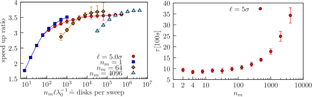
Fig. 5: Left: Ratio of the number of moves per seconds (wall time) of the parallel and sequential EC algorithm as a function of the total displacement length $\ell$ and the number $n_{m}$ of ECs started per cell configuration as a function of $n_{m}\ell/\lambda_{0}$ (for $N=256^{2}$ disks at $\eta=0.71$ using $n=4$ blocks of $2\times 2$ square cells). The speed up saturates to the maximal factor $n=4$ both for large $n_{m}$ and for large $\ell$. Since the required computation time for the synchronization overhead rises with $n_{m}$, it is more favorable to increase $\ell$ rather than $n_{m}$. The speed up should not depend on other simulation parameters such as $\eta$ or $N$.
Right: Autocorrelation time $\tau$ of the parallel EC algorithm measured in wall time as a function of the number $n_{m}$ of started ECs per cell (for $N=64^{2}$ disks at $\eta=0.704$ using $n=4$ blocks of $2\times 2$ square cells). At $n_{m}\approx 5$, each disk in a cell is moved once per sweep on average according to eq. (7). If $n_{m}$ increases the efficiency of the algorithm decreases strongly.

Now we discuss efficiency in terms of the total displacement length $\ell$ and the degree of parallelization $n$. The efficiency of the EC algorithm in general depends crucially on the average number of disks per EC $n_{\text{EC}}\sim\ell/\lambda_{0}$. In Ref. 8, it has been found that the straight EC algorithm has optimal efficiency for $\ell/\lambda_{0}\sim 10^{1}...10^{3}$ (for a system size $L\approx 34\sigma$). For smaller $\ell$, the efficiency decreases and approaches traditional local MC (corresponding to $\ell<\lambda_{0}$). For very large $\ell$, ECs comprise large parts of the system and give rise to motion similar to a collective translation of disks, which is also inefficient.

For the efficiency of the PEC algorithm, two additional competing effects are relevant to determine the optimal values for $\ell$ and the degree of parallelization $n$. On the one hand, it is obvious that the reflections at the cell walls in the PEC algorithm will impair the sampling of configuration space. Therefore, the autocorrelation time of the PEC algorithm can be significantly increased for small cell sizes, which is equivalent to small system sizes for a fixed number $4n$ of simulation cells, or for long ECs, i.e., large total displacement lengths $\ell$ of the ECs. This leads to a decrease in efficiency if the EC length $L_{\rm EC}\sim\sigma n_{\rm EC}\sim\sigma\ell/\lambda_{0}$ is increased beyond the cell size $L/2\sqrt{n}$, see Fig. 6. On the other hand, the relative overhead in computation time from parallelization (due to forking/joining/synchronizing threads) is larger for shorter chains. This leads to a decrease in efficiency for decreasing $\ell$, see Fig. 5 (left).

We conclude that $\ell$ should be chosen within the window $\ell\sim 10^{1}...10^{3}\lambda_{0}$ of optimal values for the straight EC algorithm in general, on the one hand, and as large as the cell size permits, i.e., according to $L_{\rm EC}(\ell)\sim L/2\sqrt{n}$ or

$$\ell\sim\frac{L\lambda_{0}}{\sqrt{n}\sigma}\sim\lambda_{0}\left(\frac{N}{\eta n}\right)^{1/2},$$ (9)

on the other hand. If the number $n$ of parallel threads is chosen too large, this choice for $\ell$ will drop below the optimal window $\ell<10\lambda_{0}$ for straight EC algorithms and efficiency goes down. Therefore, we propose to adjust the degree of parallelization of the PEC algorithm according to the criterion (9) rather than massively parallelize.

In Fig. 6, we quantitatively investigate the optimization of efficiency by adjusting $\ell$ or the EC length $L_{\rm EC}\sim\sigma\ell/\lambda_{0}$ according to the cell size for a degree of parallelization $n=4$. In order to investigate how much the simulation can be accelerated by parallelization with $n=4$, we measured the ratio of the autocorrelation time $\tau$ of sequential and parallel EC algorithm as a function of the number $N$ of disks for $\ell=5\sigma$ and a fixed particle density $\eta=0.71$, see Fig. 6 (left). The number $N$ of disks is related to the system size by $L=\sigma(N\pi/4\eta)^{1/2}\propto N^{1/2}$. Because we also work with a fixed number $n=4$ of threads, $N^{1/2}$ is proportional to the system size $L$ as well as the cell size $L/4$. For $\eta=0.71$, the mean free path is $\lambda_{0}\approx 0.08\sigma$ [8], such that $\ell=5\sigma$ corresponds to $\ell/\lambda_{0}\approx 62.5$, which is well within the window $\ell/\lambda_{0}\sim 10^{1}...10^{3}$ of optimal total displacement lengths for EC algorithms. In Fig. 6 (left), we show the autocorrelation time $\tau$ of the parallel and standard sequential EC algorithm in units of MC moves, where 20 MC moves correspond to one collision in the EC (using the same convention as in Ref. 8). We observe that for smaller systems $N<128^{2}$ the autocorrelation time of the parallel EC algorithm exceeds the autocorrelation time of the sequential EC algorithm. First, this means that for smaller systems $N<128^{2}$ corresponding to cell sizes $<34\sigma$ the parallelized EC algorithm becomes less efficient. Because for $\ell=5\sigma$ and $\lambda_{0}\approx 0.08\sigma$, the typical EC length is $L_{\rm EC}\sim\sigma\ell/\lambda_{0}\sim 62.5\sigma$, this marks also the range of cell sizes, which are comparable to or smaller than EC lengths. This supports our argument that EC lengths $L_{\rm EC}$ should be smaller than cell sizes for efficiency of the PEC algorithm.

The results in Fig. 6 (right) show explicitly that there exists an optimal $\ell$ for the PEC algorithm that minimizes the autocorrelation time $\tau$ for a system with $N=64^{2}$ disks. This minimum is attained for $\ell\gtrsim 10\lambda_{0}\approx 0.8$ and $\ell\approx{L\lambda_{0}}/{\sqrt{n}\sigma}\approx 1.28$ in agreement with our above arguments and criterion (9).

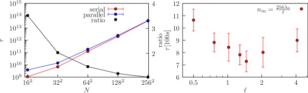
Fig. 6: Left: Autocorrelation time of the order parameter $\Psi$ for parallel and sequential EC algorithm (in units of effective local MC moves) as a function of the number of particles $N$ for fixed volume fraction $\eta=0.71$, total displacement length $\ell=5\sigma$ and one EC per cell configuration $n_{m}=1$. One collision in an EC is treated 20 effective local MC moves in a local displacement MC simulation [8]. For larger systems $N\geq 128^{2}$, the autocorrelation time differs only slightly between parallel and sequential algorithm. Therefore a good measurement for the efficiency of the algorithm is the mere increase in events per wall time shown in Fig. 5 (left).
Right: Autocorrelation time of the parallel EC algorithm (in units of wall time) as a function of the total displacement length $\ell$ and with constant number of moved disks per sweep $n_{m}n_{\text{EC}}{=}{\rm const}$ for $N=64^{2}$ and $\eta=0.704$. The autocorrelation time exhibits a minimum for $\ell\gtrsim 10\lambda_{0}\approx 0.8$ and $\ell\approx{L\lambda_{0}}/{\sqrt{n}\sigma}\approx 1.28$ in agreement with eq. (9).

Secondly, the results in Fig. 6 (left) show that for larger systems $N\geq 128^{2}$ the mere increase in MC moves per wall time is already a good measure for the efficiency of the PEC algorithm. Therefore, the ratio of the number of MC moves of the parallel and sequential EC algorithm, as shown in Fig.  5 (left) for a system of $N=256^{2}$ disks, is also a measure of efficiency. In Fig.  5 (left), we show this ratio as a function of $\ell/\sigma$ and $n_{m}$. We find that the speed up ratio is an increasing function of both $\ell$ and $n_{m}$. For large values of $\ell/\sigma$ or $n_{m}$, the speed up ratio approaches $\approx 3.9$ from below, which is remarkably close to the optimal speed up ratio $4$ for $n=4$ threads. We conclude that the PEC algorithm realizes its efficiency gain by an approximately equal autocorrelation time as the sequential EC algorithm in units of MC moves but a significant increase in the speed up ratio, i.e., the number of MC moves per wall time with the degree of parallelization $n$.

In conclusion, we propose the following strategy of choosing the degree of parallelization $n$, the total displacement $\ell$ and the number $n_{m}$ of ECs started within each cell to optimize efficiency: 1) Choose a degree of parallelization $n$ such that $N/\eta n>100$ such that $\ell>10\lambda_{0}$ according to the criterion (9). We used $n=4$ in our simulations. 2) Choose $\ell=\ell(n)$ according to the criterion (9) such that $L_{\rm EC}$ is comparable to the cell size. 3) Choose the number $n_{m}=n_{m}(n,\ell)$ according to (7).

5 Application to polymeric systems

In many applications other than pure hard core systems, we have to deal with systems containing hard core repulsion alongside with other interaction in a canonical ensemble. In Ref. 26, rejection-free extensions to the EC algorithm for continuous potentials have been presented using lifting MC moves and the concept of infinitesimal MC moves. We will use a simpler approach, where we deal with the hard core repulsion using ECs and take into account the other interactions using the standard Metropolis algorithm. As this involves rejection and, thus, a slower sampling of the hard core degrees of freedom the need for parallelization is even larger than in a gas of hard disks/spheres. We will show that EC type MC moves not only improve the sampling of dense systems but can also give rise to a physically more correct “dynamics” in an equilibrium MC simulation of dense systems.

We will apply this algorithm to a system consisting of many semiflexible polymers, such as actin filaments, which are interacting via a short-range attractive potential in a flat simulation box in three dimensions. Under the influence of this attraction, semiflexible polymers tend to form densely packed bundles. Actin filament bundles consisting of many semiflexible actin filaments, which are held together by crosslinking proteins are a realization of such a system and represent important cellular structures [27]. In vitro, F-actin bundles assemble both in the presence of crosslinking proteins and by multivalent counter ions. Theoretical work on crosslinker-mediated bundling of semiflexible polymers [28, 29, 30, 31] and counterion-mediated binding of semiflexible polyelectrolytes [32] show a discontinuous bundling transition above a threshold concentration of crosslinkers or counterions. Related bundling transitions have been found for crosslinker-mediated bundling [33], for counterion-mediated bundling [34] and for polyelectrolyte-mediated bundling [35].

It is an open question, both experimentally and theoretically, what the actual thermodynamic equilibrium state of the bundled system is and whether this state is kinetically accessible starting from a certain initial condition, for example, an unbundled polymer solution. Energetically, it is favorable to form a thick single bundle; entropically, a network of bundles (as shown in Figs. 7 B and C) might be advantageous. In both cases, the resulting bundles of semiflexible polymers are typically rather densely packed. This causes difficulties in equilibrating bundled structures in traditional MC simulations employing local moves. In Ref. 30 MC simulations showed evidence for kinetically arrested states with segregated sub-bundles, in Ref. 36 kinetically arrested bundle networks have been observed. Further numerical progress requires a faster equilibration of dense bundle structures. Ideally, the simulation reproduces the physically realistic center of mass diffusion kinetics of whole bundles. Networks of bundles have also been observed experimentally in vitro for actin bundles with crosslinkers [37] and, more recently, in actin solutions where the counterion concentration has been increased in a controlled manner [38, 39].

Here we report a first application of the EC algorithm to a polymeric system of semiflexible harmonic chains (SHC) which are modeled as chains of hard spheres or beads of diameter $\sigma$ connected by extensible springs with rest length $b_{0}=\sigma$ and spring constant $k$ with an additional three bead bending energy characterized by a bending rigidity $\kappa$ [40]. Beads in different chains also interact with a short-ranged attractive square well potential of strength $g$ and range $d$. We choose the potential strength $g$ well above the critical value for bundling [28, 30, 31]; the range of the attractive square well potential is $d=0.5\sigma$.

The energy of this system can be expressed as

$$H[{t_{i}}]=\sum_{n}\left[\kappa\sum_{i=0}^{N-2}\left(1-\frac{\vec{t}_{n,i}\,\vec{t}_{n,i+1}}{\lvert\vec{t}_{n,i}\rvert\lvert\vec{t}_{n,i+1}\rvert}\right)+\frac{k}{2}\sum_{i=0}^{N-1}\left(\frac{|\vec{t}_{n,i}|}{b_{0}}-1\right)^{2}-\sum_{\begin{subarray}{c}\langle\{n,i\},\\ \{m,j\}\rangle\end{subarray}}V_{n,m}(\lvert\vec{r}_{n,i}-\vec{r}_{m,j}\rvert)\right]\,,$$ (10)

where $\vec{t}_{n,i}=\vec{r}_{n,i+1}-\vec{r}_{n,i}$ denotes the tangent vector between the $i$th and $(i+1)$th bead of the $n$th chain and $V_{n,m}(\lvert\vec{r}_{n,i}-\vec{r}_{m,j}\rvert)$ describes the pairwise attractive square-well potential and the hard sphere condition. We present simulation results for $k=100k_{B}T$, $\kappa=20k_{B}T$ and $g=1k_{B}T$.

We consider an ensemble of many SHC in a flat box geometry of edge lengths $300\sigma\times 300\sigma\times 5\sigma$; this geometry is similar to what is used in microfluidic experimental setups in Ref. 39. For the chosen potential strength, the SHCs bind together and form a locally dense bundle resembling a dense hard sphere liquid. For systems containing many SHCs prepared in an initial state resembling a polymer solution (see Fig. 7 A), we obtain network bundle structures, which are very similar to those seen in experiments for F-actin [38, 39], see Fig. 7 B and C. A detailed quantitative investigation of these structures will follow in future publications. The network bundle structure is stationary or kinetically arrested on the accessible simulation time scales and characteristic for the initial state of a homogeneous and isotropic polymer solution as it is also used in the experiments [38, 39].

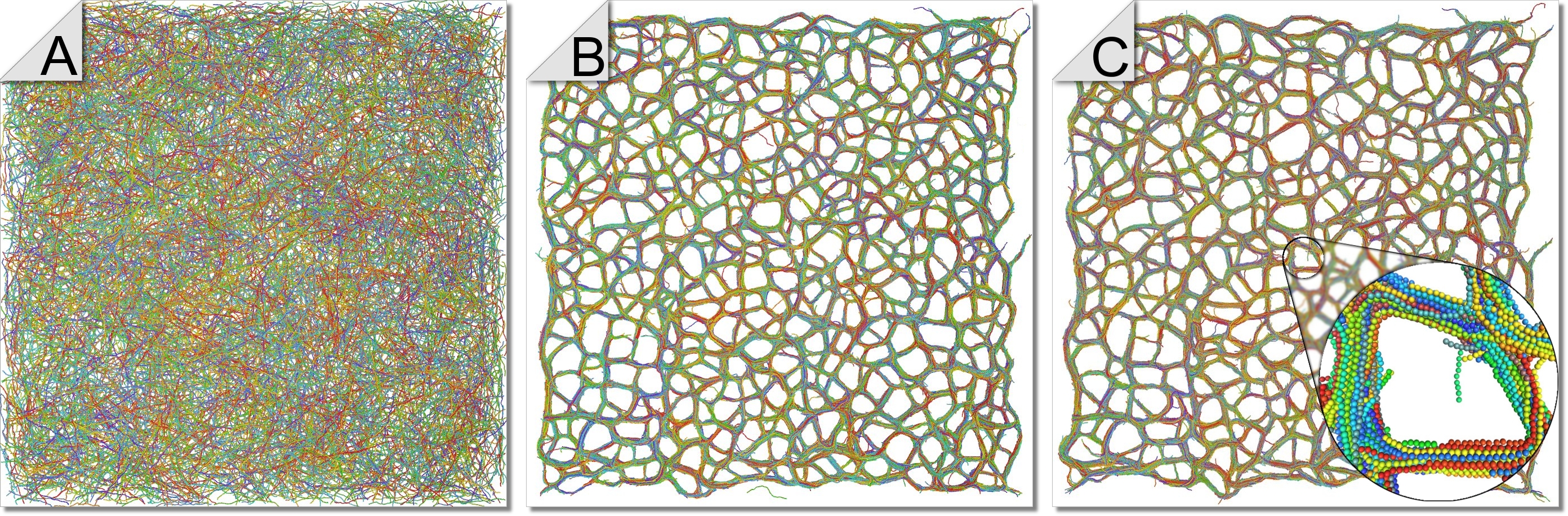
Fig. 7: Three snapshots of polymer system with $10000$ SHCs containing each $50$ beads in a flat box of edge lengths $300\sigma\times 300\sigma\times 5\sigma$ with fixed boundaries. Chain colors are arbitrary and only to distinguish different chains. The initial state A of the simulation is prepared with homogeneously and isotropically distributed chains resembling a polymer solution state. Snapshot B is taken after $3.3\cdot 10^{6}$ sweeps, snapshot C after $5.1\cdot 10^{6}$ sweeps (in each MC sweep one event chain is started on each particle). Apparently, a stationary state is reached in snapshot B.

To adapt the EC algorithm to the polymeric SHC system, the hard sphere repulsion is treated by an EC. The additional energies, such as bending, stretching and short-range inter-polymer attraction are treated conventionally employing Metropolis MC steps with rejections. First the entire EC is calculated as if we deal with a hard sphere system. After that the energy difference between the initial and final configuration determines if the whole EC move is accepted or rejected. This leads to a total displacement $\ell$ which determines the rejection rate. By adjusting the total displacement to an optimal value $\ell_{\rm opt}$, we can realize optimal acceptance rates around $50\%$.

Our first simulation results show that such a dense polymeric system can also benefit from the EC algorithm. First, we measure the diffusion coefficient $D$ for a bundle of polymers depending on the number of polymers $N_{p}$ while interpreting the number of MC sweeps as time. The overdamped time evolution of the bundle (neglecting hydrodynamic effects) is described by Rouse dynamics, which gives a diffusion coefficient decreasing as $D\sim N_{p}^{-1}$ [41]. Applying single displacement local MC moves to such a system leads to an unphysically slow diffusion behavior with $D\sim N_{p}^{-1.2}$, while the EC algorithm leads to the correct behavior of the diffusion constant as shown in Fig. 8. This implies that the event chain as a cluster move not only allows for a more efficient sampling in this system, but also incorporates some essential features of the true dynamics, in that it allows (at least on a coarse scale) for an identification of “Monte Carlo time” (number of performed sweeps) and physical time. For the extraction of quantitative information a gauge would be needed, e.g. an otherwise measured (experiment, MD simulation) diffusion constant. The range $d$ of the attractive square well potential is $d=0.5\sigma$ and, therefore, rather large compared to the mean free path of densely packed disks examined before. For smaller potential ranges $d$ we expect the bundle diffusion to exhibit a stronger slow down without EC moves.

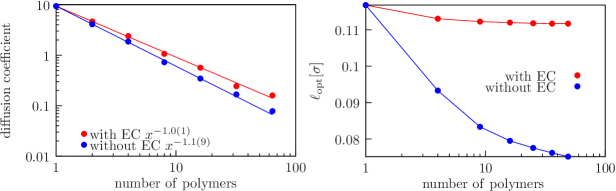
Fig. 8: Left: Diffusion constant of the center of mass of a polymer bundle consisting of $N_{p}$ polymers. Using an EC algorithm, the result $D\sim N_{p}^{-1}$ characteristic for Rouse dynamics is reproduced, which allows for an identification of “Monte Carlo time” as physical time. Right: “Optimal move” length $\ell_{\text{opt}}$ determined by adjusting the rejection rate to $0.5$ as a function of the number $N_{p}$ of polymers in a bundle. The acceptance probability is not reduced by the number of polymers if the event chain algorithm is used. This leads to a more effective sampling.

Furthermore we determine how the optimal displacement length $\ell_{\text{opt}}$ depends on the number $N_{p}$ of polymers in a bundle. For an efficient simulation, $\ell_{\text{opt}}$ should not depend on the thickness of a bundle. Figure 8 shows that $\ell_{\text{opt}}$ is drastically decreasing with $N_{p}$ for local single displacement MC moves, whereas it is almost independent of $N_{p}$ for the EC algorithm. For smaller potential ranges $d$ we expect a faster decrease in $\ell_{\text{opt}}$. Again, we expect the decrease to be much stronger without EC moves.

These two results can be interpreted such that local single displacement moves do not produce a realistic Rouse dynamics including center of mass diffusion of whole bundles and do not allow to interpret the MC sweep number as a realistic time. Furthermore, first simulations suggest that even if the EC length is not much longer than a single displacement the speed up in equilibration time can be very high.

With the parallelized version of the EC algorithm it is possible to reach a stationary quasi-equilibrium state for large system sizes as shown in Fig.  7, which allows us to compare with experimental systems. The snapshot exhibits the same bundle network features as observed in experiments [38, 39], namely the formation of a network of bundles as the final state of the aggregation process. The network exhibits a polygonal cell structure, which is also observed in Refs. 38, 39. Further quantitative comparison between simulation and experiments will be performed in future investigations. The efficient sampling technique using the PEC will be useful to adress the question whether the experimentally observed network states are true equilibrium states (due to their higher entropy in comparison to the energetically favorable single bundle) or are kinetically trapped metastable states and how the formation of a network depends on the global parameters (such as density and contour lengths of the polymer chains) and initial conditions.

6 Conclusion

We presented a parallelization scheme for the EC algorithm and performed extensive tests for correctness and efficiency for the hard sphere system in two dimensions.

For parallelization we use a spatial partitioning approach into simulation cells. We find that it is crucial for correctness of the PEC algorithm that the starting particles for ECs in each sweep are drawn with replacement. We have shown implementations without replacement to give incorrect results for the pair correlation function and the resulting pressure, see Figs. 3. The reason for this incorrect results is the violation of detailed balance on the sweep level.

We analyzed the performance gains for the PEC algorithm and find the criterion (9) for an optimal degree of parallelization. Because of the cluster nature of EC moves massive parallelization will not be optimal. The PEC algorithm will therefore be best suited for commonly available multicore CPUs with shared memory.

Finally, we discussed a first application of the algorithm to dense polymer systems. Using ECs we simulated bundle formation in a solution of attractive semiflexible polymers. The EC moves give rise to a faster and much more realistic bundle diffusion behavior. This allows us to simulate large systems, in particular, if the EC algorithm is parallelized. The simulation exhibits large-scale network bundle structures, see Fig. 7, which are very similar to structures observed in recent experiments [38, 39].

References

- [1] N. Metropolis, A. Rosenbluth, M. Rosenbluth, A. Teller, E. Teller, Equation of State Calculations by Fast Computing Machines, J. Chem. Phys. 21 (6) (1953) 1087.
- [2] R. Swendsen, J.-s. Wang, Nonuniversal Critical Dynamics in Monte Carlo Simulations, Phys. Rev. Lett. 58 (2) (1987) 86–88.
- [3] U. Wolff, Collective Monte Carlo Updating for Spin Systems, Phys. Rev. Lett. 62 (4) (1989) 361–364.
- [4] C. Dress, W. Krauth, Cluster Algorithm for Hard Spheres and Related Systems, J. Phys. A: Math. and Gen. 28 (23) (1995) L597–L601.
- [5] A. Buhot, W. Krauth, Numerical Solution of Hard-Core Mixtures, Phys. Rev. Lett. 80 (17) (1998) 3787–3790.
- [6] L. Santen, W. Krauth, Absence of Thermodynamic Phase Transition in a Model Glass Former, Nature 405 (6786) (2000) 550–1.
- [7] J. Liu, E. Luijten, Rejection-Free Geometric Cluster Algorithm for Complex Fluids, Phys. Rev. Lett. 92 (3) (2004) 035504.
- [8] E. P. Bernard, W. Krauth, D. B. Wilson, Event-Chain Monte Carlo Algorithms for Hard-Sphere Systems, Phys. Rev. E 80 (2009) 056704.
- [9] J. A. Anderson, C. D. Lorenz, A. Travesset, General Purpose Molecular Dynamics Simulations Fully Implemented on Graphics Processing Units, J. Comput. Phys. 227 (10) (2008) 5342–5359.
- [10] J. van Meel, A. Arnold, D. Frenkel, S. Portegies Zwart, R. Belleman, Harvesting Graphics Power for MD simulations, Mol. Sim. 34 (3) (2008) 259–266.
- [11] T. Preis, P. Virnau, W. Paul, J. J. Schneider, GPU accelerated Monte Carlo simulation of the 2D and 3D Ising Model, J. Comput. Phys. 228 (12) (2009) 4468–4477.
- [12] Y. Komura, Y. Okabe, GPU-based Swendsen–Wang Multi-Cluster Algorithm for the Simulation of Two-Dimensional Classical Spin Systems, Comput. Phys. Comm. 183 (6) (2012) 1155–1161.
- [13] Y. Komura, Y. Okabe, CUDA programs for the GPU computing of the Swendsen–Wang multi-cluster spin flip algorithm: 2D and 3D Ising, Potts , and XY models, Comput. Phys. Comm. 185 (3) (2014) 1038–1043.
- [14] S. C. Kapfer, W. Krauth, Sampling from a Polytope and Hard-Disk Monte Carlo, in: J. Phys.: Conf. Ser., Vol. 454, IOP Publishing, 2013, p. 012031.
- [15] K. Strandburg, Two-Dimensional Melting, Rev. Mod. Phys. 60 (1) (1988) 161–207.
- [16] J. M. Kosterlitz, D. J. Thouless, Ordering, Metastability and Phase Transitions in Two-Dimensional Systems, J. Phys. C 6 (7) (1973) 1181.
- [17] B. Halperin, D. Nelson, Theory of Two-Dimensional Melting, Phys. Rev. Lett. 41 (2) (1978) 121–124.
- [18] A. Young, Melting and the Vector Coulomb Gas in Two Dimensions, Phys. Rev. B 19 (4) (1979) 1855–1866.
- [19] C. Mak, Large-scale Simulations of the Two-dimensional Melting of Hard Disks, Phys. Rev. E 73 (6) (2006) 065104.
- [20] E. P. Bernard, W. Krauth, Two-Step Melting in Two Dimensions: First-Order Liquid-Hexatic Transition, Phys. Rev. Lett. 107 (2011) 155704.
- [21] M. Engel, J. A. Anderson, S. C. Glotzer, M. Isobe, E. P. Bernard, W. Krauth, Hard-disk Equation of State: First-order Liquid-Hexatic Transition in Two Dimensions with Three Simulation Methods, Phys. Rev. E 87 (2013) 042134.
- [22] J. A. Anderson, E. Jankowski, T. L. Grubb, M. Engel, S. C. Glotzer, Massively Parallel Monte Carlo for Many-Particle Simulations on GPUs, J. Comput. Phys. 254 (2013) 27–38.
- [23] M. De Berg, M. Van Kreveld, M. Overmars, O. C. Schwarzkopf, Computational Geometry, Springer, Berlin, 2000.
- [24] Cgal, Computational Geometry Algorithms Library, http://www.cgal.org.
- [25] G. O. Roberts, A. Gelman, W. R. Gilks, et al., Weak Convergence and Optimal Scaling of Random Walk Metropolis Algorithms, Ann. Appl. Probab. 7 (1) (1997) 110–120.
- [26] M. Michel, S. C. Kapfer, W. Krauth, Generalized Event-Chain Monte Carlo: Constructing RejectionFree Global-Balance Algorithms from Infinitesimal Steps, J. Chem. Phys. 140 (2014) 054116.
- [27] J. R. Bartles, Parallel Actin Bundles and their Multiple Actin-Bundling Proteins, Curr. Opin. Cell Biol. 12 (1) (2000) 72–78.
- [28] J. Kierfeld, R. Lipowsky, Unbundling and Desorption of Semiflexible Polymers, Europhys. Lett. 62 (2) (2003) 285–291.
- [29] J. Kierfeld, R. Lipowsky, Duality Mapping and Unbinding Transitions of Semiflexible and Directed Polymers, J. Phys. A: Math. Gen. 38 (9) (2005) L155–L161.
- [30] J. Kierfeld, T. Kühne, R. Lipowsky, Discontinuous Unbinding Transitions of Filament Bundles, Phys. Rev. Lett. 95 (3) (2005) 038102.
- [31] T. A. Kampmann, H.-H. Boltz, J. Kierfeld, Controlling Adsorption of Semiflexible Polymers on Planar and Curved Substrates, J. Chem. Phys. 139 (3) (2013) 034903.
- [32] I. Borukhov, R. Bruinsma, W. Gelbart, A. Liu, Elastically Driven Linker Aggregation between Two Semiflexible Polyelectrolytes, Phys. Rev. Lett. 86 (10) (2001) 2182–2185.
- [33] P. Benetatos, E. Frey, Depinning of Semiflexible Polymers, Phys. Rev. E 67 (5) (2003) 051108.
- [34] B. Shklovskii, Wigner Crystal Model of Counterion Induced Bundle Formation of Rodlike Polyelectrolytes, Phys. Rev. Lett. 82 (16) (1999) 3268–3271.
- [35] J. DeRouchey, R. R. Netz, J. O. Rädler, Structural Investigations of DNA-Polycation Complexes, Eur. Phys. J. E 16 (1) (2005) 17–28.
- [36] M. J. Stevens, Bundle Binding in Polyelectrolyte Solutions, Phys. Rev. Lett. 82 (1) (1999) 101–104.
- [37] O. Pelletier, E. Pokidysheva, L. S. Hirst, N. Bouxsein, Y. Li, C. R. Safinya, Structure of Actin Cross-Linked with -Actinin: A Network of Bundles, Phys. Rev. Lett. 91 (14) (2003) 148102.
- [38] F. Huber, D. Strehle, J. Käs, Counterion-Induced Formation of Regular Actin Bundle Networks, Soft Matter 8 (4) (2012) 931–936.
- [39] S. Deshpande, T. Pfohl, Hierarchical Self-Assembly of Actin in Micro-Confinements using Microfluidics, Biomicrofluidics 6 (3) (2012) 034120.
- [40] J. Kierfeld, O. Niamploy, V. Sa-yakanit, R. Lipowsky, Stretching of Semiflexible Polymers with Elastic Bonds, Eur. Phys. J. E 14 (1) (2004) 17–34.
- [41] M. Doi, S. Edwards, The Theory of Polymer Dynamics, Clarendon Press, Oxford, 1986.