Rigorous approximation of diffusion coefficients for expanding maps

Abstract.

We use Ulam’s method to provide rigorous approximation of diffusion coefficients for uniformly expanding maps. An algorithm is provided and its implementation is illustrated using Lanford’s map.

1. Introduction

The use of computers is essential for predicting and understanding the behaviour of many physical systems. Sensitive dependence on initial conditions is typical in many physical systems. This sensitivity problem raises nontrivial reliability and stability issues regarding any computational approach to such systems. Moreover, it strongly motivates the study of reliable computational methods for understanding statistical properties of physical systems.

In this note we consider the rigorous computation of diffusion coefficients in a class of systems where a central limit theorem holds. Such coefficients are focal in the study of limit theorems and fluctuations for dynamical systems (see [8, 12, 13, 17, 23, 28] and references therein). Given a piecewise expanding map, an observable, and a pre-specified tolerance on error, we approximate in a certified way the diffusion coefficient up to the per-specified error (see Theorem 2.3).

Our rigorous approximation is based on a suitable finite dimensional approximation (discretization) of the system, called Ulam’s method [36]. Ulam’s method is known to provide rigorous approximations of SRB (Sinai-Ruelle-Bowen) measures and other important dynamical quantities for different types of dynamical systems (see [1, 2, 3, 9, 10, 25, 14, 15, 29, 30] and references therein). Moreover, this method was also used to detect coherent structures in geophysical systems (see e.g. [34], [7]).

In [32], following the approach of [18], a Fourier approximation scheme was used to estimate diffusion coefficients for expanding maps. The approach of [32] requires the map to have a Markov partition and to be piecewise analytic. Although the result of [32] provides an order of convergence, it does not compute the constant hiding in the rate of convergence. In our approach, we do not require the map to admit a Markov partition and we only assume it is piecewise $C^{2}$. More importantly, our approximation is rigorous. To give the reader a flavour of what we mean by rigorous, we close this section by providing in part (b) of the following theorem a prototype result of this paper:

Theorem 1.1.

Let

(1.1) $$T(x)=2x+\frac{1}{2}x(1-x)\hskip 14.22636pt{\text{(mod }1)}.$$

1. $T$ admits a unique absolutely continuous invariant measure $\nu$ and if $\psi$ is a function of bounded variation the Central Limit Theorem holds:

   $$\frac{1}{\sqrt{n}}\left(\sum_{i=0}^{n-1}\psi(T^{i}x)-n\int_{I}\psi d\nu\right){\overset{\text{law}}{\longrightarrow}}\mathcal{N}(0,\sigma^{2}).$$

2. For $\psi=x^{2}$ the diffusion coefficient $\sigma^{2}\in[0.3458,0.4152]$.

In Section 2, we first introduce our framework and the assumptions on it. We then state the problem and introduce the method of approximation. The statement of the general results (Theorem 2.3 and Theorem 2.5) and an application to expanding maps with a neutral fixed point are also included in Section 2. Section 3 contains the proofs and an algorithm. Section 4 contains an example, using Lanford’s map, that illustrates the implementation of the algorithm of Section 3 and proves part (b) of Theorem 1.1.

2. The setting

2.1. The system and its transfer operator

Let $(I,\mathcal{B},m)$ be the measure space, where $I:=[0,1]$, $\mathcal{B}$ is Borel $\sigma$-algebra, and $m$ is the Lebesgue measure on $I$. Let $T:I\rightarrow I$ be piecewise $C^{2}$ and expanding (see [22, 31] for original references and [6] for a profound background on such systems). The transfer operator (Perron-Frobenius) [4] associated with $T$, $P:L^{1}\rightarrow L^{1}$ is defined by duality: for $f\in L^{1}$ and $g\in L^{\infty}$

$$\int_{I}f\cdot g\circ Tdm=\int_{I}P(f)\cdot gdm.$$

Moreover, for $f\in L^{1}$ we have

$$Pf(x)=\sum_{y=T^{-1}x}\frac{f(y)}{|T^{\prime}(y)|}.$$

For $f\in L^{1}$, we define

$$Vf=\inf_{\overline{f}}\{\text{var}\overline{f}\,:f=\overline{f}\text{ a.e.}\},$$

where

$$\text{var}\overline{f}=\sup\{\sum_{i=0}^{l-1}|\overline{f}(x_{i+1})-\overline{f}(x_{i})|\,:0=x_{0}<x_{1}<\dots<x_{l}=1\}.$$

We denote by $BV$ the space of functions of bounded variation on $I$ equipped with the norm $||\cdot||_{BV}=V(\cdot)+||\cdot||_{1}$. Further, we introduce the mixed operator norm which will play a key role in our approximation:

$$|||P|||=\underset{||f||_{BV}\leq 1}{\sup}||Pf||_{1}.$$

2.2. Assumptions

We assume:
(A1) $\exists\,\ \alpha\in(0,1)$, and $B_{0}\geq 0$ such that $\forall f\in BV$

$$VPf\leq\alpha Vf+B_{0}||f||_{1};$$

(A2) $P$, as operator on $BV$, has $1$ as a simple eigenvalue. Moreover $P$ has no other eigenvalues whose modulus is unity.

Remark 2.1.

It is important to remark that the constants $\alpha$ and $B_{0}$ in (A1) depend only on the map $T$ and have explicit analytic expressions (see [22]).

The above assumptions imply that $T$ admits a unique absolutely continuous invariant measure $\nu$, such that $\frac{d\nu}{dm}:=h\in BV$. Moreover, the system $(I,\mathcal{B},\nu,T)$ is mixing and it enjoys exponential decay of correlations for observables in $BV$ (see [4] for a profound background on this topic).

2.3. The problem

Let $\psi\in BV$ and define

(2.1) $$\sigma^{2}:=\lim_{n\to\infty}\frac{1}{n}\int_{I}\left(\sum_{i=0}^{n-1}\psi(T^{i}x)-n\int_{I}\psi d\nu\right)^{2}d\nu.$$

Under our assumptions the limit in (2.1) exists (see [12]), and by using the summability of the correlation decay and the duality property of $P$, one can rewrite $\sigma^{2}$ as

(2.2) $$\sigma^{2}:=\int_{I}\hat{\psi}^{2}hdm+2\sum_{i=1}^{\infty}\int_{I}P^{i}(\hat{\psi}h)\hat{\psi}dm,$$

where

$$\hat{\psi}:=\psi-\mu\text{ and }\mu:=\int_{I}\psi d\nu.$$

The number $\sigma^{2}$ is called the variance, or the diffusion coefficient, of $\sum_{i=0}^{n-1}\psi(T^{i}x)$. In particular, for the systems under consideration, it is well known (see [12]) that the Central Limit Theorem holds:

$$\frac{1}{\sqrt{n}}\left(\sum_{i=0}^{n-1}\psi(T^{i}x)-n\int_{I}\psi d\nu\right){\overset{\text{law}}{\longrightarrow}}\mathcal{N}(0,\sigma^{2}).$$

Moreover, $\sigma^{2}>0$ if and only if $\psi\not=c+\phi\circ T-\phi$, $\phi\in BV$, $c\in\mathbb{R}$.

The goal of this paper is to provide an algorithm whose output approximates $\sigma^{2}$ with rigorous error bounds. The first step in our approach will be to discretize $P$ as follows:

2.4. Ulam’s scheme

Let $\eta:=\{I_{k}\}_{k=1}^{d(\eta)}$ be a partition of $[0,1]$ into intervals of size $\lambda(I_{k})\leq\varepsilon$. Let $\mathfrak{B}_{\eta}$ be the $\sigma$-algebra generated by $\eta$ and for $f\in L^{1}$ define the projection

$$\Pi_{\varepsilon}f=E(f|\mathfrak{B}_{\eta}),$$

and

$$P_{\varepsilon}=\Pi_{\varepsilon}\circ P\circ\Pi_{\varepsilon}.$$

$P_{\varepsilon}$, which is called Ulam’s approximation of $P$, is finite rank operator which can be represented by a (row) stochastic matrix acting on vectors in $\mathbb{R}^{d(\eta)}$ by left multiplication. Its entries are given by

$$P_{kj}=\frac{\lambda(I_{k}\cap T^{-1}(I_{j}))}{\lambda(I_{k})}.$$

The following lemma collects well known results on $P_{\varepsilon}$. See for instance [25] for proofs of (1)-(4) of the lemma, and [25, 15] and references therein for statement (5) of the lemma.

Lemma 2.2.

For $f\in BV$ we have

1. $V(\Pi_{\varepsilon}f)\leq V(f)$;

2. $||f-\Pi_{\varepsilon}f||_{1}\leq\varepsilon V(f)$;

3. $$VP_{\varepsilon}f\leq\alpha Vf+B_{0}||f||_{1},$$

   where $\alpha$ and $B_{0}$ are the same constants that appear in (A1);

4. $|||P_{\eta}-P|||\leq\Gamma\varepsilon,$ where $\Gamma=\max\{\alpha+1,B_{0}\}$;

5. $P_{\varepsilon}$ has a unique fixed point $h_{\varepsilon}\in BV$. Moreover, $\exists$ a computable constant $K_{*}$ such that

   $$||h_{\varepsilon}-h||_{1}\leq K_{*}\varepsilon\ln\varepsilon^{-1}.$$

   In particular, for any $\tau>0$, there exists $\varepsilon_{*}$ such that $||h_{\varepsilon_{*}}-h||_{1}\leq\tau$.

2.5. Statement of the general result

Define

$$\hat{\psi}_{\varepsilon}:=\psi-\mu_{\varepsilon}\text{ and }\mu_{\varepsilon}:=\int_{I}\psi h_{\varepsilon}dm.$$

Set

$$\sigma^{2}_{\varepsilon,l}:=\int_{I}\hat{\psi}_{\varepsilon}^{2}h_{\varepsilon}dm+2\sum_{i=1}^{l-1}\int_{I}P_{\varepsilon}^{i}(\hat{\psi}_{\varepsilon}h_{\varepsilon})\hat{\psi}_{\varepsilon}dm.$$

Theorem 2.3.

For any $\tau>0$, $\exists$ $l_{*}>0$ and $\varepsilon_{*}>0$ such that

$$|\sigma^{2}_{\varepsilon_{*},l_{*}}-\sigma^{2}|\leq\tau.$$

Remark 2.4.

Theorem 2.3 says that given a pre-specified tolerance on error $\tau>0$, one finds $l_{*}>0$ and $\varepsilon_{*}>0$ so that $\sigma^{2}_{\varepsilon_{*},l_{*}}$ approximates $\sigma$ up to the pre-specified error $\tau$. In subsection 3.1 we provide an algorithm that can be implemented on a computer to find $l_{*}$ and $\varepsilon_{*}$, and consequently $\sigma^{2}_{\varepsilon_{*},l_{*}}$.

To illustrate the issue of the rate of convergence and to elaborate on why we define the approximate diffusion by $\sigma^{2}_{\varepsilon,l}$ as a truncated sum, let us define

$$\sigma^{2}_{\varepsilon}:=\int_{I}\hat{\psi}_{\varepsilon}^{2}h_{\varepsilon}dm+2\sum_{i=1}^{\infty}\int_{I}P_{\varepsilon}^{i}(\hat{\psi}_{\varepsilon}h_{\varepsilon})\hat{\psi}_{\varepsilon}dm.$$

Theorem 2.5.

$\exists$ a computable constant $\tilde{K}_{*}$ such that

$$|\sigma^{2}_{\varepsilon}-\sigma^{2}|\leq\tilde{K}_{*}\varepsilon(\ln\varepsilon^{-1})^{2}.$$

Remark 2.6.

Note that $\sigma_{\varepsilon}^{2}$ can be written as

(2.3) $$\begin{split}\sigma^{2}_{\varepsilon}&=\int_{I}\hat{\psi}_{\varepsilon}^{2}h_{\varepsilon}dm+2\sum_{i=1}^{\infty}\int_{I}P_{\varepsilon}^{i}(\hat{\psi}_{\varepsilon}h_{\varepsilon})\hat{\psi}_{\varepsilon}dm\\ &=-\int_{I}\hat{\psi}_{\varepsilon}^{2}h_{\varepsilon}+2\int_{I}\hat{\psi}_{\varepsilon}({\bf 1}-P_{\varepsilon})^{-1}(\hat{\psi}_{\varepsilon}h_{\varepsilon})dm.\end{split}$$

Since $P_{\varepsilon}$ has a matrix representation, and consequently $(I-P_{\varepsilon})^{-1}$ is a matrix, one may think that $\sigma^{2}_{\varepsilon}$ provides a more sensible formula to approximate $\sigma^{2}$ than $\sigma^{2}_{\varepsilon,l}$. However, from the rigorous computational point of view one has to take into account the errors that arise at the computer level when estimating $(I-P_{\varepsilon})^{-1}$. Indeed $(I-P_{\varepsilon})^{-1}$ can be computed rigorously on the computer by estimating it by a finite sum plus an error term coming from estimating the tail of the sum. This is what we do in Theorem 2.3.

Remark 2.7.

In [5] an example of a highly regular expanding map (piecewise affine) was presented where the exact rate of Ulam’s method for approximating the invariant density $h$ is $\varepsilon\ln\varepsilon^{-1}$. In Theorem 2.5 the rate for approximating $\sigma^{2}$ is $\varepsilon(\ln\varepsilon^{-1})^{2}$. This is due to the fact that $||h-h_{\varepsilon}||_{1}$ is an essential part in estimating $\sigma^{2}$ and the extra $\ln\varepsilon^{-1}$ appears because of the infinite sum in the formula of $\sigma^{2}$.

Remark 2.8.

By using the representation (2.3) of $\sigma_{\varepsilon}^{2}$, it is obvious that the main task in the proof of Theorem 2.5 is to estimate

$$|||({\bf 1}-P)^{-1}-({\bf 1}-P_{\varepsilon})^{-1}|||_{BV_{0}\to L^{1}},$$

where $BV_{0}=\{f\in BV\text{ s.t.}\int fdm=0\}$. Thus, it would be tempting to use estimate (9) in Theorem 1 of [19], which reads:

(2.4) $$\begin{split}&|||({\bf 1}-P)^{-1}-({\bf 1}-P_{\varepsilon})^{-1}|||_{BV_{0}\to L^{1}}\\ &\hskip 71.13188pt\leq|||P-P_{\varepsilon}|||_{BV_{0}\to L^{1}}^{\theta}(c_{1}||({\bf 1}-P_{\varepsilon})^{-1}||_{BV_{0}}+c_{2}||({\bf 1}-P_{\varepsilon})^{-1}||_{BV_{0}}^{2}),\end{split}$$

where $\theta=\frac{\ln(r/\alpha)}{\ln(1/\alpha)}$, $r\in(\alpha,1)$, and $c_{1},c_{2}$ are constants that dependent only on $\alpha$, $B_{0}$ and $r$. On the one hand, this would lead to a shorter proof than the one we present in section 3; however, estimate (2.4) would lead to a convergence rate of order $\varepsilon^{\theta}$, where $0<\theta<1$ which is slower than the rate obtained in Theorem 2.5. Naturally, this have led us to opt for using the proofs of section 3.

2.6. Approximating the diffusion coefficient for non-uniformly expanding maps

We now show that Theorem 2.3 can be used to approximate the diffusion coefficient for non-uniformly expanding maps. We restrict the presentation to the model that was popularized by Liverani-Saussol-Vaienti [27]. Such systems have attracted the attention of both mathematicians [27, 37] and physicists because of their importance in the study of intermittent transition to turbulence [33]. Let

(2.5) $$S(x)=\begin{cases}x(1+2^{\gamma}x^{\gamma})\quad x\in[0,\frac{1}{2}]\\ 2x-1\quad\quad\quad x\in(\frac{1}{2},1]\end{cases},$$

where the parameter $\gamma\in(0,1)$. $S$ has a neutral fixed point at $x=0$. It is well known that $S$ admits a unique absolutely continuous probability measure $\tilde{\nu}$, and the system enjoys polynomial decay of correlation for Hölder observables [37]. For $\gamma\in(0,\frac{1}{2})$ it is known that the system satisfies the Central Limit Theorem. To study such systems it is often useful to first induce $S$ on a subset of $I$ where the induced map $T$ is uniformly expanding. In particular for the map (2.5), denoting its first branch by $S_{1}$ and the second one by $S_{2}$, one can induce $S$ on $\Delta:=[\frac{1}{2},1]$. For $n\geq 0$ we define

$$x_{0}:=\frac{1}{2}\text{ and }x_{n+1}=S_{1}^{-1}(x_{n}).$$

Set

$$W_{0}:=(x_{0},1),\text{and }W_{n}:=(x_{n},x_{n-1}),\,n\geq 1.$$

For $n\geq 1$, we define

$$Z_{n}:=S_{2}^{-1}(W_{n-1}).$$

Then we define the induced map $T:\Delta\to\Delta$ by

(2.6) $$T(x)=S^{n}(x)\text{ for $x\in Z_{n}$.}$$

Observe that

$$S(Z_{n})=W_{n-1}\text{ and }R_{Z_{n}}=n,$$

where $R_{Z_{n}}$ is the first return time of $Z_{n}$ to $\Delta$. For $x\in\Delta$, we denote by $R(x)$ the first return time of $x$ to $\Delta$. Let $f$ be Hölder with $\int_{I}fd\tilde{\nu}=0$. Then diffusion coefficient of the system $S$ can be written using the data of the induced map $T$ (see [17]). In particular, for $x\in\Delta$, writing $\psi(x)=\sum_{i=0}^{R(x)-1}f(S^{i}x)$, the diffusion coefficient is given by

$$\sigma^{2}:=\int_{\Delta}\psi^{2}hdm_{\Delta}+2\sum_{i=1}^{\infty}\int_{\Delta}P^{i}(\psi h)\psi dm_{\Delta},$$

where $h$ is the unique invariant density of induced map $T$, $P$ is the Perron-Frobenius operator associated with $T$, and $m_{\Delta}$ is normalized Lebesgue measure on $\Delta$. Thus, for $\psi\in BV$ one can use, Theorem 2.3 to approximate $\sigma^{2}$.

3. Proofs and an Algorithm

We first prove two lemmas that will be used to prove Theorem 2.3. The explicit estimates of Lemma 3.2 below will also be used in Subsection 3.1 where we present our algorithm to rigorously estimate diffusion coefficients.

Lemma 3.1.

For $\psi\in BV$, we have

1. $||\hat{\psi}||_{\infty}\leq 2||\psi||_{\infty}$ and $||\hat{\psi}_{\varepsilon}||_{\infty}\leq 2||\psi||_{\infty}$;

2. $|\int_{I}(\hat{\psi}^{2}h-\hat{\psi}_{\varepsilon}^{2}h_{\varepsilon})dm|\leq 8||\psi||_{\infty}^{2}||h_{\varepsilon}-h||_{1}.$

Proof.

Using the definition of $\hat{\psi}$, $\hat{\psi}_{\varepsilon}$ we get (1). We now prove (2). We have

(3.1) $$\begin{split}|\int_{I}(\hat{\psi}^{2}_{\varepsilon}-\hat{\psi}^{2})hdm|=&|\int_{I}(\hat{\psi}_{\varepsilon}-\hat{\psi})(\hat{\psi}_{\varepsilon}+\hat{\psi})hdm|=|\int_{I}(\mu-\mu_{\varepsilon})(2\psi-\mu-\mu_{\varepsilon})hdm|\\ &\leq 4||\psi||_{\infty}|\mu_{\varepsilon}-\mu|\int_{I}hdm\leq 4||\psi||_{\infty}^{2}||h_{\varepsilon}-h||_{1}.\end{split}$$

We now use (1) and (3.1) to get

$$\begin{split}|\int_{I}(\hat{\psi}^{2}h-\hat{\psi}_{\varepsilon}^{2}h_{\varepsilon})dm|&\leq|\int_{I}(\hat{\psi}^{2}h-\hat{\psi}_{\varepsilon}^{2}h)dm|+|\int_{I}(\hat{\psi}_{\varepsilon}^{2}h-\hat{\psi}_{\varepsilon}^{2}h_{\varepsilon})dm|\\ &\leq 8||\psi||_{\infty}^{2}||h_{\varepsilon}-h||_{1}.\end{split}$$

∎

Lemma 3.2.

For any $l\geq 1$ we have

$$\begin{split}&|\sum_{i=1}^{l-1}\int_{I}\left(P^{i}_{\varepsilon}(\hat{\psi}_{\varepsilon}h_{\varepsilon})\hat{\psi}_{\varepsilon}-P^{i}(\hat{\psi}h)\hat{\psi}\right)dm|\leq 8(l-1)\cdot||\psi||^{2}_{\infty}\cdot||h_{\varepsilon}-h||_{1}\\ &+2||\psi||_{\infty}|||P_{\varepsilon}-P|||\sum_{i=1}^{l-1}\sum_{j=0}^{i-1}\left(2||\psi||_{\infty}(B_{j}+1+\frac{\alpha^{j}B_{0}}{1-\alpha})+\frac{\alpha^{j}(B_{0}+1-\alpha)}{1-\alpha}V\psi\right),\end{split}$$

where $B_{j}=\sum_{k=0}^{j-1}\alpha^{k}B_{0}.$

Proof.

$$\begin{split}&|\sum_{i=1}^{l-1}\int_{I}\left(P^{i}_{\varepsilon}(\hat{\psi}_{\varepsilon}h_{\varepsilon})\hat{\psi}_{\varepsilon}-P^{i}(\hat{\psi}h)\hat{\psi}\right)dm|\\ &\leq|\sum_{i=1}^{l-1}\int_{I}\left(P^{i}_{\varepsilon}(\hat{\psi}_{\varepsilon}h_{\varepsilon})\hat{\psi}_{\varepsilon}-P^{i}_{\varepsilon}(\hat{\psi}h)\hat{\psi}\right)dm|+|\sum_{i=1}^{l-1}\int_{I}\left(P^{i}_{\varepsilon}(\hat{\psi}h)\hat{\psi}-P^{i}(\hat{\psi}h)\hat{\psi}\right)dm|\\ &\leq|\sum_{i=1}^{l-1}\int_{I}P^{i}_{\varepsilon}(\hat{\psi}_{\varepsilon}h_{\varepsilon}-\hat{\psi}h)\psi dm|+|\sum_{i=1}^{l-1}\int_{I}\left(P^{i}_{\varepsilon}(\hat{\psi}_{\varepsilon}h_{\varepsilon})\mu_{\varepsilon}-P^{i}_{\varepsilon}(\hat{\psi}h)\mu\right)dm|\\ &\hskip 142.26378pt+|\sum_{i=1}^{l-1}\int_{I}\left(P^{i}_{\varepsilon}(\hat{\psi}h)\hat{\psi}-P^{i}(\hat{\psi}h)\hat{\psi}\right)dm|\\ &:=(I)+(II)+(III).\end{split}$$

We have

(3.2) $$\begin{split}(I)&\leq||\psi||_{\infty}\sum_{i=1}^{l-1}\int_{I}|\hat{\psi}_{\varepsilon}h_{\varepsilon}-\hat{\psi}h|dm\\ &=||\psi||_{\infty}\cdot(l-1)\int_{I}|\hat{\psi}_{\varepsilon}h_{\varepsilon}-\hat{\psi}_{\varepsilon}h+\hat{\psi}_{\varepsilon}h-\hat{\psi}h|dm\\ &\leq||\psi||_{\infty}\cdot(l-1)\left(||\hat{\psi}_{\varepsilon}||_{\infty}||h_{\varepsilon}-h||_{1}+|\mu-\mu_{\varepsilon}|\right)\\ &\leq 3||\psi||^{2}_{\infty}\cdot(l-1)\cdot||h_{\varepsilon}-h||_{1}.\end{split}$$

We know estimate $(II)$:

(3.3) $$\begin{split}(II)&\leq|\sum_{i=1}^{l-1}\int_{I}\left(P^{i}_{\varepsilon}(\hat{\psi}_{\varepsilon}h_{\varepsilon})\mu_{\varepsilon}-P^{i}_{\varepsilon}(\hat{\psi}h)\mu_{\varepsilon}\right)dm|+|\sum_{i=1}^{l-1}\int_{I}\left(P^{i}_{\varepsilon}(\hat{\psi}h)\mu_{\varepsilon}-P^{i}_{\varepsilon}(\hat{\psi}h)\mu\right)dm|\\ &\leq(l-1)|\mu_{\varepsilon}|\int_{I}\left|\hat{\psi}_{\varepsilon}h_{\varepsilon}-\hat{\psi}h\right|dm+2(l-1)\cdot||\psi||_{\infty}|\mu_{\varepsilon}-\mu|\\ &\leq 3||\psi||^{2}_{\infty}\cdot(l-1)\cdot||h_{\varepsilon}-h||_{1}+2(l-1)\cdot||\psi||^{2}_{\infty}||h_{\varepsilon}-h||_{1}\\ &=5||\psi||^{2}_{\infty}\cdot(l-1)\cdot||h_{\varepsilon}-h||_{1}.\end{split}$$

Finally we estimate $(III)$

(3.4) $$\begin{split}(III)&\leq 2||\psi||_{\infty}\sum_{i=1}^{l-1}\sum_{j=0}^{i-1}||P_{\varepsilon}^{i-1-j}(P_{\varepsilon}-P)P^{j}(\hat{\psi}h)||_{1}\\ &\leq 2||\psi||_{\infty}\cdot|||P_{\varepsilon}-P|||\cdot\sum_{i=1}^{l-1}\sum_{j=0}^{i-1}||P^{j}(\hat{\psi}h)||_{BV}\\ &\leq 2||\psi||_{\infty}\cdot|||P_{\varepsilon}-P|||\cdot\sum_{i=1}^{l-1}\sum_{j=0}^{i-1}\left(\alpha^{j}V(\hat{\psi}h)+(B_{j}+1)||\hat{\psi}h||_{1}\right)\\ &\leq 2||\psi||_{\infty}|||P_{\varepsilon}-P|||\sum_{i=1}^{l-1}\sum_{j=0}^{i-1}\left(2||\psi||_{\infty}(B_{j}+1+\frac{\alpha^{j}B_{0}}{1-\alpha})+\frac{\alpha^{j}(B_{0}+1-\alpha)}{1-\alpha}V\psi\right),\end{split}$$

where in the above estimate we have used (A1) and its consequence that $Vh\leq\frac{B_{0}}{1-\alpha}$. Combining estimates (3.2),(3.3) and (3.4) completes the proof of the lemma. ∎

Proof.

(Proof of Theorem 2.3)

$$\begin{split}|\sigma^{2}_{\varepsilon,l}-\sigma^{2}|&\leq|\int_{I}(\hat{\psi}^{2}h-\hat{\psi}_{\varepsilon}^{2}h_{\varepsilon})dm|+2|\sum_{i=1}^{l-1}\int_{I}\left(P^{i}_{\varepsilon}(\hat{\psi}_{\varepsilon}h_{\varepsilon})\hat{\psi}_{\varepsilon}-P^{i}(\hat{\psi}h)\hat{\psi}\right)dm|\\ &\hskip 113.81102pt+4||\psi||_{\infty}\sum_{i=l}^{\infty}||P^{i}(\hat{\psi}h)||_{1}\\ &:=(I)+(II)+(III).\end{split}$$

We start with $(III)$. Since $\int_{I}\hat{\psi}hdm=0$, there exists a computable constant $C_{*}$ and a computable number $\rho_{*}$, where $\alpha<\rho_{*}<1$, such that

$$||P^{i}(\hat{\psi}h)||_{1}\leq||P^{i}(\hat{\psi}h)||_{BV}\leq||\hat{\psi}h||_{BV}C_{*}\rho_{*}^{i}\leq\left(2||\psi||_{\infty}+V(\psi)\right)\frac{B_{0}+1-\alpha}{1-\alpha}C_{*}\rho_{*}^{i}.$$

Consequently,

$$(III)\leq 4||\psi||_{\infty}\left(2||\psi||_{\infty}+V(\psi)\right)\frac{B_{0}+1-\alpha}{(1-\alpha)(1-\rho_{*})}C_{*}\rho_{*}^{l}.$$

Thus, choosing $l_{*}$ such that

(3.5) $$l_{*}:=\left\lceil\frac{\log(\tau/2)-\log\left(4||\psi||_{\infty}\left(2||\psi||_{\infty}+V(\psi)\right)\frac{B_{0}+1-\alpha}{(1-\alpha)(1-\rho_{*})}C_{*}\right)}{\log\rho_{*}}\right\rceil$$

implies

$$4||\psi||_{\infty}\sum_{i=l_{*}}^{\infty}||P^{i}(\hat{\psi}h)||_{1}\leq\frac{\tau}{2}.$$

Fix $l_{*}$ as in (3.5). Now using Lemmas 2.2, 3.1 and 3.2, we can find $\varepsilon_{*}$ such that

$$|\int_{I}(\hat{\psi}^{2}h-\hat{\psi}_{\varepsilon_{*}}^{2}h_{\varepsilon_{*}})dm|+2|\sum_{i=1}^{l_{*}-1}\int_{I}\left(P^{i}_{\varepsilon_{*}}(\hat{\psi}_{\varepsilon}h_{\varepsilon_{*}})\hat{\psi}_{\varepsilon}-P^{i}(\hat{\psi}h)\hat{\psi}\right)dm|\leq\frac{\tau}{2}.$$

This completes the proof of the theorem. ∎

3.1. Algorithm

Theorem 2.3 suggests an algorithm as follows. Given $T$ that satisfies (A1) and (A2) and $\tau>0$ a tolerance on error:

1. Find $l_{*}$ such that

   $$4||\psi||_{\infty}\sum_{i=l_{*}}^{\infty}||P^{i}(\hat{\psi}h)||_{1}\leq\frac{\tau}{2}.$$

2. Fix $l_{*}$ from (1).

3. Find $\varepsilon_{*}=\text{mesh}(\eta)$ such that

   $$\begin{split}&(16(l_{*}-1)+8)\cdot||\psi||^{2}_{\infty}\cdot||h_{\varepsilon_{*}}-h||_{1}\\ &+4||\psi||_{\infty}\sum_{i=1}^{l_{*}-1}\sum_{j=0}^{i-1}\left(2||\psi||_{\infty}(B_{j}+1+\frac{\alpha^{j}B_{0}}{1-\alpha})+\frac{\alpha^{j}(B_{0}+1-\alpha)}{1-\alpha}V\psi\right)|||P_{\varepsilon_{*}}-P|||\leq\frac{\tau}{2}.\end{split}$$

4. Output $\sigma^{2}_{\varepsilon_{*},l_{*}}:=\int_{I}\hat{\psi}_{\varepsilon_{*}}^{2}h_{\varepsilon_{*}}dm+2\sum_{i=1}^{l_{*}-1}\int_{I}P_{\varepsilon_{*}}^{i}(\hat{\psi}_{\varepsilon_{*}}h_{\varepsilon_{*}})\hat{\psi}_{\varepsilon_{*}}dm$.

Remark 3.3.

Note that the split of $\frac{\tau}{2}$ between items (1) and (2) in Algorithm 3.1 to lead to an error of at most $\tau$ can be relaxed in following way. One can compute the error in item (1) to be at most $\frac{\tau}{k}$ and in item (2) to be $\frac{k-1}{k}\tau$ for any integer $k\geq 2$. We exploit this fact in the implementation in section 4.

Proof.

(Proof of Theorem 2.5)

$$\begin{split}|\sigma^{2}_{\varepsilon}-\sigma^{2}|&\leq|\int_{I}(\hat{\psi}^{2}h-\hat{\psi}_{\varepsilon}^{2}h_{\varepsilon})dm|+2|\sum_{i=1}^{l-1}\int_{I}\left(P^{i}_{\varepsilon}(\hat{\psi}_{\varepsilon}h_{\varepsilon})\hat{\psi}_{\varepsilon}-P^{i}(\hat{\psi}h)\hat{\psi}\right)dm|\\ &\hskip 56.9055pt+4||\psi||_{\infty}\sum_{i=l}^{\infty}||P^{i}(\hat{\psi}h)||_{BV}+4||\psi||_{\infty}\sum_{i=l}^{\infty}||P_{\varepsilon}^{i}(\hat{\psi}_{\varepsilon}h_{\varepsilon})||_{BV}\\ &:=(I)+(II)+(III)+(IV).\end{split}$$

We first get an estimate on $(III)$ and $(IV)$. There exists a computable constant $C_{*}$ and a computable number $\rho_{*}$, where $\alpha<\rho_{*}<1$, such that

$$(III)+(IV)\leq 8||\psi||_{\infty}\left(2||\psi||_{\infty}+V(\psi)\right)\frac{B_{0}+1-\alpha}{(1-\alpha)(1-\rho_{*})}C_{*}\rho_{*}^{l}.$$

For $(II)$, as in Lemma 3.2, in particular (3.4), and by using Lemma 2.2, we have

$$\begin{split}(II)&\leq 4||\psi||_{\infty}\sum_{i=1}^{l-1}\sum_{j=0}^{i-1}||P_{\varepsilon}^{i-1-j}(P_{\varepsilon}-P)P^{j}(\hat{\psi}h)||_{1}+16(l-1)\cdot||\psi||^{2}_{\infty}\cdot||h_{\varepsilon}-h||_{1}\\ &\leq 4||\psi||_{\infty}\Gamma\cdot\left(\alpha V(\psi)\frac{B_{0}+1-\alpha}{1-\alpha}+||\psi||_{\infty}\frac{2B_{0}+\alpha B_{0}}{1-\alpha}\right)(l-1)\varepsilon\\ &\hskip 227.62204pt+K_{*}16(l-1)\varepsilon\ln\varepsilon^{-1}.\end{split}$$

For $(I)$ we use Lemmas 2.2 and 3.1 to obtain

$$(I)\leq 8||\psi||_{\infty}^{2}||h_{\varepsilon}-h||_{1}\leq 8||\psi||_{\infty}^{2}K_{*}\varepsilon\ln\varepsilon^{-1}.$$

Finally, choosing $l=\lceil\frac{\ln\varepsilon}{\ln\rho_{*}}\rceil$ leads to the rate $\tilde{K}_{*}\varepsilon(\ln\varepsilon^{-1})^{2}$. ∎

4. Implementation of the algorithm and estimating the diffusion coefficient for Lanford’s map

Let

(4.1) $$T(x)=2x+\frac{1}{2}x(1-x)\hskip 14.22636pt{\text{(mod }1)}.$$

The map defined in (4.1) is known as Lanford’s map [21]. In this section we let $\psi=x^{2}$ and compute the diffusion coefficient up to a pre-specified error $\tau=0.035$. A plot of $T$ on $[0,1]$ and an approximation of its invariant density computed through Ulam’s approximation are plotted in Figure 1.

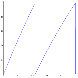
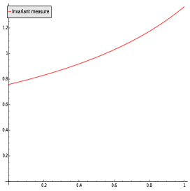
Figure 1. The map $T$ in (4.1) to the left, and its approximated invariant density to the right.

4.1. Rigorous projections on the Ulam basis

To compute the diffusion coefficient rigorously we have to compute rigorously the projection of an observable on the Ulam basis, i.e., given an observable $\phi$ in $BV$, and the projection $\Pi_{\varepsilon}$ we need to compute rigorously the coefficients $\{v_{0},\ldots,v_{n}\}$ such that

$$\Pi_{\varepsilon}\phi=\sum_{i=0}^{n-1}v_{i}\cdot\frac{\chi_{I_{i}}}{m(I_{i})},$$

where

$$v_{i}=\int_{I_{i}}\phi\,dm.$$

To do so, we will use rigorous integration through interval arithmetics, as explained in the book [35].

Once an observable is projected on the Ulam basis, many operations involved in the computation of the diffusion coefficient become componentwise operations on vectors; we explain this point in more details.

The first operation is the integral with respect to Lebesgue measure of an observable projected on the Ulam basis. This is given by the following formula:

$$\int_{0}^{1}\Pi_{\varepsilon}\phi\,dm=\int_{0}^{1}\sum_{i=0}^{n}v_{i}\frac{\chi_{I_{i}}}{m(I_{i})}\,dm=\sum_{i}v_{i}.$$

Suppose now we have computed an approximation $h_{\varepsilon}$ of the invariant density with respect to the partition, i.e., $\int_{0}^{1}h_{\varepsilon}dx=1$. In the following we will denote its coefficients on the Ulam basis by $\{w_{0},\ldots w_{n}\}$. Note that the $i$-th component, $w_{i}$, is the measure of $I_{i}$ with respect to the measure $h_{\varepsilon}dm$.

The second operation we are interested in is the pointwise product of functions and the relation of the projection $\Pi_{\varepsilon}$ with this operation. We claim that:

$$\Pi_{\varepsilon}(\phi\cdot h_{\varepsilon})(x)=\Pi_{\varepsilon}\phi(x)\cdot h_{\varepsilon}(x).$$

We will prove this by expressing the components of $\Pi_{\varepsilon}(\phi\cdot h_{\varepsilon})$ as a function of the components $\{w_{0},\ldots,w_{n}\}$ of $h_{\varepsilon}$ and the components $\{v_{0},\ldots,v_{n}\}$ of $\Pi_{\varepsilon}\phi$. We claim that

$$\Pi_{\varepsilon}(\phi\cdot h_{\varepsilon})_{i}=\frac{v_{i}\cdot w_{i}}{m(I_{i})}.$$

First of all recalling that $\chi_{I_{i}}^{2}=\chi_{I_{i}}$ and that $\chi_{I_{i}}\cdot\chi_{I_{j}}=0$ for $i\neq j$ we have:

$$\sum_{i}\frac{v_{i}\cdot w_{i}}{m(I_{i})}\cdot\frac{\chi_{I_{i}}(x)}{m(I_{i})} =\sum_{i}v_{i}\cdot\frac{\chi_{I_{i}}(x)}{m(I_{i})}\sum_{i}w_{j}\cdot\frac{\chi_{I_{j}}(x)}{m(I_{j})}=(\Pi_{\varepsilon}\phi)(x)\cdot h_{\varepsilon}(x).$$

On the right hand side, since $h_{\varepsilon}$ is constant on each $I_{i}$ and equal to $w_{i}$, we have:

$$(\Pi_{\varepsilon}(\phi h_{\varepsilon}))_{i}=\int_{I_{i}}h_{\varepsilon}\phi\,dm=\int_{I_{i}}w_{i}\cdot\frac{\chi_{I_{i}}}{m(I_{i})}\phi\,dm=\frac{w_{i}}{m(I_{i})}\cdot\int_{I_{i}}\phi\,dm=\frac{w_{i}\cdot v_{i}}{m(I_{i})}.$$

These identities simplify the computations when dealing with the Ulam basis. It is worth noting that these identities imply that:

$$\int_{0}^{1}\phi\cdot h_{\varepsilon}dm=\sum_{i}\frac{v_{i}\cdot w_{i}}{m(I_{i})}.$$

Moreover, it is worth observing that, if $P_{\varepsilon}$ is the Ulam approximation and $\phi$ is an observable:

$$P_{\varepsilon}(\phi\cdot h_{\varepsilon})=\Pi_{\varepsilon}P\Pi_{\varepsilon}(\phi\cdot h_{\varepsilon})=\Pi_{\varepsilon}P\Pi_{\varepsilon}\Pi_{\varepsilon}(\phi\cdot h_{\varepsilon})=P_{\varepsilon}(\Pi_{\varepsilon}\phi\cdot h_{\varepsilon}).$$

4.2. Item (1) in Algorithm 3.1

In this step, we find $l^{\ast}$ such that item (1) of Algorithm 3.1 is satisfied. In particular we want to find $l^{\ast}$ such that

$$4||\psi||_{\infty}\sum_{i=l^{\ast}}^{+\infty}||P^{i}((\hat{\psi}\cdot h))||_{1}\leq\frac{\tau}{256}.$$

As explained in Remark 3.3, instead of verifying item (1) to be smaller than $\frac{\tau}{2}$, we verify that it is smaller than $\frac{\tau}{256}$. This will give us more room in verifying item (2) so that the sum of the errors from both items is smaller than $\tau$. Since the system satisfies (A2), there exist $0<\rho_{\ast}<1$, and $C_{\ast}>0$ such that for any $g\in BV_{0}$, and any $k\in\mathbb{N}$,

(4.2) $$\|P^{k}g\|_{1}\leq C_{\ast}\rho_{\ast}^{k}\|g\|_{BV}.$$

We want to find a $0<\rho_{\ast}<1$ and a $C_{\ast}>0$ so that (4.2) is satisfied.

Once these two numbers are computed, we can easily find $l_{\ast}$ (see (3.5)) so that item (1) is satisfied. To compute $\rho^{\ast}$ and $C_{\ast}$ we follow [16] whose main idea is to build a system of iterated inequalities governed by a positive matrix $\mathcal{M}$ such that:

(4.3) $$\left(\!\begin{array}[]{c}\|\mathnormal{P}^{in_{1}}g\|_{BV}\\ \|\mathnormal{P}^{in_{1}}g\|_{L^{1}}\end{array}\!\right)\preceq\mathcal{M}^{i}\left(\!\begin{array}[]{c}\|\mathnormal{g}\|_{BV}\\ \|\mathnormal{g}\|_{L^{1}}\end{array}\!\right),$$

where $\preceq$ means component-wise inequalities, e.g. for vectors $\overrightarrow{x}=(x_{1},x_{2})$ and $\overrightarrow{y}=(y_{1},y_{2})$, if $\overrightarrow{x}\preceq\overrightarrow{y}$, then, $x_{1}\leq y_{1}$ and $x_{2}\leq y_{2}$.

By using Lemma 2.2 and Appendix A, we get that, if $||P^{n}_{\varepsilon}|_{BV_{0}}||_{1}\leq\alpha_{2}$, the following inequalities are satisfied:

(4.4) $$\begin{cases}\|P^{n_{1}}f\|_{BV}\leq\alpha^{n_{1}}\|f\|_{BV}+(\frac{B_{0}}{1-\alpha})\|f\|_{1}\\ \|P^{n_{1}}f\|_{1}\leq\alpha_{2}\|f\|_{1}+\varepsilon M((\frac{1+\alpha}{1-\alpha})\|f\|_{BV}+B_{0}{n_{1}}(1+\alpha+M)\|f\|_{1}.\end{cases}$$

Using the inequalities above we have that:

$$\mathcal{M}=\begin{pmatrix}\alpha^{n_{1}}&B\\ \varepsilon M(\frac{1+\alpha}{1-\alpha})&\varepsilon MB_{0}{n_{1}}(1+\alpha+M)+\alpha_{2}\end{pmatrix}.$$

Following the ideas of [16] we have that

(4.5) $$\|P^{kn_{1}}g\|_{1}\leq\frac{1}{b}\rho_{*}^{k}\|g\|_{BV},$$

where $\rho_{*}$ is the dominant eigenvalue of $\mathcal{M}$ and $(a,b)$ is the corresponding left eigenvector.

Thus, our main task now is to identify all the entries of the above matrix. The first one is $M$, a bound on the $L^{1}$ norm of the iterates of $P$ and $P_{\varepsilon}$; by definition, we have that $||P^{n}||\leq 1$ and $||P_{\varepsilon}||_{1}\leq 1$, therefore $M=1$. The two constants $\alpha_{2}$ and $n_{1}$ in $\mathcal{M}$ are two constants that give us an estimate of the speed at which $P_{\varepsilon}$ contracts the space $BV_{0}$. Let $P_{\varepsilon}$ be the discretized Ulam operator and fix $\alpha_{2}<1$; we want to find and $n_{1}\geq 0$ such that $\forall v\in BV_{0}$

(4.6) $$\|P_{\varepsilon}^{n_{1}}v\|_{1}\leq\alpha_{2}\|v\|_{1}$$

with $\alpha_{2}<1$. We follow the idea of [15] and use the computer to estimate $n_{1}$ with a rigorous computation; we refer to their paper for the algorithm used to certify $n_{1}$ and the corresponding numerical estimates and methods. Consequently, (4.3) is satisfied with $n_{1}=28$ , $\alpha\leq 0.66666667$, $B\leq 1.444444445$, $\varepsilon=1/16384$, $M=1$, $\alpha_{2}=1/64$; i.e.,

$$\mathcal{M}=\begin{pmatrix}1.18\cdot 10^{-5}&4.3333334\\ 0.000306&0.022208\end{pmatrix}.$$

Thus, $\rho_{*}=0.05$ and the eigenvector $(a,b)$ associated to the eigenvalue $\rho_{*}$ is given by $a\in[0.006,0.007]$, $b\in[0.993,0.994]$.

Thus, by (4.5), we obtain

$$\|P^{28k}g\|_{L^{1}}\leq(1.007)\times 0.05^{k}\|g\|_{BV}$$

Consequently we can compute $l_{*}\geq 112$.

Remark 4.1.

Using equation (4.5) and supposing $l_{\ast}=k\cdot n_{1}$ we see that, for any $\psi$ in $BV_{0}$:

$$\sum_{i=l_{\ast}}^{+\infty}||P^{i}(\psi)||_{1}\leq||\psi||_{BV}\frac{1}{b}\cdot n_{1}\sum_{i=k}^{+\infty}\rho_{\ast}^{i}\leq||\psi||_{BV}\frac{1}{b}n_{1}\frac{\rho_{\ast}^{k}}{1-\rho_{\ast}}.$$

4.3. Item (2) of Algorithm 3.1

From now on $l_{*}$ is fixed and it is equal to $112$. So far, we executed the first loop of the Algorithm 3.1; i.e.,

$$4\|\psi\|_{\infty}\sum_{i=112}^{\infty}\|P^{i}(\hat{\psi})\|_{1}\leq\frac{\tau}{256}.$$

Remark 4.2.

Note in our computation above we have obtained $l_{*}$ such that

$$4||\psi||_{\infty}\sum_{i=l^{\ast}}^{+\infty}||P^{i}((\hat{\psi}\cdot h))||_{1}\leq\frac{0.01}{256}\leq\frac{\tau}{256}.$$

4.4. Item (3) of Algorithm 3.1

In this step, we have to find $\varepsilon_{*}$, a mesh size of the Ulam discretization, such that

(4.7) $$\begin{split}&(16(l_{*}-1)+8)\cdot\|\psi\|_{\infty}^{2}\cdot\|h_{\varepsilon_{*}}-h\|_{1}\\ &+4\|\psi\|_{\infty}\sum_{i=1}^{l_{*}-1}\sum_{j=0}^{i-1}\bigg{(}2\|\psi\|_{\infty}(B_{j}+1+\frac{\alpha^{j}B_{0}}{1-\alpha})+\frac{\alpha^{j}(B_{0}+1-\alpha)}{1-\alpha}V\psi\bigg{)}|||P_{\varepsilon_{*}}-P|||\\ &\leq\frac{255}{256}\tau.\end{split}$$

To bound this term we need a rigorous approximation of the $T$-invariant density $h$, in the $L^{1}$-norm; we follow the ideas (and refer to the algorithm) of [15]. Set:

(4.8) $$\kappa:=4\|\psi\|_{\infty}|||P_{\varepsilon_{\ast}}-P|||\sum_{i=1}^{l_{\ast}-1}\sum_{j=0}^{i-1}\bigg{(}2\|\psi\|_{\infty}(B_{j}+1+\frac{\alpha^{j}B_{0}}{1-\alpha})+\frac{\alpha^{j}(B_{0}+1-\alpha)}{1-\alpha}V\psi\bigg{)}.$$

The following table contains, for different mesh sizes $\varepsilon$, error bounds for the terms in equation (4.7); in particular a bound on $\kappa$ defined in (4.8):

$\varepsilon$	$2^{-12}$	$2^{-24}$	$2^{-25}$
$\|h_{\varepsilon_{\ast}}-h\|_{1}\leq$	$0.016$	$3.2\cdot 10^{-5}$	$1.7\cdot 10^{-5}$
$(16(l_{\ast}-1)+8)\cdot\|\psi\|_{\infty}^{2}\cdot\|h_{\varepsilon_{\ast}}-h\|_{1}\leq$	$28.55$	$0.0571$	$0.0304$
$\kappa\leq$	$8.08$	$0.0079$	$0.00395$.

4.5. Item (4) in Algorithm 3.1

$$|\sigma_{\varepsilon_{\ast},l_{\ast}}^{2}-\sigma^{2}|\leq 0.01/256+(0.0304+0.00395)\cdot 255/256\leq 0.0342,$$

and we compute $\sigma_{\varepsilon_{\ast},l_{\ast}}^{2}$

$$\sigma_{\varepsilon_{\ast},l_{\ast}}^{2}:=\int_{I}\hat{\psi}_{\varepsilon_{\ast}}^{2}h_{\varepsilon_{\ast}}dm+2\sum_{i=1}^{l_{\ast}-1}\int_{I}P_{\varepsilon_{\ast}}^{i}(\hat{\psi}_{\varepsilon_{\ast}}h_{\varepsilon_{\ast}})\hat{\psi}_{\varepsilon_{\ast}}dm\in[0.38,0.381].$$

Remark 4.3.

The code implementing rigorous computation of diffusion coefficients for piecewise uniformly expanding maps is avalaible at the research section of the following personal page:

http://www.im.ufrj.br/nisoli/

4.6. A non rigorous verification

We also perform a non-rigorous experiment to compute $\sigma^{2}$ in the above example. Let $\mathcal{F}_{\zeta}$ be the set of floating point numbers in $[0,1]$ with $\zeta$ binary digits.

Note that the system has high entropy, so we have to be careful in our computation and choose $\zeta$ big. Due to high expansion of the system, in few iterations the ergodic average along the simulated orbit may have little in common with the orbit of the real system. So, we have to do computations with a really high number of digits ($\zeta=1024$ binary digits).

Let $\{x_{0},\ldots,x_{n-1}\}$ be $n$ random floating points in $\mathcal{F}_{l}$; fix $k$ and for each $i=0,\ldots,n-1$ let

$$A_{k}(x_{i})=\frac{1}{k}\sum_{j=0}^{k-1}\phi(T^{j}(x_{i})).$$

Let $\mu$ be an approximation of the average of $\phi$ with respect to the invariant measure, obtained by integrating the observable using the approximation of the invariant density:

$$\mu=[0.383,0.384].$$

Now, for each point $\{x_{0},\ldots,x_{n-1}\}$ we compute the value $A_{k}(x_{0}),\ldots,A_{k}(x_{n-1})$ and from these we compute the following two estimators:

$$\tilde{\mu} =\frac{1}{n}\sum_{i=0}^{n-1}A_{k}(x_{i})$$

$$\tilde{\sigma}^{2} =\frac{1}{n}\sum_{i=0}^{n-1}\frac{(k\cdot A_{k}(x_{i})-k\mu)^{2}}{k}.$$

The estimator $\tilde{\mu}$ gives a non-rigorous estimate for the average of the observable with respect to the invariant measure, while the estimator $\tilde{\sigma}^{2}$ is an estimator for the diffusion coefficient.

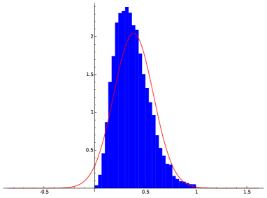
(a) $k=10$

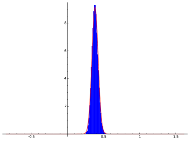
(b) $k=200$

Figure 2. Distribution of the averages $A_{k}(x_{i})$, $i=0,\ldots,19999$ for Lanford’s map.

The table below shows the outcome of the experiment with $n=20000$. In Figure 2, a histogram plot of the distribution of $A_{k}(x_{i})$ for $k=10$, $k=200$, $n=20000$. In red we have the normal distribution with average $\mu$ and variance $\sigma_{\varepsilon_{*},l_{*}}^{2}/\sqrt{k}$.

$k$	$\tilde{\mu}$	$\tilde{\sigma}^{2}$
$90$	$[0.383,0.384]$	$[0.361,0.362]$
$95$	$[0.383,0.384]$	$[0.362,0.363]$
$100$	$[0.383,0.384]$	$[0.362,0.363]$

The output of this non-rigourous experiment is in line with the output from our rigorous computation in subsection 4.5.

Appendix A Proof of equation 4.4

Lemma A.1.

$$\|(P^{n}-P^{n}_{\varepsilon})f\|_{1}\leq\varepsilon((\frac{1+\alpha}{1-\alpha})\|f\|_{BV}+B_{0}n(2+\alpha)\|f\|_{1}.$$

Proof.

$$\|\Pi_{\varepsilon}\|_{1}=\frac{\|\frac{1}{\lambda(I_{k})}\int_{I_{k}}fd\lambda\|_{1}}{\|f\|_{1}}\leq 1.$$

$$\|P^{n}\|_{1}=\|P_{\varepsilon}^{n}\|=1.$$

$$\|(P-P_{\varepsilon})f\|_{1}\leq\|\Pi_{\varepsilon}P\Pi_{\varepsilon}f-\Pi_{\varepsilon}Pf\|_{1}+\|\Pi_{\varepsilon}Pf-Pf\|_{1}=\|\Pi_{\varepsilon}P(\Pi_{\varepsilon}f-f)\|_{1}+\|\Pi_{\varepsilon}Pf-Pf\|_{1}.$$

$$\|\Pi_{\varepsilon}P(\Pi_{\varepsilon}f-f)\|_{1}\leq\|\Pi_{\varepsilon}f-f\|_{1}\leq\varepsilon V(f)\leq\varepsilon\|f\|_{BV};$$

$$\|\Pi_{\varepsilon}Pf-Pf\|_{1}\leq\varepsilon\|Pf\|_{BV}\leq\varepsilon(\alpha\|f\|_{BV}+B_{0}\|f\|_{1}).$$

$$\|(P-P_{\varepsilon})f\|_{1}\leq\varepsilon\|f\|_{BV}+\varepsilon(\alpha\|f\|_{BV}+B_{0}\|f\|_{1})\leq\varepsilon((1+\alpha)\|f\|_{BV}+B_{0}\|f\|_{1}).$$

$$\|(P^{n}-P^{n}_{\varepsilon})f\|_{1}\leq\sum_{k=1}^{n}\|P^{n-k}_{\varepsilon}(P-P_{\varepsilon})P^{k-1}f\|_{1}\leq\|(P-P_{\varepsilon})P^{k-1}f\|_{1}$$

$$\leq\varepsilon\sum_{k=1}^{n}((1+\alpha)\|P^{k-1}f\|_{BV}+B_{0}\|P^{k-1}f\|_{1})$$

$$\leq\varepsilon\sum_{k=1}^{n}((1+\alpha)(\alpha^{k-1}\|f\|_{BV}+(\frac{B_{0}}{1-\alpha})\|f\|_{1})+B_{0}\|f\|_{1})$$

$$\leq\varepsilon((\frac{1+\alpha}{1-\alpha})\|f\|_{BV}+B_{0}n(2+\alpha)\|f\|_{1}.$$

∎

References

- [1] Bahsoun, W., Rigorous numerical approximation of escape rates, Nonlinearity, 19 (2006), no. 11, 2529-2542.
- [2] Bahsoun, W., Bose, C., Invariant Densities and Escape Rates: Rigorous and Computable Approximations in The -norm. Nonlinear Analysis, 2011, vol. 74, 4481–4495.
- [3] Bahsoun, W. and Bose, C. and Duan, Y., Rigorous Pointwise approximations for invariant densities of nonuniformly expanding maps, Ergodic Theory and Dynamical Systems, 35 (2015), no. 4, 1028–1044..
- [4] Baladi, V. Positive transfer operators and decay of correlations. Advanced Series in Nonlinear Dynamics, 16. World Sci. Publ., NJ, 2000.
- [5] Bose, C., Murray, R., The exact rate of approximation in Ulam’s method. Discrete Contin. Dynam. Systems 7 (2001), no. 1, 219–235.
- [6] Boyarsky, A., Góra, P., Laws of Chaos, Invariant measures and Dynamical Systems in one dimension, Birkhäuser, (1997).
- [7] Dellnitz, M., Froyland, G., Horenkamp, C., Padberg-Gehle, K., Gupta, A. S., Seasonal variability of the subpolar gyres in the SouthernOcean: a numerical investigation based on transfer operators. Nonlinear Processes in Geophysics, 16:655-664, 2009
- [8] Dolgopyat, D., Limit theorems for partially hyperbolic systems. Trans. Amer. Math. Soc. 356 (2004), no. 4, 1637–1689.
- [9] Froyland, G., Finite approximation of Sinai-Bowen-Ruelle measures for Anosov systems in two dimensions. Random Comput. Dynam. 3 (1995), no. 4, 251–263.
- [10] Froyland, G. Using Ulam’s method to calculate entropy and other dynamical invariants. Nonlinearity 12 (1999), no. 1, 79–101.
- [11] Higham. : Accuracy and Stability of Numerical Algorithms, 2nd edition (2002) SIAM publishing, Philadela (PA), US, ISBN 0-89871-521-0.
- [12] Hofbauer, F., Keller, G. Ergodic properties of invariant measures for piecewise monotonic transformations. Math. Z. 180 (1982), no. 1, 119–40.
- [13] Holland, M., Melbourne, I. Central limit theorems and invariance principles for Lorenz attractors. J. Lond. Math. Soc. (2) 76 (2007), no. 2, 345–364.
- [14] Galatolo, S., Nisoli, I., Rigorous computation of invariant measures and fractal dimension for piecewise hyperbolic maps: 2D Lorenz like maps To appear in Ergodic Theory and Dynamical Systems doi: 10.1017/etds.2014.145
- [15] Galatolo, S., Nisoli, I., An elementary approach to rigorous approximation of invariant measures. SIAM J. Appl. Dyn. Syst. 13 (2014), no. 2, 958–985.
- [16] Galatolo, S., Nisoli, I., Saussol, S., An elementary way to rigorously estimate convergence to equilibrium and escape rates. Journal of Computational Dynamics, 2 (2015), no. 1,51–64.
- [17] Gouëzel, S. Central limit theorem and stable laws for intermittent maps. Probab. Theory Related Fields 128 (2004), no. 1, 82–122.
- [18] Jenkinson, O., Pollicott, M. Orthonormal expansions of invariant densities for expanding maps, Advances in Mathematics 192 (2005), 1–34.
- [19] Keller, G., Liverani, C. Stability of the spectrum for transfer operators. Ann. Scuola Norm. Sup. Pisa Cl. Sci. (4) 28 (1999), no. 1, 141–152.
- [20] Keller, G., Howard, P., Klages, R., Continuity properties of transport coefficients in simple maps. Nonlinearity 21 (2008), no. 8, 1719–1743.
- [21] O. E. Lanford III Informal Remarks on the Orbit Structure of Discrete Approximations to Chaotic Maps. Exp. Math. (1998), 317–324.
- [22] Lasota, A., Yorke, James A. On the existence of invariant measures for piecewise monotonic transformations. Trans. Amer. Math. Soc. 186 (1973), 481–488.
- [23] Liverani, C., Central Limit Theorem for Deterministic Systems, International Conference on Dynamical Systems, Montevideo 1995, a tribute to Ricardo Mane, Pitman Research Notes in Mathematics Series, 362, editor F.Ledrappier, J.Levovicz, S.Newhouse, (1996).
- [24] Liverani, C. Multidimensional expanding maps with singularities: a pedestrian approach. Ergod. Th. Dynam. Sys. 33 (2013), no. 1, 168–182.
- [25] Liverani, C. Rigorous numerical investigation of the statistical properties of piecewise expanding maps: A feasibility study, Nonlinearity, 14, no. 3, pp. 463–490, (2001).
- [26] Liverani C. Decay of correlations for piecewise expanding maps. J. Statist. Phys. 78 (1995), no. 3-4, 1111–1129.
- [27] Liverani, C., Saussol, B. and Vaienti, S., A probabilistic approach to intermittency, Ergodic theory Dynam. System, 19, (1999), 671-685.
- [28] Melbourne, I. and Nicol, M. Large deviations for nonuniformly hyperbolic systems. Trans. Amer. Math. Soc. 360 (2008), no. 12, 6661–6676.
- [29] Murray, R., Existence, mixing and approximation of invariant densities for expanding maps on . Nonlinear Anal. 45 (2001), no. 1, 37–72.
- [30] Murray, R., Ulam’s method for some non-unoformly expanding maps, Discrete. Contin. Dyn. Syst. 26, (2010), no. 3, 1007-1018.
- [31] Pianigiani, G., First return map and invariant measures, Israel J. Math., 35, (1980), 32-48.
- [32] Pollicott, M., Estimating variance for expanding maps. Preprint available at http://homepages.warwick.ac.uk/ masdbl/preprints.
- [33] Pomeau, Y., Manneville, P. Intermittent transition to turbulence in dissipative dynamical systems. Comm. Math. Phys. (74 (1980) 189–197.
- [34] Santitissadeekorn, N., Froyland, G., Monahan, A. Optimally coherent sets in geophysical flows: A new approach to delimiting the stratospheric polar vortex Physical Review E, 82:056311, 2010.
- [35] Tucker W. Auto-Validating Numerical Methods (Frontiers in Mathematics), Birkhäuser 2010.
- [36] Ulam S. M., A Collection of Mathematical Problems (Interscience Tracts in Pure and Applied Math. vol 8) (New York: Interscience), 1960.
- [37] Young, L-S, Recurrence times and rates of mixing, Israel J. Math., 110, (1999), 153-188.