Modeling and predicting the shape of the far-infrared to submillimeter emission in ultra-compact HII regions and cold clumps

Abstract

Context. Dust properties are very likely affected by the environment in which dust grains evolve. For instance, some analyses of cold clumps (7 K- 17 K) indicate that the aggregation process is favored in dense environments. However, studying warm (30 K-40 K) dust emission at long wavelength ($\lambda$$>$300 $\,{\rm\mu m}$) has been limited because it is difficult to combine far infrared-to-millimeter (FIR-to-mm) spectral coverage and high angular resolution for observations of warm dust grains.

Aims. Using Herschel data from 70 to 500 $\,{\rm\mu m}$, which are part of the Herschel infrared Galactic (Hi-GAL) survey combined with 1.1 mm data from the Bolocam Galactic Plane Survey (BGPS), we compared emission in two types of environments: ultra-compact HII (UCHII) regions, and cold molecular clumps (denoted as cold clumps). With this comparison we tested dust emission models in the FIR-to-mm domain that reproduce emission in the diffuse medium, in these two environments (UCHII regions and cold clumps). We also investigated their ability to predict the dust emission in our Galaxy.

Methods. We determined the emission spectra in twelve UCHII regions and twelve cold clumps, and derived the dust temperature (T) using the recent two-level system (TLS) model with three sets of parameters and the so-called T-$\beta$ (temperature-dust emissvity index) phenomenological models, with $\beta$ set to 1.5, 2 and 2.5.

Results. We tested the applicability of the TLS model in warm regions for the first time. This analysis indicates distinct trends in the dust emission between cold and warm environments that are visible through changes in the dust emissivity index. However, with the use of standard parameters, the TLS model is able to reproduce the spectral behavior observed in cold and warm regions, from the change of the dust temperature alone, whereas a T-$\beta$ model requires $\beta$ to be known.

1 Introduction

The study of the extended far-infrared (FIR) and submillimeter (submm) sky emission is a relatively young subject. This wavelength range is dominated by emission from large (15 to 100 nm) silicate-based interstellar grains (also called big grains, or BG) that dominate the total dust mass and radiate at thermal equilibrium with the surrounding radiation field. The FIR-to-submm emission is routinely used to infer total gas column density and mass of objects ranging from molecular clouds to entire external galaxies, assuming that dust faithfully traces the gas. Lacking sufficient observational data in the past century, the emission was expected to follow the so-called T-$\beta$ model, assuming an optically thin medium and a single dust temperature along the line of sight,

$$I_{\nu}(\lambda)=\epsilon(\lambda_{0})\left(\frac{\lambda}{\lambda_{0}}\right)^{-\beta}B_{\nu}(\lambda,T)N_{H}=Q_{abs}(\lambda)B_{\nu}(\lambda,T)N_{H},$$ (1)

with $\beta$=2. $I_{\nu}$ is the sky brigthness, $\epsilon(\lambda_{0})$ is the emissivity at the reference wavelength $\lambda_{0}$, $B_{\nu}$ is the Planck function, $T$ is the thermal dust temperature, $N_{H}$ is the hydrogen column density, and $Q_{abs}$ is the absorption efficiency. T-$\beta$ model with $\beta$=2 is the correct asymptotic behavior (toward long wavelengths) of the Lorentz model (the well-known and successful physical model for bound oscillators). The Lorentz model describes the mid-IR vibrational bands of the silicate-based interstellar grains.

Balloon (PRONAOS, Archeops) and satellite (FIRAS, WMAP) mission have measured the extended interstellar emission in various photometric FIR, submm, and mm bands. These data analyses have revealed that the FIR-to-submm emission cannot be explained by a simple extrapolation of the mid-IR emission. Based on these observations, the FIR-to-submm emission is often modeled with the T-$\beta$ model, with $\beta$ taken as a free parameter, mainly in the range 1 to 3. With a constant $\beta$ from FIR to submm and different from 2, this model became an empirical model, that can consequently hide any possible more complex dependences of the emissivity with wavelength and temperature. Two main patterns were observed:
- the observed FIR-to-submm dust emissivity ($\epsilon(\lambda)$) appears to have a more complex dependence on wavelength than described by the T-$\beta$ model: the emission spectrum becomes flatter in the submillimeter than a modified black-body emission with $\beta=2$ (Reach et al., 1995; Finkbeiner et al., 1999; Galliano et al., 2005; Paladini et al., 2007; Paradis et al., 2009, 2011). This has led to an empirical change in the optical constants of the Draine astro-silicates (Draine $\&$ Lee, 1984) for wavelengths larger than 250 $\,{\rm\mu m}$ (Li $\&$ Draine, 2001).
- the dust emissivity appears to be temperature-dependent in the way that the emissivity spectra are flatter with increasing dust temperature (Dupac et al., 2003; Désert et al., 2008; Veneziani et al., 2010). When the dust emission is modeled with the standard T-$\beta$ model, a degeneracy between T and $\beta$ parameters has been highlighted by the various methods of data fitting ($\chi^{2}$, hierarchical Bayesian, etc ). Therefore, noise can change the best-fit solution (decreasing T and increasing $\beta$, or vice versa). However, a systematic anti-correlation of $\beta$ with temperature is claimed to persist (Juvela et al., 2013). Similar variations of $\beta$ with temperature have been reported from laboratory spectroscopic experiments on amorphous dust analogs (Mennella et al., 1998; Boudet et al., 2005; Coupeaud et al., 2011).

These preliminary results have been confirmed using Herschel photometric data (Paradis et al., 2012, 2010) as part of the Hi-GAL survey, an Herschel open time key-project (PI S. Molinari) that mapped the entire Galactic plane (GP) of our Galaxy (Molinari et al., 2010a, b). In the Herschel wavelength range, dust emissivity spectral variations are often identified with a 500 $\,{\rm\mu m}$ emission excess (Gordon et al., 2010; Galliano et al., 2011; Paradis et al., 2012). In the Large Magellanic Cloud, this excess has been shown to correlate with temperature and to anti-correlate with brightness (Galliano et al., 2011). A similar behavior is found along the GP using Hi-GAL photometric data where a significant 500 $\,{\rm\mu m}$ excess is observed toward the peripheral regions of the GP (35$\degr$ $<$ l $<$ 70$\degr$), and can reach up to 16-20$\%$ of the emissivity (see Paradis et al., 2012, Fig. 1, panel A). The excess is often highest ($>$25$\%$) toward HII regions, but it does not appear to be systematic. However, the Herschel spectral coverage is limited to 500 $\,{\rm\mu m}$.

Dust emission and dust processes occurring in warm/hot environments such as ultra-compact HII (UCHII) regions are poorly known in the FIR-to-submm wavelength range. These regions are some of the most luminous objects in the Galaxy at FIR wavelengths, with dust temperatures of up to 80 K, and are ideal targets to search for warm/hot dust emission. HII regions correspond to photoionized regions surrounding O and B stars. UCHII regions are small (linear size smaller than 0.1 pc) and dense (electronic density n_e $>$ 10⁴ cm^-3), with newly formed O and B stars, before the ionized gas extends to become compact HII regions. They have been identified using the IRAS Point Source Catalog (PSC), based on the [25-12] and [60-12] colors (Wood $\&$ Churchwell, 1989a). UCHII regions have various properties (size, brightness temperature) and morphologies (cometary, spherical, core-halo, arc-like, shell, or more complex, see Peeters et al., 2002), that are significantly different from the standard Stromgren sphere model (Wood $\&$ Churchwell, 1989b) depending on the complex interaction of hot stars and their natal molecular cloud. The different morphologies of the UCHII regions come from the ambient medium surrounding the star, but also from the strong stellar winds of the O and B stars, which create a cavity in the ionized gas, or from the motion of the star through the cold molecular gas. All these conditions might affect dust properties inside the UCHII regions. Grain destruction/fracturing might take place in UCHII regions. In addition, the radiation field might modify the grain surface, which in turn might change the dust emissivity.

Table 1: Galactic coordinates (in degree) of the selected UCHII regions and cold clumps.

Regions	GLON	GLAT
IRAS 17279-3350	354.204	-0.036
IRAS 17455-2800	1.126	-0.109
IRAS 17577-2320	6.554	-0.098
IRAS 18032-2032	9.620	0.197
IRAS 18116-1646	13.873	0.282
IRAS 18317-0757	23.954	0.150
IRAS 18434-0242	29.955	-0.014
IRAS 18469-0132	31.395	-0.255
IRAS 18479-0005	32.795	0.192
IRAS 18502+0051	33.914	0.109
IRAS 19442+2427	60.885	-0.129
IRAS 19446+2505	61.477	0.091
Cold clump 1	17.923	-0.006
Cold clump 2	17.964	0.079
Cold clump 3	18.314	0.035
Cold clump 4	18.104	0.379
Cold clump 5	18.349	-0.273
Cold clump 6	18.411	-0.291
Cold clump 7	18.572	-0.431
Cold clump 8	18.559	-0.153
Cold clump 9	30.006	-0.270
Cold clump 10	41.715	0.035
Cold clump 11	42.874	-0.180
Cold clump 12	52.342	0.324

In the opposite temperature regime, cold clumps, which are associated with molecular clouds, evidence dust emitting at temperatures between $\sim$7 K and $\sim$17 K. Analyses of cold cores allow us to study the initial phases of star formation, that is the pre-stellar core fragmentation. In the past (before the Planck and Herschel observations), these objects were poorly detected in surveys covering wavelengths below 200 $\,{\rm\mu m}$ because of their low temperatures and weak emission. Some of them were already studied in the submm and mm domain with ground-based facilities, however. Recently, $\approx$10000 cold clumps have been cataloged using Planck data (Planck Collaboration, 2011), and some of them were observed with Herschel in specific programs. Their emission spectra show high dust emissivity index, sometimes as high as 3.5. This observed behavior might result from grain coagulation in dense and cold environments (Stepnik et al., 2003; Paradis et al., 2009; Kohler et al., 2011, 2012).

Althgouh FIR-to-mm emission is commonly modeled with a modified black body, an alternative model has been developped by Mény et al. (2007) and is referred to as the two-level system (TLS) model in the following. It is a physical model for silicate BG emission in the FIR-to-mm range, derived from solid-state modeling of general optical properties of the dielectric amorphous state. This model qualitatively agrees with laboratory experiments on amorphous silicates, and is coherent with some observational facts, such as the flattening of the emission at long wavelengths. It is also compatible with some observations in the amplitude of this flattening in the Galactic plane observed with Herschel data (Paradis et al., 2012). Without excluding other effects such as the temperature distributions along the line of sight, grain aggregations, and carbon layers on silicate-based grains, it is important to interpret the observations in terms of emission of dielectric grains (silicate maybe mixed with ice) that radiates at a single temperature along the line of sight. The observations can be modeled with the four free parameters of the TLS model (Paradis et al., 2011), allowing us to reproduce the Galactic diffuse medium (denoted in the following as diffuse parameters), Galactic compact sources (denoted as compact source parameters), and both environments (denoted as standard parameters). A full understanding of the observed dust emission would require a detailed analysis including radiative transfer, a distribution of grain sizes, a description of the morphology (aggregation, ice mantles, etc.) of the grains, and the true IR, FIR, and mm properties of the various materials that are present in the grain distribution (various silicates, ices and carbon types, with some control on their degree of amorphisation, hydrogenation, etc.). Some tests on temperature mixing along the line of sight in the inner Galactic plane have been performed in Paradis et al. (2012). The authors showed that the changes in the observed emissivity spectra with dust temperature cannot be accounted for by a line-of-sight effect alone, but might instead result from intrinsic variations in the dust properties that depend on the environment.

Regions	$F_{70}$	$F_{160}$	$F_{250}$	$F_{350}$	$F_{500}$	$F_{1100}$
IRAS 17279-3350 (1)	245.09$\pm$32.74	305.20$\pm$37.85	154.46$\pm$19.33	81.16$\pm$12.12	27.09$\pm$6.23	0.89$\pm$1.22
IRAS 17279-3350 (2)	19.24$\pm$7.47	16.65$\pm$6.25	8.31$\pm$3.65	2.72$\pm$1.11	0.78$\pm$0.46	0.06$\pm$ 0.03
IRAS 17455-2800 (1)	921.41$\pm$117.10	889.23$\pm$98.62	362.84$\pm$40.15	153.04$\pm$21.80	48.41$\pm$10.21	3.43$\pm$2.23
IRAS 17455-2800 (2)	31.59$\pm$16.34	35.18$\pm$15.29	26.16$\pm$9.20	12.93$\pm$4.96	4.30$\pm$1.72	0.12$\pm$0.07
IRAS 17577-2320 (1)	615.98$\pm$68.52	408.93$\pm$49.17	184.77$\pm$22.82	86.23$\pm$13.36	29.58$\pm$7.42	1.91$\pm$1.81
IRAS 17577-2320 (2)	23.21$\pm$7.66	21.64$\pm$7.89	12.38$\pm$3.86	4.58$\pm$1.53	1.91$\pm$0.59	0.11$\pm$0.05
IRAS 18032-2032 (1)	2469.66$\pm$252.86	2014.03$\pm$207.58	626.05$\pm$52.85	300.14$\pm$28.93	118.61$\pm$14.65	5.97$\pm$2.95
IRAS 18032-2032 (2)	39.31$\pm$29.51	42.27$\pm$16.37	22.11$\pm$10.21	8.26$\pm$4.07	2.44$\pm$0.82	0.11$\pm$0.04
IRAS 18116-1646 (1)	1599.22$\pm$166.58	1096.38$\pm$116.61	426.07$\pm$39.01	180.55$\pm$20.24	61.16$\pm$9.92	3.50$\pm$2.27
IRAS 18116-1646 (2)	45.06$\pm$29.29	37.45$\pm$12.57	16.82$\pm$5.32	5.93$\pm$1.70	1.69$\pm$0.65	0.10$\pm$0.04
IRAS 18317-0757 (1)	1378.92$\pm$144.14	759.41$\pm$82.87	225.24$\pm$26.13	84.00$\pm$14.14	25.89$\pm$7.51	1.77$\pm$1.78
IRAS 18317-0757 (2)	30.07$\pm$13.07	25.80$\pm$10.02	16.98$\pm$6.62	6.99$\pm$ 2.72	2.39$\pm$1.01	0.12$\pm$0.05
IRAS 18434-0242 (1)	3037.49$\pm$309.69	1801.52$\pm$187.72	367.84$\pm$37.81	229.12$\pm$24.56	83.98$\pm$12.58	3.59$\pm$2.58
IRAS 18434-0242 (2)	32.61$\pm$35.43	57.02$\pm$27.25	30.15$\pm$10.95	9.92$\pm$3.74	3.96$\pm$1.60	0.24$\pm$0.10
IRAS 18469-0132 (1)	720.85$\pm$78.44	646.83$\pm$70.46	311.22$\pm$28.98	148.69$\pm$16.71	53.52$\pm$8.52	2.28$\pm$1.72
IRAS 18469-0132 (2)	18.81$\pm$11.17	14.62$\pm$9.55	4.69$\pm$2.89	2.07$\pm$1.06	0.54$\pm$0.28	0.05$\pm$0.03
IRAS 18479-0005 (1)	2361.72$\pm$241.57	1581.69$\pm$163.89	495.22$\pm$42.90	282.81$\pm$26.81	92.69$\pm$12.09	5.82$\pm$2.79
IRAS 18479-0005 (2)	17.84$\pm$9.50	22.40$\pm$7.15	12.66$\pm$5.46	4.13$\pm$1.66	1.18$\pm$0.55	0.06$\pm$0.03
IRAS 18502+0051 (1)	1096.06$\pm$115.00	1076.50$\pm$113.54	472.44$\pm$41.11	235.61$\pm$23.78	80.35$\pm$11.35	2.86$\pm$2.11
IRAS 18502+0051 (2)	9.97$\pm$5.38	19.59$\pm$ 6.63	11.22$\pm$4.75	5.32$\pm$2.03	1.66$\pm$0.65	0.11$\pm$0.04
IRAS 19442+2427 (1)	1526.10$\pm$158.99	874.65$\pm$95.40	434.83$\pm$39.89	190.44$\pm$21.63	72.86$\pm$11.18	3.96$\pm$2.52
IRAS 19442+2427 (2)	38.06$\pm$14.83	47.92$\pm$18.29	19.69$\pm$7.66	8.57$\pm$3.61	2.34$\pm$ 0.95	0.15$\pm$0.08
IRAS 19446+2505 (1)	3851.74$\pm$392.29	1716.05$\pm$179.22	553.55$\pm$50.20	236.73$\pm$24.90	79.65$\pm$11.87	5.51$\pm$2.96
IRAS 19446+2505 (2)	134.00$\pm$79.70	70.81$\pm$35.01	25.71$\pm$10.49	8.00$\pm$3.13	2.87$\pm$0.77	0.17$\pm$0.08
Cold clump 1 (1)	7.73$\pm$2.95	13.42$\pm$4.30	10.40$\pm$3.58	4.65$\pm$2.33	2.18$\pm$1.53	0.14$\pm$0.37
Cold clump 1 (2)	0.31$\pm$0.15	0.98$\pm$0.45	0.83$\pm$0.34	0.47$\pm$0.20	0.21$\pm$0.10	0.02$\pm$0.01
Cold clump 2 (1)	79.94$\pm$12.23	107.14$\pm$15.76	68.61$\pm$10.87	31.30$\pm$6.94	13.17$\pm$4.37	0.81$\pm$1.01
Cold clump 2 (2)	0.37$\pm$0.31	1.47$\pm$0.77	1.55$\pm$0.63	0.73$\pm$0.28	0.34$\pm$0.14	0.02$\pm$0.01
Cold clump 3 (1)	-	8.89$\pm$5.52	8.16$\pm$4.70	4.64$\pm$3.19	1.82$\pm$2.08	0.09$\pm$0.20
Cold clump 3 (2)	-	1.96$\pm$0.34	1.64$\pm$0.40	0.83$\pm$0.23	0.36$\pm$0.11	0.01$\pm$0.01
Cold clump 4 (1)	5.17$\pm$2.60	9.94$\pm$3.41	11.35$\pm$3.69	7.10$\pm$2.98	3.57$\pm$1.96	0.21$\pm$0.46
Cold clump 4 (2)	0.20$\pm$0.08	1.28$\pm$0.24	1.30$\pm$0.33	0.79$\pm$0.31	0.27$\pm$0.12	0.02$\pm$0.01
Cold clump 5 (1)	4.19$\pm$3.66	19.28$\pm$8.77	25.30$\pm$9.07	17.09$\pm$6.69	7.68$\pm$4.30	0.39$\pm$0.84
Cold clump 5 (2)	0.50$\pm$0.11	2.79$\pm$1.30	3.45$\pm$1.52	2.00$\pm$0.90	0.88$\pm$0.39	0.04$\pm$0.02
Cold clump 6 (1)	-	5.57$\pm$4.65	16.25$\pm$6.76	14.30$\pm$5.54	7.50$\pm$3.78	0.21$\pm$0.63
Cold clump 6 (2)	-	1.18$\pm$0.49	1.77$\pm$0.85	1.01$\pm$0.66	0.46$\pm$0.32	0.03$\pm$0.02
Cold clump 7 (1)	4.49$\pm$2.59	4.65$\pm$2.95	4.53$\pm$2.40	4.71$\pm$2.46	2.17$\pm$1.55	0.11$\pm$0.33
Cold clump 7 (2)	0.15$\pm$0.35	2.72$\pm$0.55	2.06$\pm$0.30	0.96$\pm$0.28	0.39$\pm$0.11	0.02$\pm$0.01
Cold clump 8 (1)	-	2.48$\pm$5.75	9.00$\pm$6.41	6.62$\pm$4.45	3.12$\pm$2.66	0.13$\pm$0.61
Cold clump 8 (2)	-	1.80$\pm$0.36	2.22$\pm$0.56	1.33$\pm$0.32	0.58$\pm$0.15	0.03$\pm$0.01
Cold clump 9 (1)	104.97$\pm$14.96	189.10$\pm$25.65	139.88$\pm$17.64	74.53$\pm$11.28	31.25$\pm$6.40	1.65$\pm$1.33
Cold clump 9 (2)	0.64$\pm$0.72	6.68$\pm$2.66	6.23$\pm$2.17	3.59$\pm$1.26	1.82$\pm$0.56	0.07$\pm$0.03
Cold clump 10 (1)	2.71$\pm$1.86	10.80$\pm$3.74	8.25$\pm$3.14	3.16$\pm$1.87	1.45$\pm$1.22	0.15$\pm$0.39
Cold clump 10 (2)	0.88$\pm$0.22	2.39$\pm$0.42	1.63$\pm$0.30	0.80$\pm$0.14	0.31$\pm$0.06	0.02$\pm$0.01
Cold clump 11 (1)	0.66$\pm$0.70	3.61$\pm$3.59	4.14$\pm$4.67	3.44$\pm$3.15	1.56$\pm$1.91	0.08$\pm$0.38
Cold clump 11 (2)	-	0.75$\pm$0.21	0.97$\pm$0.39	0.42$\pm$0.16	0.20$\pm$0.09	0.01$\pm$0.01
Cold clump 12 (1)	7.57$\pm$2.86	21.31$\pm$5.20	21.78$\pm$5.13	13.39$\pm$3.93	7.19$\pm$2.76	0.30$\pm$0.55
Cold clump 12 (2)	0.02$\pm$0.04	0.65$\pm$0.28	0.95$\pm$0.37	0.63$\pm$0.27	0.28$\pm$0.11	0.02$\pm$0.01

Table 2: Fluxes (in Jy) computed in the central and surrounding part of the regions, denoted as (1) and (2).

Most studies in the FIR-to-mm domain require a realistic determination of dust temperature and dust column density over large parts of the sky. This is of primary importance for predicting the emission intensity at any other FIR-to-mm wavelengths, for determining masses, for removing some Galactic foreground components from cosmological signals (such as cosmic microwave background), which requires a very accurate extrapolation in frequency, or for determining variations in the general dust emission properties in various environments. Therefore, understanding variations in dust emissivity is crucial. The aim of this work is to compare the shape of the dust emission in different environments to investigate wheter distinct properties can be distinguished, and if so, to be able to accurately reproduce the shape of dust emission spectra in connection with the environment. However, we also wish to be able to easily predict dust emission in any regions of our Galaxy, even when the characteristics of the region, that is types of the environmment (diffuse, cold, warm), for instance, are unknown. We compare the ability of the TLS model with the three sets of parameters (diffuse, compact sources, standard), and a T-$\beta$ model with three fixed values of $\beta$ (1.5, 2, and 2.5) to fit the BG emission in warm and cold regions of the Galactic interstellar medium.

Table 3: Best-fit parameters of the TLS model derived for different environments.

Environment$/$parameters	$l_{c}$ (nm)	$A$	$c_{\Delta}$	reduced $\chi^{2}$
Galactic diffuse∗:
Diffuse parameters	23.05 $\pm$ 22.70	9.38 $\pm$ 1.38	242 $\pm$ 123	1.95
Galactic compact sources∗:
Compact source parameters	5.11 $\pm$ 0.09	3.86 $\pm$ 0.13	1333 $\pm$ 68	1.45
Galactic diffuse and compact sources∗:
Standard parameters	13.40 $\pm$ 1.49	5.81 $\pm$ 0.09	475 $\pm$ 20	2.53
UCHII regions†:
Diffuse parameters	23.05 $\pm$ 22.70	9.38 $\pm$ 1.38	242 $\pm$ 123	1.27
Galactic compact sources	5.11 $\pm$ 0.09	3.86 $\pm$ 0.13	1333 $\pm$ 68	2.09
Standard parameters	13.40 $\pm$ 1.49	5.81 $\pm$ 0.09	475 $\pm$ 20	1.28

^∗ Paradis et al. (2011).
^† This work.

The main goal of this work is to investigate the potentially distinct dust properties depending on the environment and to be able to predict the FIR-to-mm emission in cold and warm regions. In this study, we combine Bolocam with Herschel data to extend the spectral coverage to mm wavelengths (1.1 mm), which is important to detect any changes in the shape of the emission spectrum. Data from the Midcourse Space Experiment (MSX) in band E (21.3 $\,{\rm\mu m}$) and Spitzer data at 24 $\,{\rm\mu m}$ are also presented, but were not included in the modeling. In sect. 2 we briefly summarize surveys, in Sect. 3, we explain the selection of targets in the two specific environments (UCHII regions and cold clumps). We describe the method (including dust emission extraction and modeling) in Sect. 4. Discussions and conclusions are provided in Sect. 5 and 6.

2 Data

2.1 Hi-GAL survey

The Hi-GAL survey covers the entire Galactic plane (-1$\degr$ $<$b $<$+1$\degr$) at five wavelengths (70, 160, 250, 350 and 500 $\,{\rm\mu m}$), with an angular resolution going from 6^′′ to 37^′′. The data was processed with the software ROMAGAL (Traficante et al., 2011). The PACS and SPIRE absolute zero level were calibrated by applying gains and offsets derived from the comparison with the Planck-High Frequency Instrument and IRIS (Improved Reprocessing of the IRAS Survey, see Miville-Deschênes $\&$ Lagache, 2005) data (see Bernard et al., 2010; Paradis et al., 2012).

2.2 BGPS survey

With an angular resolution of 33^′′, the Bolocam Galactic Plane Survey (BGPS, Aguirre et al., 2011) covers the longitude and latitude ranges -10.5$\degr$ $\leq$ l $\leq$ 90.5$\degr$ and $\mid$b$\mid$$\leq$0.5$\degr$ in a contiguous way. Extentions in latitude were performed in some regions (Cygnus X spiral arm, l=3$\degr$, 15$\degr$, 30$\degr$ and 31$\degr$). Four regions in the outer Galaxy were also observed: IC1396, a region toward the Perseus arm, W3/4/5, and Gem OB1. The total coverage area is 170 square degrees. A full description of the BGPS can be found in Aguirre et al. (2011). The data in unit of Jy/beam, were first converted into MJy/sr using Eq. 16 from Aguirre et al. (2011), which was derived from the beam surface value. We used the new version of the data (v2.0, 2013). In this version, data no longer suffer from calibration issues, that is the 1.5 factor needed by Aguirre et al. (2011) in the previous version of the data to obtain consistency with other data sets has been made redundant. However, the processing of the maps possibly attenuates the aperture flux for structures extending to 3.8^′ by 50$\%$ .

2.3 Additional data

We also analyzed near-infrared (NIR) data such as the MSX data in band E (21.3 $\,{\rm\mu m}$, with a resolution of 20^′′) and Spitzer data (24 $\,{\rm\mu m}$, with a resolution of 6^′′) as part of the MIPSGAL program (PI: S. Carey, Carey et al., 2009) for the UCHII regions, but they were not included in the modeling (see Sect. 4.2). Most of the UCHII regions we are interested in are very bright, and some pixels of the 24 $\,{\rm\mu m}$ images were saturated. These pixels were replaced using MSX band E data at a lower resolution than the original Spitzer data, which might result in underestimated flux. The corrected 24 $\,{\rm\mu m}$ images are not yet published.

All the data were convolved to a 37^′′ angular resolution to match the resolution of the Herschel 500 $\,{\rm\mu m}$ data, with a pixel size of 13.9^′′. The resolution was changed by convoluting by a Gaussian kernel with FWHM $\sigma_{k}^{2}=\sigma_{c}^{2}-\sigma_{d}^{2}$, where $\sigma_{c}$ is the common resolution, that is 37^′′, and $\sigma_{d}$ is the original resolution of the data. The SPIRE 500 $\,{\rm\mu m}$ beam profile has a plateau at $\sim 1\%$ that extends to a radial distance of 1^′. The Gaussian approximation of the beam is still valid even for the selected annulus we consider in the following (28^′′ to 56^′, see Sect. 4.1).

To avoid any zero level mismatch between Herschel, Spitzer, MSX and Bolocam data, we subtracted a background from all images. The background was computed as the median over a common area, corresponding to the 10$\%$ lowest values in the Bolocam data.

3 Two specific environments

3.1 UCHII regions

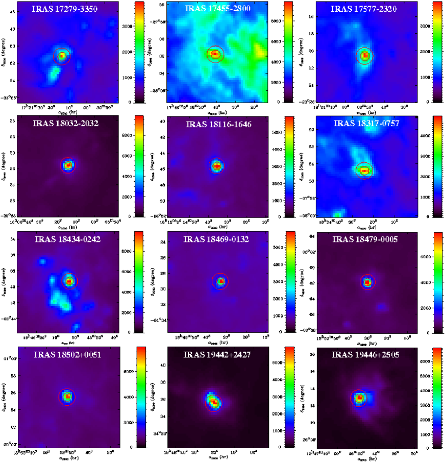
Figure 1: Herschel 350 $\,{\rm\mu m}$ images of the selected UCHII regions. The photometric apertures for which the fluxes have been computed are indicated by red circles. Central and surrounding regions are denoted (1) and (2) in the text.

The UCHII regions have been cataloged by Codella et al. (1994) using the association of HII regions and IRAS PSC. We chose twelve targets from the catalog that were observed in both the Hi-GAL and BGPS surveys and have high 100 $\,{\rm\mu m}$ IRAS fluxes ($>10^{3}$ Jy) to ensure that we studied UCHII regions that include warm dust. Because IRAS has a lower resolution than the Herschel data, the coordinates of the regions were determined from the maximum surface brightness at 160 $\,{\rm\mu m}$. Characteristics and images of the selected UCHII regions are given in Tab. 1 and Fig. 1.

3.2 Cold clumps

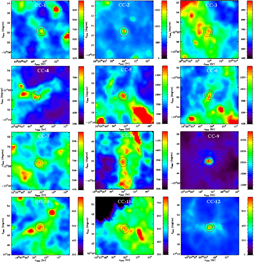
Figure 2: Herschel 350 $\,{\rm\mu m}$ images of the selected cold clump regions. The photometric apertures for which the fluxes have been computed are indicated by red circles. Central and surrounding regions are denoted (1) and (2) in the text.

We chose cold molecular clumps (previously identified from ¹³CO (observations using the BU-FCRAO Galactic Ring Survey, see Jackson et al., 2006), that were recently analyzed using a 3D - Galactic inversion on Herschel observations (Tab. 1 in Marshall et al., 2013), based on HI and ¹³CO data. In this analysis, dust temperatures in each phase of the gas have been determined for each molecular clump. We selected twelve targets that show cold dust. In the following, we refer to these regions as cold clumps, even if they do not strictly correspond to the definition adopted by the Planck collaboration. For each cloud we obtained the exact coordinates that enabled us to derive the maximum surface brigthness at 500 $\,{\rm\mu m}$ (FIR-to-submm emission peaks do not correspond to HI or ¹³CO peaks). This selection leads to coordinates different from those reported in Marshall et al. (2013). The coordinates of our cold clump selection are provided in Tab. 1. Images of the targets at 350 $\,{\rm\mu m}$ are provided in Fig. 2.

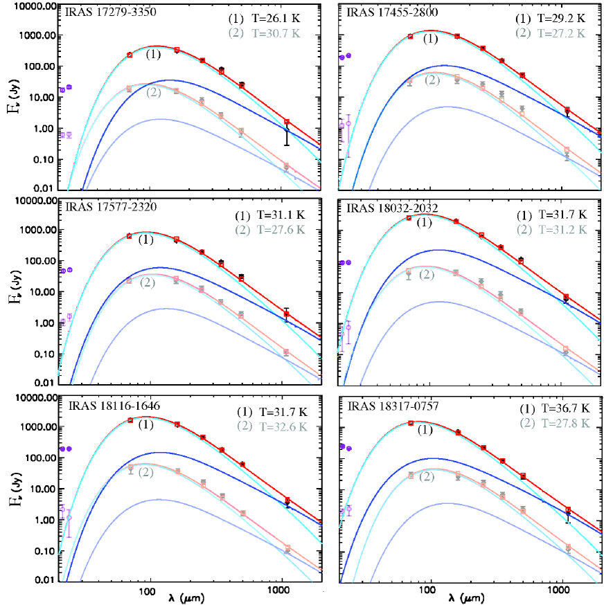
Figure 3: Herschel (70, 160, 250, 350, 500 $\,{\rm\mu m}$) - Bolocam (1.1 mm) SED (black diamonds) of UCHII regions, fitted with the TLS model using the diffuse parameters (total emission in red, DCD and TLS processes in light and dark blue). Squares represent models integrated in the band filters of each instrument, allowing direct comparisons with data (diamonds). SED corresponding to the central (1) and surrounding (2) part of the region are represented in dark and light colors. MSX data in band E (21.3 $\,{\rm\mu m}$) and Spitzer data at 24 $\,{\rm\mu m}$ are also visible in the plots, represented by the purple circles.

Figure 3: Continued.

4 Method

4.1 Aperture photometry to extract dust emission

For each UCHII region and cold clump, we extracted two spectral energy distributions (SEDs). It is more reasonable to base our analysis on two SEDs per region than on only one. Instead of determing SEDs per pixels, we constructed SEDs derived from averaging several pixels. We chose the central part of the region (denoted as -(1)- in the following) that has bright pixels (not intended to describe the core of the region), and an annulus surrounding the central part (denoted as -(2)- in the following). In this way, we expected to obtain slight changes in dust temperature farther away from the central part, to sample various temperatures. For this purpose we used the idl routine aper to compute concentric aperture photometry. We fixed the first aperture to a two-pixel radius (27.8^′′) and the surrounding annulus with an inner and outer radius of two and four pixels (between 27.8^′′ and 55.6^′′). The SED in region (1) was background subtracted from the annulus region (2). We considered as uncertainty the quadratic sum of the uncertainty deduced from the idl routine aper, which includes the dispersion on the sky background (corresponding to the root mean square of the background), and the calibration uncertainty depending on each instrument. The Hi-GAL data have been generated by the software ROMAGAL (Traficante et al., 2011), which does not remove the large-scale emission, as opposed to standard high-pass filtering. For these data, the calibration uncertainty has been estimated to be 10$\%$ for PACS (Poglitsch et al., 2010) and 7$\%$ for SPIRE (oberver’s manual v2.4). For the Bolocam data, we used a calibration uncertainty of 20$\%$, which corresponds to the comparison of the v2 version of the data with the flux from other instruments (Ginsburg et al., 2013). We note that the Bolocam data uncertainties on the output flux from the routine aper are large because of noise in the data. Adding a calibration uncertainty of 20$\%$, we obtained in some cases a total uncertainty twice (or even more) larger than the flux, which indicates a low signal-to-noise ratio. We determined the flux at each wavelength from 70 $\,{\rm\mu m}$ to 1.1 mm to obtain FIR-mm SEDs. Flux values are provided in Tab. 2. We proceeded in the same way to also deduce the 21.3 $\,{\rm\mu m}$ and 24 $\,{\rm\mu m}$ fluxes in UCHII regions. The SEDs are given in Fig. 3 and 4.

Figure 4: Herschel (70, 160, 250, 350, 500 $\,{\rm\mu m}$) - Bolocam (1.1 mm) SED (black diamonds) of cold clumps, fitted with the TLS model using the compact source parameters (total emission in red, DCD and TLS processes in light and dark blue). Squares represent models integrated in the band filters of each instrument, allowing direct comparisons with data (diamonds). 70 $\,{\rm\mu m}$ data have not been included in the fitting. SED corresponding to the central (1) and surrounding (2) part of the region are represented in dark and light colors.

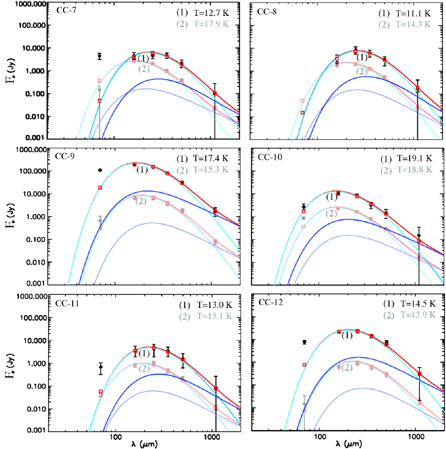
Figure 4: Continued.

4.2 Modeling

Figure 3 shows that fluxes in the NIR wavelengths are quite high, probably because of the contributon from small grains that are stochastically heated by the radiation field. Since the models used here include a single BG component, we selected a wavelength range where this component clearly dominates the overall emission. In addition, the wavelength range was restricted by the validity of both the TLS and the T-$\beta$ models. These models are only valid in the FIR-to-mm for wavelengths longer than $\sim$50 $\,{\rm\mu m}$, where the following assumptions can be made: the real part of the dielectric constant can be considered to be constant and the size of the particules can be considered to be smaller than the wavelength. Moreover, the 21 $\,{\rm\mu m}$ flux in cold clumps might be biased by the absorption resulting from the silicate bands occuring at 20 $\,{\rm\mu m}$.Therefore, the 21.3 $\,{\rm\mu m}$ and 24 $\,{\rm\mu m}$ flux were not included in the modeling.

4.2.1 T-$\beta$ model

The typical way of describing FIR emission is to use a simple modified black-body model with a fixed value of $\beta$. The common value of $\beta$ is 2. This type of model is acceptable when long wavelength constraints are not available and for regions with temperatures of about 17-20 K. However, there is no reason a unique value of $\beta$ to be applicable throughout the sky. Some authors have claimed that $\beta$ variations are only a result of calibration uncertainties on the data, temperature mixing along the line of sight (Shetty et al., 2009), or applications of the $\chi^{2}$ minimization technique. A Bayesian approach on the data modeling, however, can clearly distinguish between a real and spurious T-$\beta$ relationship (Kelly et al., 2012; Veneziani et al., 2013). Moreover, in some cases it is obvious that a modified black-body model with $\beta$=2 does not work, especially in cold regions with steep spectra ($\beta$ $\simeq 3$, see, for instance, Désert et al., 2008; Planck Collaboration, 2011), or hot regions with flat spectra ($\beta$ $\simeq 1$, see, for instance, Dupac et al., 2003; Kiuchi et al., 2004). However, this is not a systematic behavior. Some measurements of cold cores in the Taurus region between 160 and 2100 $\,{\rm\mu m}$, do not show departures of $\beta$ from $\beta=2$ (see, for instance, Schnee et al., 2010). In addition, we know that the FIR-to-mm emission varies as a function of wavelength, as observed in laboratory experiments. (Boudet et al., 2005; Coupeaud et al., 2011).

Figure 5: Herschel (70, 160, 250, 350, 500 $\,{\rm\mu m}$) - Bolocam (1.1 mm) SED (black diamonds) of IRAS 19446+2505 (1) and CC6 (2), fitted with the TLS model using the standard parameters in red, and with a T-$\beta$ model $\beta$=1.5 in purple, $\beta$=2 in green, and $\beta$=2.5 in blue. Squares represent models integrated in the band filters of each instrument, allowing direct comparisons with data (diamonds). The 70 $\,{\rm\mu m}$ Herschel data have not been included in the fits for CC6 (2). The corresponding dust temperatures for each model are given in the top right corner.

	Dust temperatures (K)
Regions	TLS				T-$\beta$
	Diff.	CS	Std.	1-$\sigma$	$\beta$=2	$\beta$=1.5	$\beta$=2.5	1-$\sigma$
IRAS 17279-3350 (1)	26.13	25.81	25.85	0.17	25.29	29.17	22.70	3.26
IRAS 17279-3350 (2)	30.72	31.27	30.73	0.31	28.68	35.29	24.71	5.34
IRAS 17455-2800 (1)	29.17	29.17	29.12	0.03	28.21	33.21	24.76	4.25
IRAS 17455-2800 (2)	27.21	26.76	26.75	0.26	24.70	31.72	20.20	5.81
IRAS 17577-2320 (1)	31.10	31.17	30.81	0.19	30.14	35.08	26.67	4.23
IRAS 17577-2320 (2)	27.57	27.67	27.30	0.19	25.78	31.56	22.26	4.70
IRAS 18032-2032 (1)	31.67	31.80	31.66	0.08	30.29	36.22	26.61	4.85
IRAS 18032-2032 (2)	31.19	33.22	31.21	1.17	27.44	36.19	22.53	6.92
IRAS 18116-1646 (1)	31.71	32.03	31.69	0.19	30.57	36.29	26.65	4.85
IRAS 18116-1646 (2)	32.63	34.25	32.68	0.92	29.13	37.68	24.59	6.65
IRAS 18317-0757 (1)	36.65	37.27	36.69	0.35	34.92	42.66	30.03	6.37
IRAS 18317-0757 (2)	27.78	28.25	27.76	0.28	25.72	32.20	21.75	5.28
IRAS 18434-0242 (1)	37.76	38.76	38.19	0.50	36.19	44.21	30.75	6.77
IRAS 18434-0242 (2)	26.20	26.14	26.13	0.04	24.48	30.62	20.69	5.01
IRAS 18469-0132 (1)	28.14	28.15	28.11	0.02	27.21	31.69	24.16	3.79
IRAS 18469-0132 (2)	33.54	34.76	33.63	0.68	30.73	38.73	26.15	6.37
IRAS 18479-0005 (1)	32.69	33.15	32.69	0.27	31.26	37.28	27.24	5.05
IRAS 18479-0005 (2)	29.26	29.75	29.24	0.29	27.03	34.20	22.72	5.80
IRAS 18502+0051 (1)	28.10	28.10	28.06	0.02	27.14	31.72	23.77	3.99
IRAS 18502+0051 (2)	24.04	23.57	23.77	0.24	22.52	27.79	18.78	4.53
IRAS 19442+2427 (1)	31.19	31.26	31.18	0.04	30.17	35.25	26.27	4.50
IRAS 19442+2427 (2)	28.74	29.15	28.71	0.25	26.96	33.23	23.17	5.08
IRAS 19446+2505 (1)	37.20	38.23	37.27	0.58	35.24	43.23	30.20	6.57
IRAS 19446+2505 (2)	37.63	41.25	38.13	1.96	33.56	43.61	27.74	8.03
Mean std. deviation	-	-	-	0.38	-	-	-	5.33
Cold clump 1 (1)	18.65	17.96	18.52	0.37	18.03	21.56	15.66	2.97
Cold clump 1 (2)	16.63	15.62	16.38	0.53	15.96	19.94	13.88	3.08
Cold clump 2 (1)	20.40	19.60	20.17	0.41	19.58	23.78	16.93	3.45
Cold clump 2 (2)	17.01	15.58	16.59	0.74	16.21	20.64	13.80	3.47
Cold clump 3 (1)	17.11	15.76	16.86	0.72	16.44	20.17	14.05	3.08
Cold clump 3 (2)	19.15	17.14	18.66	1.05	18.12	23.25	15.01	4.16
Cold clump 4 (1)	14.61	13.97	14.47	0.34	14.17	16.50	12.64	1.94
Cold clump 4 (2)	16.98	15.26	16.52	0.89	16.12	20.18	13.65	3.29
Cold clump 5 (1)	14.17	13.16	13.98	0.54	13.79	16.13	12.04	2.05
Cold clump 5 (2)	17.06	14.46	16.52	1.37	16.10	20.73	13.19	3.80
Cold clump 6 (1)	11.71	10.58	11.54	0.61	11.47	13.20	10.03	1.59
Cold clump 6 (2)	15.19	13.30	14.89	1.02	14.59	18.18	12.24	2.99
Cold clump 7 (1)	13.64	12.69	13.55	0.52	13.19	15.25	11.67	1.80
Cold clump 7 (2)	19.59	17.91	19.13	0.87	18.31	24.16	15.38	4.47
Cold clump 8 (1)	12.18	11.13	12.04	0.57	11.95	13.70	10.47	1.62
Cold clump 8 (2)	16.56	14.25	16.04	1.21	15.67	20.16	12.99	3.62
Cold clump 9 (1)	18.30	17.41	18.04	0.46	17.56	21.22	15.33	2.97
Cold clump 9 (2)	17.65	15.32	17.12	1.22	16.65	21.74	13.72	4.06
Cold clump 10 (1)	19.72	19.07	19.63	0.35	19.09	22.75	16.52	3.13
Cold clump 10 (2)	20.53	18.82	20.10	0.89	19.15	25.17	15.96	4.68
Cold clump 11 (1)	13.96	13.02	13.67	0.48	13.51	15.71	11.95	1.89
Cold clump 11 (2)	16.70	15.05	16.45	0.89	16.03	20.18	13.50	3.37
Cold clump 12 (1)	15.22	14.53	15.07	0.36	14.86	17.22	13.10	2.07
Cold clump 12 (2)	14.09	12.90	13.79	0.62	13.56	16.55	11.76	2.42
Mean std. deviation	-	-	-	0.71	-	-	-	3.00

Table 4: Dust temperatures (in K) derived from the TLS and T-$\beta$ models, using different sets of parameters (diffuse, compact sources and standard parameters) and $\beta$ values (1.5, 2 and 2.5), respectively. 1-$\sigma$ correspond to the standard deviation of dust temperature derived from the three set of TLS parameters or three $\beta$ values. The mean values of the 1-$\sigma$ columns are also given.

4.2.2 TLS model

The TLS model is the first model that takes the physical aspect of amorphous dust material into account. We do not give a full description of the TLS model here, but refer to Mény et al. (2007) for a theoretical overview of the physics of the model and to Paradis et al. (2011, 2012) for comparisons of the TLS model with astrophysical data (FIRAS/WMAP, Archeops and Herschel data). In previous analyses, we determined the best parameters that allowed us to reproduce the Galactic diffuse medium (denoted as diffuse parameters, or Diff.), Galactic compact sources (denoted as compact sources parameters, or CS) and both environments (denoted as standard parameters, or Std.). The TLS model is the combines two distinct processes: the disordered charge distribution (DCD) part at the grain scale, and the TLS part itself at the atomic scale. The first effect describes the interaction between the electromagnetic wave and acoustic oscillations in the disordered charge of the amorphous material (Vinogradov, 1960; Schlomann, 1964). This DCD process is characterized by a correlation lenght ($l_{c}$), that controls the inflection point where two asymptotic behaviors occur ($\epsilon\propto\lambda^{-2}$ and $\epsilon\propto\lambda^{-4}$). The TLS process takes the interaction of the electromagnetic wave with the simple distribution of an asymmetric double-well potential into account (Phillips, 1972, 1987; Anderson et al., 1972). This TLS process is characterized by three specific effects that are temperature-dependent, which is different from the DCD process. One of these TLS effects is represented by the parameter $c_{\Delta}$ that describes the tunneling states. The amplitude of the TLS effects with respect to the DCD process is controled by a multiplying factor denoted $A$, that is, $I_{tot}=I_{DCD}+A\sum I_{TLS}$.
In the following we therefore use the three sets of parameters (Diff., CS, Std.), fixed to some specific values of $l_{c}$, $c_{\Delta}$, and $A$ (see Tab. 3) that were derived from previous analyses (Paradis et al., 2011), when performing SED fitting with the TLS model.

Table 5: Results of the polynomial fit (see Eq. 4) for the TLS model for each environment.

Environment	$k_{0,i}$	$k_{1,i}$	$k_{2,i}$	$k_{3,i}$	$k_{4,i}$
Diffuse medium	3.33830	-5.36544e-3	1.65381e-6	1.63754e-11	-6.88816e-12
	-2.98801e-4	1.49526e-5	-1.42524e-7	1.41845e-12	6.72034e-13
	8.54787e-6	-2.17671e-7	1.49001e-9	1.03925e-11	-2.48183e-14
	-3.25327e-8	1.06390e-9	4.20971e-12	-1.37459e-13	2.39831e-16
	4.55497e-11	-1.10996e-12	-3.84120e-14	4.36257e-16	-6.77351e-19
Compact sources	3.34100	-6.57687e-3	1.67055e-5	-7.42107e-8	7.97846e-11
	-1.78243e-3	8.93472e-5	-1.09494e-6	3.82566e-9	-2.98224e-12
	4.27571e-5	-1.54310e-6	1.94520e-8	-5.15802e-11	2.51914e-14
	-2.53887e-7	1.06665e-8	-1.19930e-10	2.44969e-13	-2.12459e-17
	5.47140e-10	-2.43342e-11	2.47310e-13	-3.67727e-16	-2.21749e-19
Standard medium	3.33042	-5.49209e-3	2.14115e-6	-2.14173e-9	-7.90430e-12
	-2.84206e-4	1.12572e-5	-1.11099e-7	-7.48509e-11	9.32649e-13
	9.23806e-6	-1.28278e-7	1.17408e-9	1.19308e-11	-3.01610e-14
	-3.20750e-8	4.97171e-10	5.92135e-12	-1.52179e-13	2.83618e-16
	3.66206e-11	1.88461e-13	-4.33218e-14	4.82933e-16	-7.97139e-19

Table 6: Gaussian coefficients from Eqs. 4 and 5 for the three environments.

Environment	$a_{0}$	$a_{1}$	$a_{2}$	$a_{3}$	$a_{4}$	$a_{5}$
Diffuse medium	-0.00050	0.07585	5.36111	100.19785	13.47090	499.96309
Compact sources	-0.00126	0.14795	4.52068	91.28719	9.50025	451.84591
Standard medium	-0.00062	0.09271	5.14453	90.71464	12.36827	484.87299

4.2.3 $\chi^{2}$ minimization

We performed $\chi^{2}$ minimizations on SEDs using both models (see Tab. 7). For the T-$\beta$ model we applied three values of $\beta$ (1.5, 2, and 2.5). For the TLS model we used the three sets of parameters defined in the previous section. The three $\beta$ values of 1.5, 2, and 2.5 are not arbitrary values. At first order, a mean emissivity spectral index in the submm domain derived from the TLS model is close to 2, with the use of standard parameters in the range $\sim$17-25 K, 1.5 with diffuse parameters in the range $\sim$30-40 K, and 2.5 with CS parameters in the range $\sim$8-13 K. In that sense, the choice of these three $\beta$ values is similar to that of the submm slope derived from the TLS model. However, the slope in the FIR in the TLS model is different from the slope in the submm and mm because of the DCD process in the FIR and TLS processes in the submm and mm. This change of $\beta$ from FIR to submm and mm has been observed in various environments (see, for instance, Paradis et al., 2009; Planck Collaboration, 2014; Gordon et al., 2014) For the UCHII regions the $\chi^{2}$ minimizations was made between 70 $\,{\rm\mu m}$ and 1.1 mm, while for cold clumps the 70 $\,{\rm\mu m}$ flux was not included in the fits. For environmental temperatures higher than $\simeq$25 K, the 70 $\,{\rm\mu m}$ flux arises by more than 85$\%$ from big grains in equilibrium with the interstellar radiation field, according to the DustEM model (Compiègne et al., 2011). However, in cold environments, the 70 $\,{\rm\mu m}$ emission includes a substantial fraction of emission from small grains that constantly fluctuate in temperature after a photon absorption/emission. We pre-computed the brightness in the Herschel and Bolocam filters by applying the color correction necessary for each instrument using both models, for temperatures ranging from 5 to 50 K, sampled every 0.5 K. The $\chi^{2}$ value was computed for each value of the grid, and we chose the value of the dust temperature that minimizes the $\chi^{2}$. To allow interpolating between individual entries of the table, the best-fit temperature value ($T^{\star}$) was computed for the ten lowest values of $\chi^{2}$ as

$$T^{\star}=\frac{\sum_{i=1}^{10}T_{i}\times\frac{1}{\chi^{2}_{i}}}{\sum_{i=1}^{10}\frac{1}{\chi^{2}_{i}}}.$$ (2)

Temperatures derived from the fits are given in Tab. 4. The models were adjusted to the data by adopting the following normalization:

$$F_{model,norm}(\lambda)=\frac{F_{model}(\lambda)\times\sum_{\lambda}F_{obs}(\lambda)}{\sum_{\lambda}F_{model}(\lambda)},$$ (3)

where $F_{model}$ and $F_{model,norm}$ are the integrated flux in each band deduced from the model before and after normalization, respectively, and $F_{obs}$ is the observed flux. The sum over the fluxes is performed between 70 and 500 $\,{\rm\mu m}$ for SEDs of UCHII regions, and between 100 and 500 $\,{\rm\mu m}$ for SEDs of cold clumps. We note that the dispersion in temperature values can be significant from one model to the other and from one set of parameters to the other, but in the latter case the $\chi^{2}$ dispersion is high as well. For instance, Tab. 4 shows that the mean value of temperature dispersion is 5.33 K and 3.00 K for UCHII regions and cold clumps with T-$\beta$ models while it is of 0.38 K and 0.71 K for the TLS model. The comparison of temperatures derived from fits with the TLS model (diffuse parameters) and T-$\beta$ model ($\beta=1.5$) with similar $\chi^{2}$ illustrates the dispersion: 6.45 K for IRAS 18434-0242 (1) (37.76 K and 44.21 K for the TLS and T-$\beta$ model); $\sim$5 K for IRAS 18469-0132 (2) (33.54 K and 38.73 K) and IRAS 18032-2032 (2) (31.19 and 36.19 K). The dispersion is lower for the fitting of cold clumps (with CS parameters and $\beta$=2.5): 1.71 K for CC3 (1) (15.76 K and 14.05 K); 1.61 K for CC4 (2) (15.26 K and 13.65 K); and 1.27 K for CC5 (2) (14.46 K and 13.19 K). The results show that the choice of the model has a real and strong impact on the temperature determination. In the TLS model, the temperature determination is much less sensitive to the slope of the emissivity at long wavelengths. This is because, in agreement with laboratory data on silicates between 10 K and 100 K, the slope of the emissivity starts flattening with temperature in the submm range, while the temperature is mainly deduced from the FIR domain ($\lambda<350$ $\,{\rm\mu m}$) in the observational data. Indeed, in the framework of the TLS model, an observed dust emissivity index far from a value equal to 2 in the 100-350 $\,{\rm\mu m}$ range cannot arise from intrinsic properties of silicate grains, but only from a possible grain temperature distribution and from big grains containing carbon, for instance. On the other hand, in a T-$\beta$ model, the dust emissivity index is kept constant over the whole FIR-to-mm range and consequently in the range near the peak of emission, which is required for an accurate temperature determination. Therefore, for futures studies on optical properties variations with environment (and temperature as a consequence), the TLS model does not present the same artifact in terms of temperature determination as a T-$\beta$ model, and is in particular a better description of the FIR-to-mm emission.

5 Discussion

The different trends observed between the two types of environments were deduced from the statistics from 12 regions and the analysis of 24 SEDs (since we have two SEDs per region) for each environment. We essentially focused on the total sum of the $\chi^{2}$, and on the number of best fits (best $\chi^{2}$) depending on the model and its associated parameters (see Tab. 7). To assign the same weight to each SED we normalized the $\chi^{2}$ values (Tab. 7), allocating the value of 1 to the highest $\chi^{2}$ value derived from the TLS model for each SED. This normalization ensures that the total $\chi^{2}$ is not unaffected by a single high $\chi^{2}$ value due to a bad fit. We also normalized the $\chi^{2}$ for T-$\beta$ modeling and kept the same reference value. We have checked the consistency of the SED fitting results by allowing the flux density measurements to vary within the range permitted by their uncertainties. Although the Herschel data are internally calibrated, the zero level of the background in both PACS and SPIRE data is not. For the Hi-GAL data, a strategy was adopted to set this background level using the IRIS and Planck calibrations (see Sect. 2). For the cold clumps, in particular, the entire SED wavelength range from 160 to 500 $\,{\rm\mu m}$ was cross-calibrated using the Planck data. This allowed us to have consistent flux density uncertainties, so that the spectral shape was not affected by the above method. Moreover, the Bolocam data have large intrinsic uncertainties that are dominated by the noise (Bally et al., 2010); they do not affect the SED fits and therefore were not touched during the tests. For the UCHII region SEDs, the 70 $\,{\rm\mu m}$ measurements were cross-calibrated using a combination of IRIS and Planck calibration, therefore we experimented some more with the uncertainties. We performed two tests; one consisting of shifting the 70 $\,{\rm\mu m}$ values up according to the derived uncertainty of the IRIS 70 $\,{\rm\mu m}$, and shifting the values from 160 to 500 $\,{\rm\mu m}$ down, using the Planck uncertainties. We then perfomed the opposite case (shifting the 70 $\,{\rm\mu m}$ flux down and shifting the flux from 160 to 500 $\,{\rm\mu m}$ up. For all SEDs, the best models still correspond to those identified in Tab. 7, that is, we obtained similar results. Only the dust temperatures are affected by exploring the range allowed by the uncertainties, with variations of 1 K to 2.5 K depending on the SED fit.

We recall that temperature mixing was not taken into account in this analysis. This possible effect would affect TLS and T-$\beta$ models in the same way by inducing a flattening of the spectrum at first order. However, temperature mixing along the line of sight is expected in the inner Galactic plane. The Galactic Center, which is particularly exposed to these effects, showed steep spectra (Paradis et al., 2012), which contradicts expectations. Moreover, Paradis et al. (2009) investigated the effect of the interstellar radiation field strengh mixture (as well as grain size distribution and grain composition) in cold molecular clouds to explain the steeper emissivity spectra in the FIR than in the submm and mm. They concluded that these effects are responsible for the submm and mm SED flattening. Even if temperature mixing might have an impact on the spectral behavior of dust emission, it is unlikely that this would significantly affect the conclusions of our analysis here.

5.1 Specific dust properties in each environment

With the TLS modeling, the total number of best fits deduced from best $\chi^{2}$ indicates that compact source (CS) parameters do not give the best description of spectra in UCHII regions (best $\chi^{2}$ for only 12$\%$ of the SEDs), while diffuse and standard parameters give better solutions (52$\%$ and 36$\%$). For cold clumps, the former set of parameters (CS parameters) is satisfactory for 56$\%$ of the SEDs (against 8$\%$ and 36$\%$ for diffuse and standard parameters). These results cleary show that SEDs from UCHII regions and cold clumps are not reproduced by the same set of parameters; therefore they have different dust properties.

The results are similar for the T-$\beta$ models. Indeed, 62.5$\%$ of UCHII region SEDs are well reproduced using $\beta$=1.5, 37.5$\%$ using $\beta$=2, and no SEDs are compatible with $\beta$=2.5. From the total $\chi^{2}$ value (15.5 and 24.7 for $\beta$=1.5 and 2), it appears that the more reasonable value of $\beta$ is 1.5. Conversely, only 4$\%$ of the cold clump SEDs have the best $\chi^{2}$ using a $\beta$ of 1.5. To describe cold clumps, the number of best $\chi^{2}$ are equally distributed between $\beta$=2 and $\beta$=2.5 (48$\%$), and the total $\chi^{2}$ is similar as well (14.5 and 18.0 for $\beta$=2 and 2.5). This change in $\beta$ (from 1.5 to 2-2.5) documents a steepening in the long-wavelength SEDs (500 - 1100 $\,{\rm\mu m}$). However, possible changes in the emission spectral shape between 160 $\,{\rm\mu m}$ and 1.1 mm are not taken into account in this model. Therefore $\beta$ could be higher between 160 and 500 $\,{\rm\mu m}$ than at the long wavelength range (500 $\,{\rm\mu m}$ to 1.1 mm), as already observed in Paradis et al. (2009), but would not be detected in this analysis. The opposite behavior (increase of $\beta$ with wavelength) would not be visible either. We do not pretend that $\beta$=1.5 and $\beta$=2 or 2.5 are the best values to fit spectra for each environment. Slightly different values ($\beta$$\sim$1.6 for UCHII regions and $\beta$$\sim$2.3 for cold clumps) seem to better fit the SEDs. But values of $\beta$ equal to 1.5, 2, and 2.5 at first order agrees with values derived from the TLS model (see Sect. 4.2.3). In the same way, a better optimized set of the three TLS parameters could be obtained. This study is beyond the scope of this paper. In general, the results suggest that $\beta$ changes with the environment.

Another important result is that the CS parameters used to reproduce the Archeops compact sources in our Galaxy (see Paradis et al., 2011) are also the best parameters to describe the Galactic cold clumps analyzed in this work, considering the total number of best $\chi^{2}$. This result indicates that the same set of parameters is able to reproduce various cold sources observed with different instruments at different wavelengths. This points out that all cold clumps have similar general properties. Fifty-two percent of the SEDs of our UCHII regions can be reproduced by using the diffuse parameters when fitting with the TLS model. However, the difference with standard parameters in terms of total $\chi^{2}$ or number of best $\chi^{2}$ is not significant. In the past, the lack of data characterizing warm environments in the FIR-mm domain did not allow deriving TLS parameters for these regions. With dust emission SEDs in UCHII regions, we tried to determine the best TLS parameters using the same method as in Paradis et al. (2011) when fitting the Archeops cold clumps. We performed a $\chi^{2}$ minimization on the 24 SEDs of UCHII regions with the same set of parameters (to be determined), allowing only temperature variation from one SED to another. We searched for the best set of parameters to describe our full sample of UCHII region SEDs. The large uncertainties on the SEDs made the $\chi^{2}$ minimization difficult. They had little effect on the reduced $\chi^{2}$ value. For instance, the difference between the diffuse and standard parameters in the minimization of UCHII region SEDs is small, only 1.27 and 1.28. We obtained a best reduced $\chi^{2}$ of 1.25 with new parameters for UCHII regions, that is not significant. Moreover, the behavior of the model with these same parameters as a function of temperature and wavelength is similar to that using diffuse parameters. For this reason, we did not derive a new set of parameters for UCHII regions in this analysis. However, the use of CS parameters to fit UCHII region SEDs significantly increases the reduced $\chi^{2}$ value (2.09), which confirms that UCHII regions have different properties from cold clumps. A summary of the TLS parameters characterizing various environments derived from this work and from previous analyses is given in Tab. 3.

5.2 Comparing TLS and T-$\beta$ models

The best total $\chi^{2}$ for each model (TLS and T-$\beta$) are almost identical, regardless of the environment. This means that modeling with the TLS model using the adequate set of parameters, or a T-$\beta$ model using the adequate $\beta$, has the same result for the goodness of fit because of the lack of strong constraints at long wavelengths that are crucial to determine the divergence between the models. Standard parameters in the TLS model adapt well in all cases (diffuse medium, compact sources, UCHII regions). In terms of total $\chi^{2}$, standard parameters are able to reproduce the emission of each type of environment well. This is the first model that is able to describe various types of medium with a single set of parameters reasonably well by only changing the dust temperature. For a T-$\beta$ model predictions of emission spectra in a specific environment require $\beta$ to be known. Otherwise, predicted emission spectra can lead to incorrect descriptions (and poor $\chi^{2}$) of dust emission in some regions.

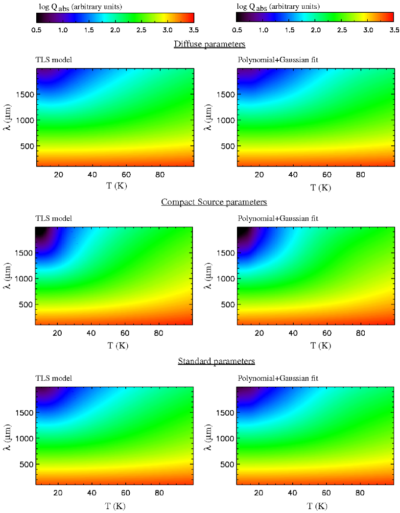
Figure 6: log $\rm Q_{abs}$ (in arbitrary units) as a function of temperature and wavelength derived from the TLS model (left panels) and from a polynomial+Gaussian fit performed on the TLS model (right panels), using different sets of parameters (from top to bottom: diffuse, compact sources, and standard).

Figure 5 shows two SEDs (one for an UCHII region and one for a cold clump) adjusted with the TLS model (using standard parameters) and T-$\beta$ models (using $\beta$=1.5; 2; and 2.5). For IRAS 19446+2505 (1) and CC6 (2), the temperatures reach from 30.2 K to 43.2 K and from 12.2 K to 18.2 K, depending on the model. Model fluxes after color correction, integrated into each band filter (squares in the figure), can be directly compared with the observational SEDs (diamonds in the figure). The 70 $\,{\rm\mu m}$ flux was not included in the fit for the cold clumps. While a T-$\beta$ model adopting a $\beta$ value of 1.5 is able reproduce the SED of the UCHII region, the same model gives a poor description of CC6 (2) SED, which requires a steeper spectrum ($\beta\simeq$2.5). The TLS model, however, describes each environment quite well by only changing the dust temperature. The main difference between the TLS and the T-$\beta$ model with a reasonable value of $\beta$ occurs in the mid-FIR ($\lambda<$70$\,{\rm\mu m}$) and in the mm range. But because of the large uncertainties in the Bolocam data, especially for cold clumps where the flux can be at the same level as the noise, the 1.1 mm flux does not add any strong constraints. However, even though in most cold clumps removing these data from the fits gives similar results, the 1.1 mm flux can also help the fit in some cases. Moreover, the 1.1 mm flux appears to have the same rough estimate as expected, which makes us confident in the use of these data.

In summary, each environment is characterized by a different dust emissivity index of the dust emission, which indicates distinct dust properties that leads to a change in $\beta$ for a T-$\beta$ model (from $\simeq$2-2.5 to 1.5, corresponding to warm and cold regions), or to a change in the TLS parameters (standard, diffuse, or CS parameters), for accurate descriptions of each type of environment. However, different from a T-$\beta$ model with a fixed $\beta$ that is not able to give good fits in warm as well as in cold regions, the standard TLS parameters can reproduce all types of environment reasonably well.

5.3 Simplifications of dust emission modeling

5.3.1 Polynomial fit on the TLS model

To facilitate using the TLS model predictions as a function of the environment, we performed a polynomial fit on the model, using the idl function sfit, for each set of parameters (diffuse, cold sources, and standard). This idl function allows us to determine a polynomial fit to a surface, which in our case is the dust absorption efficiency ($Q_{abs}$) deduced from the model as a function of temperature (6.9 K - 100 K) and wavelength (100 $\,{\rm\mu m}$ - 2 mm). However, for temperatures between 10 K and 15 K at wavelengths of around 2 mm, the difference between the model and the polynomial fit might become important. To minimize the difference we included a Gaussian function in the fit (using the idl function gauss2dfit). The final 2D function used to fit the model is then given as follows:

$$logQ_{abs}\left(\lambda,T\right)=\sum k_{j,i}\left((log\lambda-2.00076)/2.70167\times 10^{-3}\right)^{i}$$

$$\times\left((T-4.30000)/6.46369\times 10^{-1}\right)^{j}+a_{0}+a_{1}\times exp(\frac{-U}{2}),$$ (4)

with

$$U=\left(\frac{T-a_{4}}{a_{2}}\right)^{2}+\left(\frac{\lambda-a_{5}}{a_{3}}\right)^{2}.$$ (5)

Figure 7: Relative error (contours) between the polynomial+Gaussian fit and the TLS model $\left((Q_{abs,fit}-Q_{abs,model})/Q_{abs,model}\right)$ as a function of temperature and wavelength for the three sets of TLS parameters.

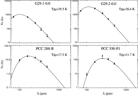
Figure 8: Herschel SEDs (diamonds) of two UCHII regions G29.1-0.0 and G29.2-0.0 from Paladini et al. (2012) and two cold cores PCC 288-B and PCC 550-P1 from Juvela et al. (2010). Polynomial+Gaussian fits of the TLS model are represented by the continuous line between 100 $\,{\rm\mu m}$ and 2 mm. Squares represent models integrated in the band filters of each instrument which allows direct comparisons with the data (diamonds).

The $k_{j,i}$ and $a$ coefficients are given in Tab. 5 and 6. The wavelength range is limited to 100 $\,{\rm\mu m}$ in the fits because for cold environments, emission at wavelengths below this limit can be contaminated by emission from small grains that are not in equilibrium with the radiation field. But since the polynomial fit is linear with wavelength in the FIR, that is, for $\lambda<300\,{\rm\mu m}$ in logarithmic scale, it can easily be extrapolated to shorter wavelengths if necessary. We found that a degree of 4 is adequate to achieve a reasonable fit on the TLS model. Plots of the TLS model and polynomial+Gaussian fits are presented in Fig. 6. Predictions of dust emission derived from the TLS model (proportional to $Q_{abs}$ values) as well as from the polynomial+Gaussian fit are given in arbitrary units, which means that they have to be normalized before they can be used. Reference values of emissivity or optical constants are given in the litterature, for instance, Boulanger et al. (1996) and Li $\&$ Draine (2001), which can then be converted into dust absorption efficiency. The normalization of the surface ($Q_{abs}$) to a reference value at some wavelength and temperature would lead to an easy determination of the dust column density of any observations in the framework of the TLS model. However, reference values of emissivity were determined for a given wavelength and for a specific temperature. The TLS model predicts emissivity variations as a function of wavelength and temperature. Predicted emissivities in the IRAS, Herschel, and Planck bands are given in Paradis et al. (2011) for different temperatures between 5 K and 100 K. Contours of the relative error $\left((Q_{abs,fit}-Q_{abs,model})/Q_{abs,model}\right)$ for each set of TLS parameters are given in Fig. 7. The 1-$\sigma$ standard deviation on the relative error is 3$\%$ over the entire ranges of temperatures and wavelengths for the CS parameters, and less than 2$\%$ for the diffuse and standard parameters. For all sets of parameters, absolute errors can also reach 10-12$\%$ at low temperature ($\sim 7$ K) in the submm and/or mm domain. We therefore encourage considering only temperatures higher than 7.5 K when using the polynomial+Gaussian fit. In addition, one has to be careful when using CS parameters: we note an increase in the errors when reaching long wavelengths (1750-2000 $\,{\rm\mu m}$), for temperatures around 10-15 K and an error of 10$\%$ for wavelengths between 700 $\,{\rm\mu m}$ and 950 $\,{\rm\mu m}$ and temperatures in the range 17 K - 20 K.

5.3.2 Universal application of the polynomial fit

The interest of the polynomial+Gaussian fit is to describe dust emission SEDs between 100 $\,{\rm\mu m}$ (or at shorter wavelengths by extrapolation when analyzing warm/hot dust grains) and 2 mm in any regions of our Galaxy. If the equilibrium dust temperature is known, it is easy to deduce the SED. In the opposite case, when the dust emission SED is known, it is then possible to determine the dust temperature. To check the applicability of this polynomial+Gaussian fit (performed on the TLS model with the use of the standard parameters), we compared the fit with known SEDs of UCHII regions (G29.1-0.0 and G29.2-0.0, from Paladini et al., 2012) and cold clumps (PCC 288-B and PCC 550-P1, from Juvela et al., 2010). Only the dust temperature in our fits varied from one SED to the other. Results are presented in Fig. 8. As we showed in Sect. 4.2.3, the determination of the dust temperature depends on the model used. Here, we did not perform any $\chi^{2}$ minimization. For G29.1-0.0 and G29.2-0.0, we used temperature values of 29.5 K and 26.4 K, which is close to the value of the cold component (29.5 K and 25.6 K) derived by Paladini et al. (2012) when using a two-component model with fixed dust emissivity index to minimize SEDs between 24 and 500 $\,{\rm\mu m}$. In these two regions the 70 $\,{\rm\mu m}$ emission is largely dominated by emission from the cold component. The polynomial+Gaussian fits were performed between 100 $\,{\rm\mu m}$ and 2 mm (see Sect. 5.3.1) and were extrapolated to 70 $\,{\rm\mu m}$ here, as shown in Fig. 8. For the cold clump PCC 550-P1, we considered a temperature of 11.7 K , which is close to the value of 11.3 K derived by Juvela et al. (2010) using a T-$\beta$ model with a deduced $\beta$ equal to 2.03. For PCC 288-B, the comparison between the polynomial+Gaussian fit and the SED is unsuitable when using the dust temperature derived from Juvela et al. (2010) (20.2 K), with a $\beta$ value found equal to 1.36. With the polynomial+Gaussian fit, a most appropriate value of dust temperature is around 17.5 K. We recall that the fits presented in Fig. 8 might be even better with the use of CC parameters in the polynomial+Gaussian fits for the cold clumps with the appropriate dust temperature. For PCC 550-P1, the fit is not able to reproduce the 250 $\,{\rm\mu m}$ flux, which could be due to calibration problems that have been improved since the first Herschel data. As reported in Juvela et al. (2010), a T-$\beta$ model is not able to match the 250 $\,{\rm\mu m}$ flux either.

We recall that model predictions essentially differ in the FIR and long wavelengths and also lead to different dust temperatures. For this reason, we encourage using the polynomial+Gaussian fit (or the TLS model), which does not bias the temperature estimate, but also takes the flattening of the spectra in the submm-mm domain into account, contrary to T-$\beta$ models. The TLS model predicts a more correct emissivity spectral behavior than any single fixed value of $\beta$ and precisely describes the emissivity spectral index as a function of temperature and wavelength (see Paradis et al., 2011, Fig. 6).

6 Conclusions

Using a combination of Herschel and Bolocam Galactic Plane surveys (Hi-GAL and BGPS) smoothed to a common resolution of 37^′′, we analyzed dust emission associated with two specific environments: UCHII regions and cold clumps. We studied twelve regions for each environment. We extracted SEDs in the central and the surrounding part of each region. We were able to compare the recent TLS model with emission spectra from warm dust ($\sim 30-40K$) in UCHII regions. We observed some variations in the dust optical properties with environments, as revealed by the change in the dust emissivity index, or in the set of TLS parameters that best fit the emission. In addition, contrary to any fixed value of the dust emissivity index (1.5, 2 and 2.5) that mostly fails to give good normalized $\chi^{2}$ in both warm environments such as UCHII regions and cold clump regions, the use of the standard TLS parameters can give reasonable results in all cases. These standard parameters were derived in a previous analysis to reproduce compact sources observed with Archeops and the diffuse medium as observed with FIRAS. Using a T-$\beta$ model for which the $\beta$ value is unknown can lead to an incorrect description of the dust emission. This comparison shows that the TLS model can easily be used to reliably predict dust emission spectra in any region of our Galaxy, in contrast to the T-$\beta$ model. We also reported an easy way to determine the emission at any temperature (in the range 7.5 K - 100 K) and wavelength (in the range 100 $\,{\rm\mu m}$ - 2 mm) for each set of TLS parameters by giving the 25 coefficients of a polynomial fit of degree 4, coupled with a Gaussian fit, which accurately reproduces the BG emission, after it is normalized to any reference value. The IDL code for the polynomial+Gaussian fit is available online.

Regions	$\chi^{2}_{TLS}$			Norm. $\chi^{2}_{TLS}$			$\chi^{2}_{T-\beta}$			Norm. $\chi^{2}_{T-\beta}$
	Diff.	CS	Std.	Diff.	CS	Std.	$\beta=2$	$\beta=1.5$	$\beta=2.5$	$\beta=2$	$\beta=1.5$	$\beta=2.5$
IRAS 17279-3350 (1)	0.801	0.974	0.805	0.822	1.000	0.826	1.074	0.426	2.351	1.103	0.437	2.414
IRAS 17279-3350 (2)	0.099	0.250	0.112	0.396	1.000	0.448	0.086	0.131	0.305	0.344	0.524	1.220
IRAS 17455-2800 (1)	0.061	0.112	0.062	0.545	1.000	0.554	0.211	0.166	1.170	1.884	1.482	10.446
IRAS 17455-2800 (2)	0.842	1.158	0.847	0.727	1.000	0.731	0.477	0.886	0.581	0.412	0.765	0.502
IRAS 17577-2320 (1)	0.804	0.745	0.775	1.000	0.927	0.964	1.327	0.341	2.814	1.650	0.424	3.500
IRAS 17577-2320 (2)	0.172	0.266	0.172	0.645	1.000	0.645	0.315	0.111	0.894	1.184	0.417	3.361
IRAS 18032-2032 (1)	1.237	1.377	1.177	0.898	1.000	0.855	2.106	1.008	4.421	1.529	0.732	3.211
IRAS 18032-2032 (2)	0.408	0.911	0.448	0.448	1.000	0.492	0.049	0.373	0.191	0.054	0.409	0.210
IRAS 18116-1646 (1)	0.233	0.343	0.217	0.679	1.000	0.633	0.686	0.065	2.480	2.000	0.190	7.230
IRAS 18116-1646 (2)	0.336	0.956	0.389	0.351	1.000	0.407	0.059	0.294	0.378	0.062	0.308	0.395
IRAS 18317-0757 (1)	0.234	0.561	0.290	0.417	1.000	0.517	0.088	0.485	0.397	0.157	0.865	0.708
IRAS 18317-0757 (2)	0.288	0.443	0.291	0.650	1.000	0.657	0.296	0.239	0.741	0.668	0.539	1.673
IRAS 18434-0242 (1)	4.016	3.966	3.922	1.000	0.988	0.977	5.029	4.032	6.590	1.252	1.004	1.641
IRAS 18434-0242 (2)	0.069	0.131	0.068	0.527	1.000	0.519	0.075	0.130	0.297	0.573	0.992	2.267
IRAS 18469-0132 (1)	1.217	1.407	1.204	0.865	1.000	0.858	1.833	0.519	4.200	1.303	0.369	2.985
IRAS 18469-0132 (2)	0.041	0.118	0.048	0.347	1.000	0.407	0.100	0.066	0.250	0.847	0.559	2.119
IRAS 18479-0005 (1)	2.087	1.968	1.983	1.000	0.943	0.950	3.345	1.578	6.143	1.603	0.756	2.943
IRAS 18479-0005 (2)	0.371	0.700	0.396	0.530	1.000	0.566	0.082	0.443	0.165	0.117	0.633	0.236
IRAS 18502+0051 (1)	1.160	1.498	1.158	0.774	1.000	0.773	1.576	0.642	3.988	1.052	0.429	2.662
IRAS 18502+0051 (2)	0.052	0.073	0.050	0.712	1.000	0.684	0.096	0.136	0.483	1.315	1.863	6.616
IRAS 19442+2427 (1)	2.134	2.046	2.061	1.000	0.959	0.966	3.285	1.117	6.391	1.539	0.523	2.995
IRAS 19442+2427 (2)	0.131	0.302	0.143	0.434	1.000	0.474	0.039	0.224	0.231	0.129	0.742	0.765
IRAS 19446+2505 (1)	0.249	0.301	0.211	0.827	1.000	0.701	1.121	0.123	3.275	3.724	0.409	10.880
IRAS 19446+2505 (2)	0.111	0.512	0.151	0.217	1.000	0.295	0.091	0.055	0.386	0.178	0.107	0.754
Total nb. of best $\chi^{2}$	-	-	-	13 (52$\%$)	3 (12$\%$)	9 (36$\%$)	-	-	-	9 (37.5$\%)$	15 (62.5$\%$)	0 (0$\%$)
Total $\chi^{2}$	-	-	-	15.811	23.817	15.899	-	-	-	24.679	15.478	71.733
Cold clump 1 (1)	0.017	0.021	0.017	0.810	1.000	0.810	0.017	0.027	0.026	0.810	1.286	1.238
Cold clump 1 (2)	0.002	0.068	0.008	0.029	1.000	0.117	0.011	0.030	0.088	0.162	0.441	1.294
Cold clump 2 (1)	0.019	0.036	0.015	0.528	1.000	0.417	0.021	0.047	0.101	0.583	1.306	2.806
Cold clump 2 (2)	0.037	0.104	0.031	0.356	1.000	0.298	0.030	0.115	0.121	0.288	1.106	1.163
Cold clump 3 (1)	0.014	0.001	0.009	1.000	0.071	0.643	0.008	0.045	0.001	0.571	3.214	0.071
Cold clump 3 (2)	0.551	0.170	0.441	1.000	0.301	0.800	0.305	1.045	0.062	0.553	1.897	0.113
Cold clump 4 (1)	0.007	0.023	0.006	0.304	1.000	0.261	0.008	0.029	0.023	0.348	1.261	1.000
Cold clump 4 (2)	0.255	0.022	0.185	1.000	0.086	0.725	0.147	0.701	0.021	0.576	2.749	0.082
Cold clump 5 (1)	0.028	0.003	0.019	1.000	0.107	0.679	0.020	0.090	0.003	0.714	3.214	0.107
Cold clump 5 (2)	0.270	0.026	0.200	1.000	0.096	0.741	0.188	0.556	0.023	0.696	2.059	0.085
Cold clump 6 (1)	0.243	0.056	0.200	1.000	0.230	0.823	0.216	0.427	0.098	0.889	1.757	0.403
Cold clump 6 (2)	0.169	0.015	0.114	1.000	0.089	0.675	0.121	0.422	0.014	0.716	2.497	0.083
Cold clump 7 (1)	0.099	0.119	0.097	0.832	1.000	0.815	0.103	0.103	0.128	0.866	0.866	1.076
Cold clump 7 (2)	0.121	0.025	0.076	1.000	0.207	0.628	0.030	0.438	0.188	0.248	3.620	1.554
Cold clump 8 (1)	0.066	0.027	0.058	1.000	0.409	0.879	0.058	0.106	0.033	0.879	1.606	0.500
Cold clump 8 (2)	0.932	0.055	0.679	1.000	0.059	0.729	0.639	2.028	0.080	0.686	2.176	0.086
Cold clump 9 (1)	0.049	0.102	0.033	0.480	1.000	0.324	0.033	0.166	0.184	0.323	1.627	1.804
Cold clump 9 (2)	0.351	0.100	0.266	1.000	0.285	0.758	0.238	0.658	0.100	0.678	1.875	0.285
Cold clump 10 (1)	0.042	0.040	0.042	1.000	0.952	1.000	0.042	0.052	0.043	1.000	1.238	1.024
Cold clump 10 (2)	0.254	0.071	0.189	1.000	0.280	0.744	0.053	0.604	0.088	0.209	2.378	0.346
Cold clump 11 (1)	0.010	0.008	0.007	1.000	0.800	0.700	0.009	0.018	0.009	0.900	1.800	0.900
Cold clump 11 (2)	0.264	0.099	0.203	1.000	0.375	0.769	0.189	0.595	0.095	0.716	2.254	0.360
Cold clump 12 (1)	0.064	0.094	0.056	0.681	1.000	0.596	0.065	0.111	0.103	0.691	1.181	1.100
Cold clump 12 (2)	0.039	0.055	0.024	0.710	1.000	0.436	0.022	0.180	0.027	0.400	3.273	0.490
Total nb. of best $\chi^{2}$	-	-	-	2 (8$\%$)	14 (56$\%$)	9 (36$\%$)	-	-	-	12 (48$\%$)	1 (4$\%$)	12 (48$\%$)
Total $\chi^{2}$	-	-	-	19.730	13.347	15.367	-	-	-	14.502	46.681	17.970

Table 7: Reduced $\chi^{2}$ derived from fits between Herschel-Bolocam data and TLS and T-$\beta$ modeling using different sets of parameters (diffuse, compact sources, and standard parameters, columns 2, 3, and 4, respectively) and $\beta$ values (2, 1.5, and 2.5, columns 8, 9, and 10). Values of reduced $\chi^{2}$ presented in columns 5, 6, 7 and 11, 12, 13 are normalized with respect to the highest $\chi^{2}$ value derived from the TLS model.

References

- Anderson et al. (1972) Anderson, P. W., Halperin, B. I., Varma, C. M. 1972, Phil. Mag., 25, 1
- Aguirre et al. (2011) Aguirre, J. E., Ginsburg, A. G., Dunham, M. K., et al. 2011, ApJS, 192, 4
- Bally et al. (2010) Bally, J., Aguirre, J., Battersby, C., et al. 2010, ApJ, 721, 137
- Bernard et al. (2010) Bernard, J.-P., Paradis, D., Marshall, D. J. 2010, AA, 581L, 88
- Boudet et al. (2005) Boudet, N., Mutschke, H., Nayral, C., et al. 2005, ApJ, 633, 272
- Boulanger et al. (1996) Boulanger, F., Abergel, A., Bernard, J.-P., et al. 1996, AA, 312, 256
- Carey et al. (2009) Carey, S. J., Noriega-Crespo, A., Mizuno, D. R., et al. 2009, PASP, 121, 76
- Codella et al. (1994) Codella, C., Felli, M. Natale, V. 1994, AA, 284, 233
- Compiègne et al. (2011) Compiègne, M., Verstreate, L., Jones, A., et al. 2011, AA, 525, 103
- Coupeaud et al. (2011) Coupeaud, A., Demyk, K., Mény, C., et al. 2011, AA, 535, 124
- Désert et al. (2008) Désert, F.-X., Macías-Pérez, J. F., Mayet, F., et al. 2008, AA, 481, 411
- Draine Lee (1984) Draine, B. T. Lee, H. M. 1984, ApJ, 285, 89
- Dupac et al. (2003) Dupac, X., Bernard, J.-Ph., Boudet, N., et al. 2003, AA, 404, L11
- Finkbeiner et al. (1999) Finkbeiner, D., P., Davis, M., Schlegel, D. J. 1999, ApJ, 524, 867
- Galliano et al. (2005) Galliano, F., Madden, S. C., Jones, A., et al. 2005, AA, 434, 867
- Galliano et al. (2011) Galliano, F., Hony, S., Bernard, J.-P., et al. 2011, AA, 536, 88
- Ginsburg et al. (2013) Ginsburg, A., Glenn, J., Rosolowsky, E., et al. 2013, ApJS, 208, 14
- Gordon et al. (2010) Gordon, K., Galliano, F., Hony, S., et al. 2010, AA, 518L, 89
- Gordon et al. (2014) Gordon, K., Roman-Duval, J., Bot, C., et al. 2014, arXiv1406.7469
- Jackson et al. (2006) Jackson, J. M., Rathborne, J. M., Shah, R. Y., et al. 2006, ApJS, 163, 145
- Juvela et al. (2010) Juvela, M., Ristorcelli, I., Montier, L., et al. 2010, AA, 518, L93
- Juvela et al. (2013) Juvela, M., Montillaud, J., Ysard, N., Lunttila, T. 2013, AA, 556, 63
- Kelly et al. (2012) Kelly, B. C., Shetty, R., Stutz, A. M., et al. 2012, ApJ, 752, 55
- Kiuchi et al. (2004) Kiuchi, G., Ohta, K., Sawicki, M., Allen, M. 2004, AJ, 128, 2743
- Kohler et al. (2011) Kohler, M., Guillet, V., Jones, A. 2011, AA, 528, 96
- Kohler et al. (2012) Kohler, M., Stepnik, B., Jones, A., et al. 2012, AA, 548, 61
- Li Draine (2001) Li, A., Draine, B. 2001, ApJ, 554, 778
- Marshall et al. (2013) Marshall, D. J., et al. 2013, AA, in prep.
- Mennella et al. (1998) Mennella, V., Brucato, J. R., Colangeli, L., et al. 1998, ApJ, 496, 1058
- Mény et al. (2007) Mény, C., Gromov, V., Boudet, N., et al. 2007, AA, 468, 171
- Miville-Deschênes Lagache (2005) Miville-Deschênes, M. A., Lagache, G. 2005, ApJS, 157, 302
- Molinari et al. (2010a) Molinari, S., Swinyard, B., Bally, J., et al. 2010a, PASP, 122, 314
- Molinari et al. (2010b) Molinari, S., Swinyard, B., Bally, J., et al. 2010b, AA, 518, 100
- Paladini et al. (2007) Paladini, R., Montier, L., Giard, M., et al. 2007, AA, 465, 839
- Paladini et al. (2012) Paladini, R., Umana, G., Veneziani, M., et al. 2012, ApJ, 760, 149
- Paradis et al. (2009) Paradis, D., Bernard, J.-P, Mény, C. 2009, AA, 506, 745
- Paradis et al. (2010) Paradis, D., Veneziani, M., Noriega-Crespo, A., et al. 2010, AA, 520, L8
- Paradis et al. (2011) Paradis, D., Bernard, J.-P., Mény, C., Gromov, V. 2011, A A, 534, 118
- Paradis et al. (2012) Paradis, D., Paladini, R., Noriega-Crespo, A., et al. 2012, AA, 537, 113
- Peeters et al. (2002) Peeters, E., Martin-Hernandez, N. L., Damour, F., et al. 2002, AA, 381, 571
- Phillips (1972) Phillips, W. 1972, J. Low Temp. Phys., 11, 757
- Phillips (1987) Phillips, W. 1987,Rep. Prog. Phys., 50, 1657
- Planck Collaboration (2011) Planck Collaboration 2011, AA, 536, 23
- Planck Collaboration (2014) Planck Collaboration 2014, AA, 564, 45
- Poglitsch et al. (2010) Poglitsch, A., Waelkens, C., Geis, N., et al. 2010, AA, 518, 2
- Reach et al. (1995) Reach, W.T., Dwek, E., Fixsen, D.J., Hewagama, T. et al., 1995, ApJ, 451, 188
- Schlomann (1964) Schlomann, E. 1964, Phys. Rev., 135, 413
- Schnee et al. (2010) Schnee, S., Enoch, M., Noriega-Crespo, A., et al. 2010, ApJ, 708, 127
- Shetty et al. (2009) Shetty, R., Kauffmann, J., Schnee, S., et al. 2009, ApJ, 696, 2234
- Stepnik et al. (2003) Stepnik, B., Abergel, A., Bernard, J.-P., et al. 2003, AA, 398, 551
- Traficante et al. (2011) Traficante, A., Calzoletti, L., Veneziani, M., et al. 2011, MNRAS, 416, 2932
- Veneziani et al. (2010) Veneziani, M., Ade, P. A. R., Bock, J. J., et al. ApJ, 2010, 713, 959
- Veneziani et al. (2013) Veneziani, M., Piacentini, F., Noriega-Crespo, A., et al. ApJ, 2013, 772, 56
- Vinogradov (1960) Vinogradov, V. S. 1960, Fiz. Tverd. Tela, 2, 2622 (English transl. 1961, Sov. Phys. Solid St. 2, 2338)
- Wood Churchwell (1989a) Wood, D. O. S., Churchwell, E. 1989a, ApJ, 340, 265
- Wood Churchwell (1989b) Wood, D. O. S., Churchwell, E. 1989b, ApJS, 69, 831