Wave Propagation through an Array of Slits

Abstract

Propagation of a wave through an array of slits is theoretically investigated. The asymptotic expansion of the matrix elements of the propagation operator is derived and compared with numerical calculations. And then the eigenmodes and eigenvalues of the propagation operator are estimated. Our analysis should provide an insight into the properties of waveguides composed of opaque masks that have been proposed recently.

1 Introduction

A new type of waveguides composed of opaque masks (slits or pinholes) has recently been proposed[1, 2]. In this waveguide a wave propagates through a set of identical masks that are aligned on a straight line with equal spacing (see fig.1 for the case of slit array). The peculiarity of this waveguide is that no special material is required for its construction (transparency, high reflectivity, …). One possible application of such waveguides is to integrate light waveguides on a silicon chip. It can also be used to guide matter waves. In analyzing the wave propagation in such waveguides, a continuous model has been used [1, 2, 3, 4]. In this model, the discrete set of opaque masks that constitutes the waveguide is replaced with a continuous absorbing medium that has a hole with a cross section identical to the opening of the masks. This model predicts that the attenuation per unit length of the wave propagating in the waveguide is proportional to the square root of the spacing $L$ between the masks, so that it can be decreased by reducing $L$. Though it is known that this model reproduces the experimental results reasonably, the physical ground of replacing the discrete set of masks with a continuous medium is not very clear. In this paper we consider the wave propagation in an array of slits and treat the discrete set of slits directly. We first calculate the asymptotic expansion of the matrix elements of the propagation operator which is then compared with the numerical calculations given in the appendix. From these results we deduce the eigenmodes and eigenvalues of the propagation operator.

2 Theoretical model

Suppose a monochromatic wave of a wavenumber $k_{c}$ is propagating through an array of slits as depicted in fig.1. We assume that the opening of slits are much larger then the wavelength of the wave. We look for the evolution of the transverse wavefunction $\varphi(x)$.

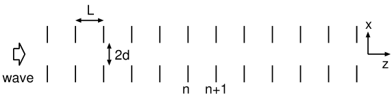
Figure 1: Slit array. Identical slits of opening $2d$ (full width) are aligned on a straight line with spacing $L$ between the slits. $d\gg\lambda\,(\equiv\frac{2\pi}{k_{c}})$ is assumed.

The propagation process is divided into two parts: free propagation $F$ between the two neighbouring slits (for length $L$) and masking $M$ of the transverse wavefunction by the slit. We shall denote the position just after the $n$th slit $P_{n}$. Then, the propagation operator $T$ corresponding to the propagation of the wave from the position $P_{n}$ to $P_{n+1}$ is written as $T=MF$. The masking operator $M$ just masks the transverse wavefunction:

$$(M\varphi)(x)=\left\{\begin{array}[]{ll}\varphi(x)&(|x|<d)\\ 0&(|x|\geq d)\end{array}\right..$$ (1)

The transverse wavefunction $\varphi(x)$ just after a slit takes nonzero value only inside the opening of the slit (i.e. $-d<x<d$). Such subspace of wavefunctions is spanned by a set of orthonormal basis functions:

$$\varphi_{m}(x)\equiv\left\{\begin{array}[]{ll}\frac{1}{\sqrt{d}}\sin\frac{(m+1)\pi}{2d}(x+d)&(-d<x<d)\\ 0&(|x|\geq d)\end{array}\right.\ \ \ (m=0,1,2,...)$$ (2)

We calculate the matrix elements of $T$ using this basis. Since $M$ has no effect on this basis functions (i.e. $M\varphi_{m}=\varphi_{m}$), $\langle\varphi_{m}|T|\varphi_{n}\rangle=\langle\varphi_{m}|F|\varphi_{n}\rangle$.

3 Propagation operator $T$

For a transverse wavefunction that has a transverse wavenumber $k_{x}$, the possible values that the longitudinal wavenumber $k_{z}$ can take are $\pm\sqrt{k_{c}^{2}-k_{x}^{2}}$. Here we choose only $k_{z}=\sqrt{k_{c}^{2}-k_{x}^{2}}$, i.e. we neglect the process of multiple scattering of the wave between slits in which the wave sometimes propagates backward (i.e. in $-z$ direction). Thus $F|k_{x}\rangle=\exp\left(i\sqrt{k_{c}^{2}-k_{x}^{2}}L\right)|k_{x}\rangle$. From the assumption that $d\gg\lambda$, the wavenumber component of $\varphi_{m}$ is concentrated in the region $|k_{x}|\ll k_{c}$ so that $\sqrt{k_{c}^{2}-k_{x}^{2}}\fallingdotseq k_{c}-\frac{k_{x}^{2}}{2k_{c}}$ (paraxial approximation), and thus $F|k_{x}\rangle=\exp(-i\alpha k_{x}^{2})|k_{x}\rangle$ with $\alpha\equiv\frac{L}{2k_{c}}$ (we omit the global phase factor $\exp(ik_{c}L)$ hereafter). The matrix elements $T_{mn}=\langle\varphi_{m}|T|\varphi_{n}\rangle$ is calculated as

$$\begin{array}[]{rl}T_{mn}=&\langle\varphi_{m}|F|\varphi_{n}\rangle\\ =&\int_{-\infty}^{\infty}dk_{x}\,\langle\varphi_{m}|F|k_{x}\rangle\langle k_{x}|\varphi_{n}\rangle\\ =&\int_{-\infty}^{\infty}dk_{x}\,\langle\varphi_{m}|k_{x}\rangle\exp\left(-i\alpha k_{x}^{2}\right)\langle k_{x}|\varphi_{n}\rangle\end{array}$$ (3)

with

$$\begin{array}[]{ll}\langle\varphi_{m}|k_{x}\rangle&=\int_{-\infty}^{\infty}dx\,\varphi_{m}(x)\langle x|k_{x}\rangle\\ &=\int_{-d}^{d}dx\,\frac{1}{\sqrt{d}}\sin k_{m}(x+d)\frac{1}{\sqrt{2\pi}}e^{ik_{x}x}\\ &=\frac{k_{m}}{\sqrt{2\pi d}}\left\{(-1)^{m+1}e^{ik_{x}d}-e^{-ik_{x}d}\right\}\frac{1}{k_{x}^{2}-k_{m}^{2}}\end{array}$$ (4)

where $k_{m}\equiv\frac{(m+1)\pi}{2d}$.

4 Matrix elements $T_{mn}$

Now we calculate the asymptotic expansion of the matrix elements $T_{mn}$ of the propagation operator $T$. From (3) and (4), $T_{mn}$ is calculated as

$$\begin{array}[]{rl}T_{mn}=&\frac{k_{m}k_{n}}{2\pi d}\int_{-\infty}^{\infty}dk_{x}\frac{1}{k_{x}^{2}-k_{m}^{2}}\frac{1}{k_{x}^{2}-k_{n}^{2}}\\ &\ \ \{1+(-1)^{m+n}+(-1)^{m}e^{2ik_{x}d}+(-1)^{n}e^{-2ik_{x}d}\}e^{-i\alpha k_{x}^{2}}\\ \end{array}$$ (5)

In the following, we consider only the case when $(-1)^{m}=(-1)^{n}$, because otherwise $T_{mn}=0$. (5) is rewritten using a new variable $u=\sqrt{\alpha}k_{x}$ as

$$\begin{array}[]{rl}T_{mn}=&\frac{v_{m}v_{n}}{2\pi}\int_{-\infty}^{\infty}\nu^{3}du\frac{1}{u^{2}-\nu^{2}v_{m}^{2}}\frac{1}{u^{2}-\nu^{2}v_{n}^{2}}\\ &\ \ \times\{2+(-1)^{m}e^{2i\frac{u}{\nu}}+(-1)^{n}e^{-2i\frac{u}{\nu}}\}e^{-iu^{2}}\\ \end{array}$$ (6)

with $v_{m}\equiv k_{m}d=\frac{(m+1)\pi}{2}$ and $\nu=\frac{\sqrt{\alpha}}{d}=\sqrt{\frac{L}{2k_{c}d^{2}}}=\frac{1}{2\sqrt{\pi}}\left(\frac{\lambda L}{d^{2}}\right)^{\frac{1}{2}}$. Hereafter we assume that $\frac{\lambda L}{d^{2}}\ll 1$ (and thus $\nu\ll 1$) in which case, as we shall see, the loss of the propagation is small. Because the integrand has no pole anywhere, we can change the integration path from $P_{0}$ to $P_{1}$ (see fig.2), and then divide the integrand into 3 parts. As a consequence, poles appear at $u=\pm\nu v_{m}$ and $u=\pm\nu v_{n}$.

$$\begin{array}[]{rl}T_{mn}=&\frac{v_{m}v_{n}}{2\pi}\int_{P_{1}}\nu^{3}du\frac{1}{u^{2}-\nu^{2}v_{m}^{2}}\frac{1}{u^{2}-\nu^{2}v_{n}^{2}}\\ &\ \ \times\{\underbrace{2}_{A}+\underbrace{(-1)^{m}e^{2i\frac{u}{\nu}}}_{B+}+\underbrace{(-1)^{n}e^{-2i\frac{u}{\nu}}}_{B-}\}e^{-iu^{2}}\\ \end{array}$$ (7)

Now we change the integration path from $P_{1}$ to $P_{2}$.

The case $m\neq n$

$$\begin{array}[]{rl}T_{mn}=&\frac{v_{m}v_{n}}{2\pi(v_{m}^{2}-v_{n}^{2})}\int_{P_{2}}du\left(\frac{\nu}{u^{2}-\nu^{2}v_{m}^{2}}-\frac{\nu}{u^{2}-\nu^{2}v_{n}^{2}}\right)\\ &\ \ \{\underbrace{2}_{A}+\underbrace{(-1)^{m}e^{2i\frac{u}{\nu}}}_{B+}+\underbrace{(-1)^{n}e^{-2i\frac{u}{\nu}}}_{B-}\}e^{-iu^{2}}\\ =&I_{A}+I_{B+}+I_{B-}\end{array}$$ (8)

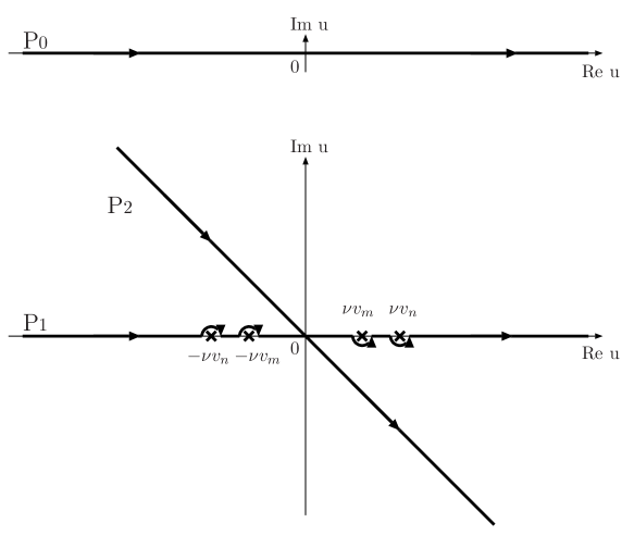
Figure 2: Integration path for evaluating $T_{mn}$ (see text).

By defining

$$I_{1}(\gamma)\equiv\int_{P_{2}}\frac{e^{-iu^{2}}}{u^{2}-\gamma}du$$ (9)

and

$$I_{1\pm}(\gamma,\beta)\equiv\int_{P_{2}}\frac{e^{\pm 2i\beta u}e^{-iu^{2}}}{u^{2}-\gamma}du,$$ (10)

$I_{A}$ and $I_{B\pm}$ are written as

$$I_{A}=\frac{v_{m}v_{n}}{\pi(v_{m}^{2}-v_{n}^{2})}\nu\{I_{1}(\nu^{2}v_{m}^{2})-I_{1}(\nu^{2}v_{n}^{2})\}$$ (11)

$$I_{B\pm}=(-1)^{m}\frac{v_{m}v_{n}}{2\pi(v_{m}^{2}-v_{n}^{2})}\nu\left\{I_{1\pm}\left(\nu^{2}v_{m}^{2},\frac{1}{\nu}\right)-I_{1\pm}\left(\nu^{2}v_{n}^{2},\frac{1}{\nu}\right)\right\}$$ (12)

Taking a variable $s$ as $u=\sqrt{-i}\,s$,

$$\begin{array}[]{ll}I_{1}(\gamma)&=\sqrt{i}\int_{-\infty}^{\infty}\frac{e^{-s^{2}}}{s^{2}-i\,\gamma}\,ds\\ &=\sqrt{i}e^{-i\gamma}\int_{-\infty}^{\infty}\int_{1}^{\infty}e^{-(s^{2}-i\gamma)s^{\prime}}\,ds^{\prime}\,ds\\ &=\sqrt{\pi i}\,e^{-i\gamma}\int_{1}^{\infty}\frac{e^{i\gamma s^{\prime}}}{\sqrt{s^{\prime}}}\,ds^{\prime}\\ &=2\sqrt{\pi i}\,e^{-i\gamma}\left\{\int_{0}^{\infty}e^{i\gamma s^{\prime\prime 2}}\,ds^{\prime\prime}-\int_{0}^{1}e^{i\gamma s^{\prime\prime 2}}\,ds^{\prime\prime}\right\}\\ &=\sqrt{\pi i}\,e^{-i\gamma}\sqrt{\frac{\pi}{-i\gamma}}\left\{1-{\rm erf}(\sqrt{-i\gamma})\right\}\\ &=e^{-i\gamma}\left\{\frac{\pi i}{\sqrt{\gamma}}-2\sqrt{\pi i}\sum_{n=0}^{\infty}\frac{1}{2n+1}\frac{(i\gamma)^{n}}{n!}\right\}\\ &=e^{-i\gamma}\frac{\pi i}{\sqrt{\gamma}}-2\sqrt{\pi i}\sum_{n=0}^{\infty}\frac{(-2i\gamma)^{n}}{(2n+1)!!}\end{array}$$ (13)

where ${\rm erf}$ is the error function defined by

$${\rm erf}(z)\equiv\frac{2}{\sqrt{\pi}}\int_{0}^{z}e^{-t^{2}}dt=\frac{2}{\sqrt{\pi}}\left(z-\frac{z^{3}}{3}+\frac{z^{5}}{10}-\frac{z^{7}}{42}+...\right).$$ (14)

The formula used to derive the series expansion of the last line of (13) is presented in the appendixB. To evaluate $I_{1\pm}(\gamma,\beta)$, the integration path is changed from $P_{2}$ to $P_{r\pm}+P_{p\pm}$ (fig.3):

$$I_{1\pm}(\gamma,\beta)=\int_{P_{r\pm}+P_{p\pm}}\frac{e^{\pm 2i\beta u}e^{-iu^{2}}}{u^{2}-\gamma}du=I_{1r\pm}(\gamma,\beta)+I_{1p\pm}(\gamma,\beta)$$ (15)

$I_{1r\pm}(\gamma,\beta)$ is calculated by evaluating the residue of the integrand at $u=\pm\sqrt{\gamma}$ giving

$$I_{1r\pm}(\gamma,\beta)=\pi i\frac{e^{2i\beta\sqrt{\gamma}}e^{-i\gamma}}{\sqrt{\gamma}}$$ (16)

To evaluate $I_{1p\pm}(\gamma,\beta)$, we take a variable $s$ as $u=\sqrt{-i}\,s\pm\beta$ so that

$$I_{1p\pm}(\gamma,\beta)=\sqrt{i}\,e^{i\beta^{2}}\int_{-\infty}^{\infty}\frac{e^{-s^{2}}}{(s\pm\sqrt{i}\beta)^{2}-\gamma}ds$$ (17)

We now assume that $|\gamma|\ll 1$ and $|\beta|\gg 1$ (because $I_{1\pm}$ is used in the form (12) and $\nu\ll 1$) so that $I_{1p\pm}$ can be expanded as

$$I_{1p\pm}(\gamma,\beta)=\sqrt{i}\,e^{i\beta^{2}}\sum_{n=0}^{\infty}g_{n\pm}(\beta)\,\gamma^{n}$$ (18)

with

$$g_{n\pm}(\beta)\equiv\int_{-\infty}^{\infty}\frac{e^{-s^{2}}}{(s\pm\sqrt{i}\beta)^{2(n+1)}}\,ds=\frac{(-i)^{n+1}\sqrt{\pi}}{\beta^{2(n+1)}}+...$$ (19)

Terms that appear in the right-hand sides of (11) and (12) are evaluated as

$$I_{1}(\nu^{2}v_{m}^{2})=e^{-i\nu^{2}v_{m}^{2}}\frac{\pi\,i}{\nu v_{m}}-2\sqrt{\pi i}\sum_{n=0}^{\infty}\frac{(-2i\,\nu^{2}v_{m}^{2})^{n}}{(2n+1)!!}$$ (20)

$$I_{1r\pm}\left(\nu^{2}v_{m}^{2},\frac{1}{\nu}\right)=\pi i\frac{(-1)^{m+1}e^{-i\nu^{2}v_{m}^{2}}}{\nu v_{m}}$$ (21)

Now we are ready to evaluate $T_{mn}$. The contribution of the first term of $I_{1}$ cancels with the contribution of $I_{1r\pm}$.

$$\begin{array}[]{ll}T_{mn}&=\frac{v_{m}v_{n}}{\pi}\nu(-2\sqrt{\pi i})\sum_{n=1}^{\infty}\frac{(-2i\,\nu^{2})^{n}}{(2n+1)!!}\frac{v_{m}^{2n}-v_{n}^{2n}}{v_{m}^{2}-v_{n}^{2}}+T_{osc}\\ &=-4\sqrt{\frac{-i}{\pi}}v_{m}v_{n}\nu^{3}\sum_{n=1}^{\infty}\frac{(-2i\,\nu^{2})^{n-1}}{(2n+1)!!}\frac{v_{m}^{2n}-v_{n}^{2n}}{v_{m}^{2}-v_{n}^{2}}+T_{osc}\\ &=-\frac{4}{3}\sqrt{\frac{-i}{\pi}}v_{m}v_{n}\nu^{3}\left(1+\frac{-2i\nu^{2}}{5}\frac{v_{m}^{4}-v_{n}^{4}}{v_{m}^{2}-v_{n}^{2}}+\frac{(-2i\nu^{2})^{2}}{35}\frac{v_{m}^{6}-v_{n}^{6}}{v_{m}^{2}-v_{n}^{2}}+...\right)+T_{osc}\end{array}$$ (22)

The term $T_{osc}$ is the contribution from $I_{p\pm}$ and oscillates rapidly as $e^{i\beta^{2}}=e^{i\nu^{-2}}$ when $\nu\to 0$. Its leading term is proportional to $\nu^{7}$ in magnitude:

$$T_{osc}=\sqrt{\frac{-i}{\pi}}v_{m}v_{n}e^{i\nu^{-2}}\nu^{7}\left\{1+O(\nu)\right\}$$ (23)

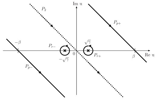
Figure 3: Integration path to evaluate $I_{1}(\nu)$ and $I_{1\pm}(\nu,\beta)$ (see text).

The case $m=n$

$$\begin{array}[]{rl}T_{mm}=&\frac{v_{m}^{2}}{2\pi}\int_{-\infty}^{\infty}\nu^{3}du\left(\frac{1}{u^{2}-\nu^{2}v_{m}^{2}}\right)^{2}\{\underbrace{2}_{A}+\underbrace{(-1)^{m}e^{2i\frac{u}{\nu}}}_{B+}+\underbrace{(-1)^{m}e^{-2i\frac{u}{\nu}}}_{B-}\}e^{-iu^{2}}\\ =&I_{A}+I_{B+}+I_{B-}\end{array}$$ (24)

By defining

$$I_{2}(\gamma)\equiv\int_{P_{2}}\frac{e^{-iu^{2}}}{(u^{2}-\gamma)^{2}}du$$ (25)

and

$$I_{2\pm}(\gamma,\beta)\equiv\int_{P_{2}}\frac{e^{\pm 2i\beta u}e^{-iu^{2}}}{(u^{2}-\gamma)^{2}}du,$$ (26)

$I_{A}$ and $I_{B\pm}$ are written as

$$I_{A}=\frac{v_{m}^{2}}{\pi}\,\nu^{3}I_{2}(\nu^{2}v_{m}^{2})$$ (27)

and

$$I_{B\pm}=(-1)^{m}\frac{v_{m}^{2}}{2\pi}\,\nu^{3}I_{2\pm}\left(\nu^{2}v_{m}^{2},\frac{1}{\nu}\right)$$ (28)

where $I_{2}$ and $I_{2\pm}$ are evaluated from $I_{1}$ and $I_{1\pm}$ as follows:

$$I_{2}(\gamma)=I_{1}^{\prime}(\gamma)= \partial_{\gamma}\left(e^{-i\gamma}\frac{\pi i}{\sqrt{\gamma}}\right)-4\sqrt{-\pi i}\,e^{-i\gamma}\sum_{n=0}^{\infty}\frac{1}{(2n+1)(2n+3)}\frac{(i\gamma)^{n}}{n!}$$ (29a)

$$= \partial_{\gamma}\left(e^{-i\gamma}\frac{\pi i}{\sqrt{\gamma}}\right)-4\sqrt{-\pi i}\sum_{n=0}^{\infty}(n+1)\frac{(-2i\gamma)^{n}}{(2n+3)!!}$$ (29b)

$$I_{2\pm}(\gamma,\beta)=\partial_{\gamma}I_{1\pm}(\gamma,\beta)=I_{2r\pm}(\gamma,\beta)+I_{2p\pm}(\gamma,\beta)$$ (30)

Here $I_{2r\pm}$ and $I_{2p\pm}$ are defined as

$$I_{2r\pm}(\gamma,\beta)\equiv \partial_{\gamma}I_{1r\pm}(\gamma,\beta)= e^{2i\beta\sqrt{\gamma}}\partial_{\gamma}\left(e^{-i\gamma}\frac{\pi i}{\sqrt{\gamma}}\right)-\frac{\pi\beta}{\gamma}e^{2i\beta\sqrt{\gamma}}e^{-i\gamma}$$ (31)

$$I_{2p\pm}(\gamma,\beta)\equiv \partial_{\gamma}I_{1p\pm}(\gamma,\beta)= \sqrt{-\pi i}e^{i\beta}\frac{1}{\beta^{4}}+...$$ (32)

Finally $T_{mm}$ is calculated as

$$T_{mm}= e^{-i\nu^{2}v_{m}^{2}}\left\{1-4\sqrt{\frac{-i}{\pi}}\nu^{3}v_{m}^{2}\sum_{n=0}^{\infty}\frac{1}{(2n+1)(2n+3)}\frac{(i\nu^{2}v_{m}^{2})^{n}}{n!}\right\}+T_{osc}$$ (33a)

$$= e^{-i\nu^{2}v_{m}^{2}}-4\sqrt{\frac{-i}{\pi}}\nu^{3}v_{m}^{2}\sum_{n=0}^{\infty}(n+1)\frac{(-2i\nu^{2}v_{m}^{2})^{n}}{(2n+3)!!}+T_{osc}$$ (33b)

where the leading term of the oscillating term $T_{osc}$ is same as in (23) with $n=m$. $T_{mn}$ up to the order of $O(\nu^{4})$ can be summarized as below for both $m=n$ and $m\neq n$ cases:

$$T_{mn}= \delta_{mn}\,e^{-i\nu^{2}v_{m}^{2}}-\frac{1+(-1)^{m+n}}{2}\frac{4}{3}\sqrt{\frac{-i}{\pi}}v_{m}v_{n}\nu^{3}+O(\nu^{5})$$ (34a)

$$= \delta_{mn}\,e^{-i\frac{(m+1)^{2}\pi}{16}\left(\frac{\lambda L}{d^{2}}\right)}-\frac{1+(-1)^{m+n}}{2}\frac{(m+1)(n+1)(1-i)}{24\sqrt{2}}\left(\frac{\lambda L}{d^{2}}\right)^{\frac{3}{2}}+O\left(\left(\frac{\lambda L}{d^{2}}\right)^{\frac{5}{2}}\right)$$ (34b)

5 Eigenmodes

Transverse wavefunctions of eigenmodes of a slit waveguide at the position just after a slit is given as eigenstates of the evolution operator $T$. According to the perturbation theory, $m\,$th eigenstate is calculated as

$$|\tilde{\varphi}_{m}\rangle=|\varphi_{m}\rangle+\sum_{n\neq m}\frac{T_{nm}}{T_{mm}-T_{nn}}|\varphi_{n}\rangle$$ (35)

From (34b) we find for $n\neq m$ and small $\frac{\lambda L}{d^{2}}$

$$|T_{mn}|\sim\frac{(m+1)(n+1)}{24}\left(\frac{\lambda L}{d^{2}}\right)^{\frac{3}{2}}$$ (36)

$$|T_{mm}-T_{nn}|\sim\left|\frac{(m+1)^{2}-(n+1)^{2}}{16}\right|\pi\,\frac{\lambda L}{d^{2}}$$ (37)

so that $T_{nm}$ approaches faster to 0 than $T_{mm}-T_{nn}$ when $\frac{\lambda L}{d^{2}}\rightarrow 0$. We also see that the net contribution of states other than $|\varphi_{m}\rangle$ vanishes in (35) because

$$\sum_{n\neq m}\left|\frac{T_{nm}}{T_{mm}-T_{nn}}\right|^{2}\rightarrow 0$$ (38)

when $\frac{\lambda L}{d^{2}}\rightarrow 0$. In summary, for small $\frac{\lambda L}{d^{2}}$, $|\varphi_{m}\rangle$ can be regarded as the $m\,$th eigenmodes of the slit waveguide and $T_{mm}$ is the eigenvalue for that mode. From the numerical calculations given in the appendix (see fig.4 and fig.5), we see that such approximation is valid roughly for $\frac{\lambda L}{d^{2}}\lesssim 0.3$. The amplitude attenuation per one slit (i.e. for length $L$) for example, is given by

$$1-|T_{mm}|\sim\frac{(m+1)^{2}}{24\sqrt{2}}\left(\frac{\lambda L}{d^{2}}\right)^{\frac{3}{2}}.$$ (39)

The corresponding value that the continuous model predicts is[2]

$$1-|T_{mm}|\sim\frac{(m+1)^{2}\sqrt{\pi}}{16\sqrt{\xi}}\left(\frac{\lambda L}{d^{2}}\right)^{\frac{3}{2}},$$ (40)

where $\xi$ is a dimensionless parameter related to the absorbance of the continuous medium that can not be determined by the continuous model itself. We note that (40) becomes identical to (39) by putting $\xi=\frac{9}{2}\pi$.

6 Conclusion

In this paper we determined the transverse mode functions and their attenuation rates of a slit waveguide by calculating the matrix elements of the propagation operator and then evaluating its eigenmodes and eigenvalues. Our calculation not only confirms the power law of the attenuation rate on the waveguide parameters predicted by the continuous model, but also gives the absolute value of the attenuation rate which could not be obtained by the continuous model.

Appendix A Numerical calculations

We evaluate the matrix elements $T_{mn}$ of the propagation operator $T$ numerically and compare with the calculation presented in the main part of this paper. First we prepare the basis functions $\varphi_{m}(x)$ (defined in (2)) in a discrete space consists of $2^{17}=131072$ sampling points of which an interval consists of 25601 points corresponds to the opening of the slit. Then we calculate $\langle k|\varphi_{m}\rangle$ by taking FFT of $\varphi_{m}(x)$ and finally evaluate $T_{mn}$ using the expression (3). In fig.4 we plot $1-|T_{mm}|$ with $m=0,1,2,3,4,5$ where as in fig.5 differences of the diagonal elements ($|T_{00}-T_{22}|$, $|T_{00}-T_{44}|$, and $|T_{22}-T_{44}|$) are plotted along with the off diagonal elements ($|T_{02}|$, $|T_{04}|$, and $|T_{24}|$). In both figures, the corresponding values calculated using the asymptotic expressions ((39), (36), and (37)) are also plotted with lines.

Figure 4: Plot of $1-|T_{mm}|$ (amplitude attenuation of the $m\,$th mode per length $L$). Lines are the corresponding asymptotic values calculated using (39).

Figure 5: Magnitude of the off diagonal elements ($|T_{02}|$, $|T_{04}|$, and $|T_{24}|$) v.s. the magnitude of difference of the diagonal elements ($|T_{00}-T_{22}|$, $|T_{00}-T_{44}|$, and $|T_{22}-T_{44}|$) of the propagation operator $T$. Lines are the corresponding asymptotic values calculated using (36) and (37).

From fig.5, we see that the magnitude of off diagonal terms relative to the differences of the diagonal elements decreases with decreasing $\frac{\lambda L}{d^{2}}$. This means that the state $\varphi_{m}$ approaches to the eigenstate of $T$ when $\frac{\lambda L}{d^{2}}\rightarrow 0$ (practically $\varphi_{m}$ can be regarded as good eigenstate for $\frac{\lambda L}{d^{2}}\lesssim 0.1$). $T_{mm}$ becomes eigenvalue of $T$ for small $\frac{\lambda L}{d^{2}}$ and then $1-|T_{mm}|$ has the meaning of amplitude attenuation per one slit (i.e. per length $L$).

Appendix B Useful formula

We give the series expansion of a function $g(\gamma)$ (defined below) which is used to derive the expansion of the last line of (13).

$$g(\gamma)\equiv e^{-i\gamma}\int_{0}^{1}e^{i\gamma s^{2}}ds=\int_{0}^{1}e^{-i\gamma(1-s^{2})}ds=\sum_{n=0}^{\infty}\frac{(-i\gamma)^{n}}{n!}f_{n}$$

where $f_{n}\equiv\int_{0}^{1}(1-s^{2})^{n}\,ds$ (and thus $f_{0}=1$). By integrating the following expression from s=0 to 1

$$[s(1-s^{2})^{n}]^{\prime}=(1-s^{2})^{n}-2ns^{2}(1-s^{2})^{n-1}=(2n+1)(1-s^{2})^{n}-2n(1-s^{2})^{n-1}$$

we obtain

$$f_{n}=\frac{2n}{2n+1}f_{n-1}=\frac{2^{n}n!}{(2n+1)!!}$$

so that

$$g(\gamma)=\sum_{n=0}^{\infty}\frac{(-2i\gamma)^{n}}{(2n+1)!!}.$$

References

- [1] D. Kouznetsov and M. Morinaga, J. Mod. Phys. 3 553 (2012)
- [2] M. Morinaga, arXiv:1407.3013 (2014)
- [3] D. Kouznetsov and H. Oberst, Opt. Rev. 12 363 (2005)
- [4] D. Kouznetsov and H. Oberst, Phys. Rev. A 72 013617 (2005)