$\bar{B}\rightarrow X_{s}\gamma$ in the $\mu\nu$SSM

Abstract

The $\mu\nu$SSM, one of supersymmetric extensions beyond the Standard Model, introduces three singlet right-handed neutrino superfields to solve the $\mu$ problem and can generate three tiny Majorana neutrino masses through the seesaw mechanism. In this work, we investigate the rare decay process $\bar{B}\rightarrow X_{s}\gamma$ in the $\mu\nu$SSM, under a minimal flavor violating assumption for the soft breaking terms. Constrained by the SM-like Higgs with mass around 125 GeV, the numerical results show that the new physics can fit the experimental data for $\bar{B}\rightarrow X_{s}\gamma$ and further constrain the parameter space.

I Introduction

The rare decay $\bar{B}\rightarrow X_{s}\gamma$ is one of the most promising windows to detect the new physics (NP) beyond the Standard Model (SM), since the theoretical evaluation on the decay width of the channel is induced by loop diagrams which are sensitive to the new fields coupled to bottom quark. The current combined experimental data for the branching ratio of $\bar{B}\rightarrow X_{s}\gamma$ measured by CLEO refS.C , BELLE refK.A ; refA.L and BABAR refJ.P ; refJ.P1 ; refJ.PT ; refB.A give refS.S

$${\rm{Br}}(\bar{B}\rightarrow X_{s}\gamma)=(3.37\pm 0.23)\times 10^{-4}.$$ (1)

Up to the next-next-to-leading order (NNLO), the theoretical prediction of ${\rm{Br}}(\bar{B}\rightarrow X_{s}\gamma)$ in the SM reads refmm ; ref18 ; refK.C ; refC.G ; refK.A1 ; refA.A

$${\rm{Br}}(\bar{B}\rightarrow X_{s}\gamma)=(3.15\pm 0.23)\times 10^{-4},$$ (2)

which coincides with the experimental result very well.

As a supersymmetric extension of the SM, the $\mu$ from $\nu$ Supersymmetric Standard Model ($\mu\nu$SSM) ref2 ; ref3 ; ref4 solves the $\mu$ problem ref5 of the Minimal Supersymmetric Standard Model (MSSM) ref6 ; ref7 ; ref8 through the lepton number breaking couplings between the right-handed neutrino superfields and the Higgses $\epsilon_{ab}{\lambda_{i}}\hat{\nu}_{i}^{c}\hat{H}_{d}^{a}\hat{H}_{u}^{b}$ in the superpotential. The $\mu$ term is generated spontaneously through right-handed neutrino superfields vacuum expectation values (VEVs), $\mu={\lambda_{i}}\left\langle{\tilde{\nu}_{i}^{c}}\right\rangle$, once the electroweak symmetry is broken (EWSB). In this paper, we analyze the flavor changing neutral current (FCNC) process $\bar{B}\rightarrow X_{s}\gamma$ within the framework of the $\mu\nu$SSM under a minimal flavor violating version for the soft breaking terms, constrained by the SM-like Higgs with mass around 125 GeV.

This paper has the following structure. In Section II, we present the $\mu\nu$SSM briefly, including its superpotential and the general soft SUSY-breaking terms. Section III contains the effective Lagrangian method and our notations. Then we get the Wilson coefficients of the process $\bar{B}\rightarrow X_{s}\gamma$. In Section IV, we give the numerical analysis, under some assumptions and constraints on parameter space. The conclusion is given in Section V. Some formulae are collected in Appendixes A–B.

II The $\mu\nu$SSM

Besides the superfields of the MSSM, the $\mu\nu$SSM introduces three exotic right-handed neutrino superfields $\hat{\nu}_{i}^{c}$, $(i=1,\;2,\;3)$, which have nonzero VEVs. The corresponding superpotential of the $\mu\nu$SSM is given by ref2

$$W={\epsilon_{ab}}({Y_{{u_{ij}}}}\hat{H}_{u}^{b}\hat{Q}_{i}^{a}\hat{u}_{j}^{c}+{Y_{{d_{ij}}}}\hat{H}_{d}^{a}\hat{Q}_{i}^{b}\hat{d}_{j}^{c}+{Y_{{e_{ij}}}}\hat{H}_{d}^{a}\hat{L}_{i}^{b}\hat{e}_{j}^{c}$$

$$\qquad+{Y_{{\nu_{ij}}}}\hat{H}_{u}^{b}\hat{L}_{i}^{a}\hat{\nu}_{j}^{c})-{\epsilon_{ab}}{\lambda_{i}}\hat{\nu}_{i}^{c}\hat{H}_{d}^{a}\hat{H}_{u}^{b}+\frac{1}{3}{\kappa_{ijk}}\hat{\nu}_{i}^{c}\hat{\nu}_{j}^{c}\hat{\nu}_{k}^{c}\;,$$ (3)

where $\hat{H}_{d}^{T}=\Big{(}{\hat{H}_{d}^{0},\hat{H}_{d}^{-}}\Big{)}$, $\hat{H}_{u}^{T}=\Big{(}{\hat{H}_{u}^{+},\hat{H}_{u}^{0}}\Big{)}$, $\hat{Q}_{i}^{T}=\Big{(}{{{\hat{u}}_{i}},{{\hat{d}}_{i}}}\Big{)}$, $\hat{L}_{i}^{T}=\Big{(}{{{\hat{\nu}}_{i}},{{\hat{e}}_{i}}}\Big{)}$ are $SU(2)$ doublet superfields. $\hat{d}_{j}^{c}$, $\hat{u}_{j}^{c}$ and $\hat{e}_{j}^{c}$ represent the singlet down-type quark, up-type quark and lepton superfields, respectively. Additionally, $Y$, $\lambda$ and $\kappa$ are dimensionless matrices, a vector and a totally symmetric tensor. $a,b=1,2$ are SU(2) indices and $i,j,k=1,\;2,\;3$ are generation indices. In the Eq. (3), the first three terms are the same as those of the MSSM. Once the electroweak symmetry is broken (EWSB), the next two terms can generate the effective bilinear terms $\epsilon_{ab}\varepsilon_{i}\hat{H}_{u}^{b}\hat{L}_{i}^{a}$ and $\epsilon_{ab}\mu\hat{H}_{d}^{a}\hat{H}_{u}^{b}$, with $\varepsilon_{i}=Y_{\nu_{ij}}\left\langle{\tilde{\nu}_{j}^{c}}\right\rangle$ and $\mu={\lambda_{i}}\left\langle{\tilde{\nu}_{i}^{c}}\right\rangle$. The last two terms explicitly violate lepton number and R-parity, and the last term can generate the effective Majorana masses for neutrinos at the electroweak scale. In this paper, the summation convention is implied on repeated indices.

In the $\mu\nu$SSM, the general soft SUSY-breaking terms are given as

$$-\mathcal{L}_{soft}\>=\>m_{{{\tilde{Q}}_{ij}}}^{\rm{2}}\tilde{Q}{{}_{i}^{a\ast}}\tilde{Q}_{j}^{a}+m_{\tilde{u}_{ij}^{c}}^{\rm{2}}\tilde{u}{{}_{i}^{c\ast}}\tilde{u}_{j}^{c}+m_{\tilde{d}_{ij}^{c}}^{2}\tilde{d}{{}_{i}^{c\ast}}\tilde{d}_{j}^{c}+m_{{{\tilde{L}}_{ij}}}^{2}\tilde{L}_{i}^{a\ast}\tilde{L}_{j}^{a}$$

$$\hskip 51.21504pt+\>m_{\tilde{e}_{ij}^{c}}^{2}\tilde{e}{{}_{i}^{c\ast}}\tilde{e}_{j}^{c}+m_{{H_{d}}}^{\rm{2}}H_{d}^{a\ast}H_{d}^{a}+m_{{H_{u}}}^{2}H{{}_{u}^{a\ast}}H_{u}^{a}+m_{\tilde{\nu}_{ij}^{c}}^{2}\tilde{\nu}{{}_{i}^{c\ast}}\tilde{\nu}_{j}^{c}$$

$$\hskip 51.21504pt+\>\epsilon_{ab}{\left[{{({A_{u}}{Y_{u}})}_{ij}}H_{u}^{b}\tilde{Q}_{i}^{a}\tilde{u}_{j}^{c}+{{({A_{d}}{Y_{d}})}_{ij}}H_{d}^{a}\tilde{Q}_{i}^{b}\tilde{d}_{j}^{c}+{{({A_{e}}{Y_{e}})}_{ij}}H_{d}^{a}\tilde{L}_{i}^{b}\tilde{e}_{j}^{c}+{\rm{H.c.}}\right]}$$

$$\hskip 51.21504pt+\left[{\epsilon_{ab}}{{({A_{\nu}}{Y_{\nu}})}_{ij}}H_{u}^{b}\tilde{L}_{i}^{a}\tilde{\nu}_{j}^{c}-{\epsilon_{ab}}{{({A_{\lambda}}\lambda)}_{i}}\tilde{\nu}_{i}^{c}H_{d}^{a}H_{u}^{b}+\frac{1}{3}{{({A_{\kappa}}\kappa)}_{ijk}}\tilde{\nu}_{i}^{c}\tilde{\nu}_{j}^{c}\tilde{\nu}_{k}^{c}+{\rm{H.c.}}\right]$$

$$\hskip 51.21504pt-\>\frac{1}{2}\left({M_{3}}{{\tilde{\lambda}}_{3}}{{\tilde{\lambda}}_{3}}+{M_{2}}{{\tilde{\lambda}}_{2}}{{\tilde{\lambda}}_{2}}+{M_{1}}{{\tilde{\lambda}}_{1}}{{\tilde{\lambda}}_{1}}+{\rm{H.c.}}\right).$$ (4)

Here, the front two lines contain mass-squared terms of squarks, sleptons and Higgses. The next two lines include the trilinear scalar couplings. In the last line, $M_{3}$, $M_{2}$ and $M_{1}$ denote Majorana masses corresponding to gauginos $\hat{\lambda}_{3}$, $\hat{\lambda}_{2}$ and $\hat{\lambda}_{1}$, respectively. In addition to the terms from $\mathcal{L}_{soft}$, the tree-level scalar potential receives the usual D and F term contributions ref3 .

Once the electroweak symmetry is spontaneously broken, the neutral scalars develop in general the VEVs:

$$\langle H_{d}^{0}\rangle=\upsilon_{d},\qquad\langle H_{u}^{0}\rangle=\upsilon_{u},\qquad\langle\tilde{\nu}_{i}\rangle=\upsilon_{\nu_{i}},\qquad\langle\tilde{\nu}_{i}^{c}\rangle=\upsilon_{\nu_{i}^{c}}.$$ (5)

One can define the neutral scalars as

$$H_{d}^{0}=\frac{h_{d}+iP_{d}}{\sqrt{2}}+\upsilon_{d},\qquad\;\tilde{\nu}_{i}=\frac{(\tilde{\nu}_{i})^{\Re}+i(\tilde{\nu}_{i})^{\Im}}{\sqrt{2}}+\upsilon_{\nu_{i}},$$

$$H_{u}^{0}=\frac{h_{u}+iP_{u}}{\sqrt{2}}+\upsilon_{u},\qquad\tilde{\nu}_{i}^{c}=\frac{(\tilde{\nu}_{i}^{c})^{\Re}+i(\tilde{\nu}_{i}^{c})^{\Im}}{\sqrt{2}}+\upsilon_{\nu_{i}^{c}},$$ (6)

and

$$\tan\beta={\upsilon_{u}\over\sqrt{\upsilon_{d}^{2}+\upsilon_{\nu_{i}}\upsilon_{\nu_{i}}}}.$$ (7)

The $8\times 8$ charged scalar mass matrix $M_{S^{\pm}}^{2}$ contains the massless unphysical Goldstone bosons $G^{\pm}$, which can be written as ref-zhang ; ref15 ; ref-zhang-LFV ; ref-zhang1

$$G^{\pm}={1\over\sqrt{\upsilon_{d}^{2}+\upsilon_{u}^{2}+\upsilon_{\nu_{i}}\upsilon_{\nu_{i}}}}\Big{(}\upsilon_{d}H_{d}^{\pm}-\upsilon_{u}{H_{u}^{\pm}}-\upsilon_{\nu_{i}}\tilde{e}_{L_{i}}^{\pm}\Big{)}.$$ (8)

In the unitary gauge, the Goldstone bosons $G^{\pm}$ are eaten by $W$-boson, and disappear from the Lagrangian. Then the mass squared of $W$-boson is

$$m_{W}^{2}={e^{2}\over 2s_{{}_{W}}^{2}}\Big{(}\upsilon_{u}^{2}+\upsilon_{d}^{2}+\upsilon_{\nu_{i}}\upsilon_{\nu_{i}}\Big{)},$$ (9)

where $e$ is the electromagnetic coupling constant and $s_{{}_{W}}=\sin\theta_{{}_{W}}$ with $\theta_{{}_{W}}$ is the Weinberg angle.

III Rare decay $\bar{B}\rightarrow X_{s}\gamma$

The effective Hamilton for rare decay $\bar{B}\rightarrow X_{s}\gamma$ at scales $\mu_{b}={\cal O}(m_{b})$ is written as ref9 ; ref10 ; ref11 ; ref12 ; ref13 ; ref14

$$H_{eff}=-\frac{4G_{F}}{\sqrt{2}}V_{ts}^{\ast}V_{tb}\sum_{i}C_{i}(\mu)\mathcal{O}_{i},$$ (10)

with $G_{F}$ denoting the Fermi constant and $V_{ij}$ denoting the quark mixing matrix elements. The Wilson coefficients $C_{i}(\mu)$ play the role of coupling constants at the effective operators $\mathcal{O}_{i}$. The definitions of those dimension six effective operators are

$${O_{1}}={{\bar{s}}_{i}}{\gamma_{\mu}}P_{L}{c_{j}}{{\bar{c}}_{j}}{\gamma_{\mu}}P_{L}{b_{i}},$$

$${O_{2}}={{\bar{s}}_{i}}{\gamma_{\mu}}P_{L}{c_{i}}{{\bar{c}}_{j}}{\gamma_{\mu}}P_{L}{b_{j}},$$

$${O_{3}}={{\bar{s}}_{i}}{\gamma_{\mu}}P_{L}{b_{i}}\sum\nolimits_{q}{{{\bar{q}}_{j}}{\gamma_{\mu}}P_{L}{q_{j}}},$$

$${O_{4}}={{\bar{s}}_{i}}{\gamma_{\mu}}P_{L}{b_{j}}\sum\nolimits_{q}{{{\bar{q}}_{j}}{\gamma_{\mu}}P_{L}{q_{i}}},$$

$${O_{5}}={{\bar{s}}_{i}}{\gamma_{\mu}}P_{L}{b_{i}}\sum\nolimits_{q}{{{\bar{q}}_{j}}{\gamma_{\mu}}P_{R}{q_{j}}},$$

$${O_{6}}={{\bar{s}}_{i}}{\gamma_{\mu}}P_{L}{b_{j}}\sum\nolimits_{q}{{{\bar{q}}_{j}}{\gamma_{\mu}}P_{R}{q_{i}}},$$ (11)

where $P_{L,R}=(1\mp{\gamma_{5}})/2$, $O_{1,2}$ are the current-current operators and $O_{3,...,6}$ are the QCD penguin operators. In addition, $O_{7,\>8}$ and $\widetilde{O}_{7,\>8}$ are the magnetic and chromomagnetic dipole moment operators, which are defined through

$$O_{7}=\frac{e}{16\pi^{2}}\bar{s}F\cdot\sigma m_{b}P_{R}b,$$

$$\widetilde{O}_{7}=\frac{e}{16\pi^{2}}\bar{s}F\cdot\sigma m_{b}P_{L}b,$$

$${O}_{8}=\frac{g_{s}}{16\pi^{2}}\bar{s}G\cdot\sigma m_{b}P_{R}b,$$

$$\widetilde{O}_{8}=\frac{g_{s}}{16\pi^{2}}\bar{s}G\cdot\sigma m_{b}P_{L}b,$$ (12)

where $F_{\mu\nu}$ and $G_{\mu\nu}=G_{\mu\nu}^{a}T^{a}$ are the electromagnetic and strong field strength tensors, $T^{a}(a=1,\ldots,8)$ are $\rm{SU}(3)_{c}$ generators, and $g_{s}$ represents the strong coupling respectively.

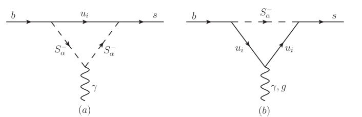
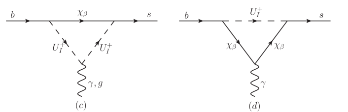
Figure 1: The Feynman diagrams contributing to $\bar{B}\rightarrow X_{s}\gamma$ from exotic fields in the $\mu\nu$SSM, compared with the SM.

Compared with the SM, the Feynman diagrams contributing to the process $\bar{B}\rightarrow X_{s}\gamma$ from exotic fields in the $\mu\nu$SSM are drawn in Fig. 1, where $S_{\alpha}^{-}$ ($\alpha=2,\ldots,8$) denote charged scalars, $U_{I}^{+}$ ($I=1,\ldots,6$) denote up-type squarks, $u_{i}$ ($i=1,2,3$) denote three generation of up-type quarks and $\chi_{\beta}$ ($\beta=1,\ldots,5$) denote charged fermions.

We could write the Wilson coefficients of the process $b\rightarrow s\gamma$ from the Feynman diagrams in Fig. 1 at the electroweak scale $\mu_{EW}$ as follow:

$$C_{7}^{NP}(\mu_{EW})=C_{7\gamma}^{NP}(\mu_{EW})+\widetilde{C}_{7\gamma}^{NP}(\mu_{EW}),$$ (13)

where the new physics contributions read

$$\widetilde{C}_{7\gamma}^{NP}(\mu_{EW})=\widetilde{C}_{7\gamma a}^{NP}(\mu_{EW})+\widetilde{C}_{7\gamma b}^{NP}(\mu_{EW})+\widetilde{C}_{7\gamma c}^{NP}(\mu_{EW})+\widetilde{C}_{7\gamma d}^{NP}(\mu_{EW}),$$ (14)

$$\widetilde{C}_{7\gamma a}^{NP}(\mu_{EW})=\sum\limits_{u_{i},S_{\alpha}^{-}}\frac{s_{{}_{W}}^{2}}{2e^{2}{V_{ts}^{\ast}V_{tb}}}\Big{\{}\frac{1}{2}C_{R}^{S_{\alpha}^{-}{\bar{s}}u_{i}}C_{R}^{S_{\alpha}^{-}{\bar{b}}u_{i}\ast}\Big{[}-{I_{3}}(x_{{u_{i}}},{x_{{S_{\alpha}^{-}}}})+{I_{4}}(x_{{u_{i}}},{x_{{S_{\alpha}^{-}}}})\Big{]}$$

$$\qquad\qquad\qquad\>+\frac{m_{u_{i}}}{m_{b}}C_{L}^{S_{\alpha}^{-}{\bar{s}}u_{i}}C_{R}^{S_{\alpha}^{-}{\bar{b}}u_{i}\ast}\Big{[}-{I_{1}}(x_{{u_{i}}},{x_{{S_{\alpha}^{-}}}})+{I_{3}}(x_{{u_{i}}},{x_{{S_{\alpha}^{-}}}})\Big{]}\Big{\}},$$ (15)

$$\widetilde{C}_{7\gamma b}^{NP}(\mu_{EW})=\sum\limits_{u_{i},S_{\alpha}^{-}}\frac{s_{{}_{W}}^{2}}{3e^{2}{V_{ts}^{\ast}V_{tb}}}\Big{\{}\frac{1}{2}C_{R}^{S_{\alpha}^{-}{\bar{s}}u_{i}}C_{R}^{S_{\alpha}^{-}{\bar{b}}u_{i}\ast}\Big{[}-{I_{1}}(x_{{u_{i}}},{x_{{S_{\alpha}^{-}}}})+2{I_{3}}(x_{{u_{i}}},{x_{{S_{\alpha}^{-}}}})$$

$$\qquad\qquad\qquad\>-{I_{4}}(x_{{u_{i}}},{x_{{S_{\alpha}^{-}}}})\Big{]}+\frac{m_{u_{i}}}{m_{b}}C_{L}^{S_{\alpha}^{-}{\bar{s}}u_{i}}C_{R}^{S_{\alpha}^{-}{\bar{b}}u_{i}\ast}\Big{[}{I_{1}}(x_{{u_{i}}},{x_{{S_{\alpha}^{-}}}})-{I_{2}}(x_{{u_{i}}},{x_{{S_{\alpha}^{-}}}})$$

$$\qquad\qquad\qquad\>-{I_{3}}(x_{{u_{i}}},{x_{{S_{\alpha}^{-}}}})\Big{]}\Big{\}},$$ (16)

$$\widetilde{C}_{7\gamma c}^{NP}(\mu_{EW})=\sum\limits_{\chi_{\beta},U_{I}^{+}}\frac{s_{{}_{W}}^{2}}{3e^{2}{V_{ts}^{\ast}V_{tb}}}\Big{\{}\frac{1}{2}C_{R}^{U_{I}^{+}{\bar{s}}\chi_{\beta}}C_{R}^{U_{I}^{+}{\bar{b}}\chi_{\beta}\ast}\Big{[}{I_{3}}({x_{{\chi_{\beta}}}},{x_{{U_{I}^{+}}}})-{I_{4}}({x_{{\chi_{\beta}}}},{x_{{U_{I}^{+}}}})\Big{]}$$

$$\qquad\qquad\qquad\>+\frac{m_{\chi_{\beta}}}{m_{b}}C_{L}^{U_{I}^{+}{\bar{s}}\chi_{\beta}}C_{R}^{U_{I}^{+}{\bar{b}}\chi_{\beta}\ast}\Big{[}{I_{1}}({x_{{\chi_{\beta}}}},{x_{{U_{I}^{+}}}})-{I_{3}}({x_{{\chi_{\beta}}}},{x_{{U_{I}^{+}}}})\Big{]}\Big{\}},$$ (17)

$$\widetilde{C}_{7\gamma d}^{NP}(\mu_{EW})=\sum\limits_{\chi_{\beta},U_{I}^{+}}\frac{s_{{}_{W}}^{2}}{2e^{2}{V_{ts}^{\ast}V_{tb}}}\Big{\{}\frac{1}{2}C_{R}^{U_{I}^{+}{\bar{s}}\chi_{\beta}}C_{R}^{U_{I}^{+}{\bar{b}}\chi_{\beta}\ast}\Big{[}-{I_{1}}({x_{{\chi_{\beta}}}},{x_{{U_{I}^{+}}}})+2{I_{3}}({x_{{\chi_{\beta}}}},{x_{{U_{I}^{+}}}})$$

$$\qquad\qquad\qquad\>-{I_{4}}({x_{{\chi_{\beta}}}},{x_{{U_{I}^{+}}}})\Big{]}+\frac{m_{\chi_{\beta}}}{m_{b}}C_{L}^{U_{I}^{+}{\bar{s}}\chi_{\beta}}C_{R}^{U_{I}^{+}{\bar{b}}\chi_{\beta}\ast}\Big{[}{I_{1}}({x_{{\chi_{\beta}}}},{x_{{U_{I}^{+}}}})-{I_{2}}({x_{{\chi_{\beta}}}},{x_{{U_{I}^{+}}}})$$

$$\qquad\qquad\qquad\>-{I_{3}}({x_{{\chi_{\beta}}}},{x_{{U_{I}^{+}}}})\Big{]}\Big{\}},$$ (18)

$$C_{7\gamma}^{NP}(\mu_{EW})=\left.\widetilde{C}_{7\gamma}^{NP}(\mu_{EW})\right|{{}_{L\leftrightarrow R}}.$$ (19)

Here the concrete expressions for coupling coefficients $C_{L,R}$ and form factors $I_{i}$ ($i=1,\ldots,4$) can be found in Appendixes A–B. Additionally, $x={m^{2}}/{m_{W}^{2}}$, where $m$ is the mass for the corresponding particle and $m_{W}$ is the mass for the $W$-boson.

The Feynman diagrams of the process $b\rightarrow sg$ from exotic fields in the $\mu\nu$SSM compared with the SM are shown in Fig. 1(b) and Fig. 1(c). Similarly, the Wilson coefficients of the process $b\rightarrow sg$ at electroweak scale are

$$C_{8}^{NP}(\mu_{EW})=C_{8g}^{NP}(\mu_{EW})+\widetilde{C}_{8g}^{NP}(\mu_{EW}),$$ (20)

$$\widetilde{C}_{8g}^{NP}(\mu_{EW})=\Big{[}\widetilde{C}_{7\gamma b}^{NP}(\mu_{EW})+\widetilde{C}_{7\gamma c}^{NP}(\mu_{EW})\Big{]}/{Q_{u}},$$ (21)

$$C_{8g}^{NP}(\mu_{EW})=\left.\widetilde{C}_{8g}^{NP}(\mu_{EW})\right|{{}_{L\leftrightarrow R}},$$ (22)

where $Q_{u}=2/3$.

In the $\mu\nu{\rm SSM}$, the expression for the branching ratio of $\bar{B}\rightarrow X_{s}\gamma$ is given as follow

$${\rm{Br}}(\bar{B}\rightarrow X_{s}\gamma)=R\Big{(}|C_{7\gamma}(\mu_{b})|^{2}+N(E_{\gamma})\Big{)}\;,$$ (23)

where the overall factor $R=2.47\times 10^{-3}$, and the nonperturbative contribution $N(E_{\gamma})=(3.6\pm 0.6)\times 10^{-3}$ ref13 . $C_{7\gamma}(\mu_{b})$ is defined by

$$C_{7\gamma}(\mu_{b})=C_{7\gamma}^{SM}(\mu_{b})+C_{7}^{NP}(\mu_{b}).$$ (24)

where we choose the hadron scale $\mu_{b}=2.5$ GeV and use the SM contribution at NNLO level $C_{7\gamma}^{SM}(\mu_{b})=-0.3523$ ref13 ; ref14 ; ref16 ; ref17-Czakon . The Wilson coefficients for new physics at the bottom quark scale can be written as ref19 ; refGao

$$C_{7}^{NP}(\mu_{b})\approx 0.5696C_{7}^{NP}(\mu_{EW})+0.1107C_{8}^{NP}(\mu_{EW}).$$ (25)

IV Numerical analysis

There are many free parameters in the SUSY extensions of the SM. In order to obtain a more transparent numerical results, we adopt the minimal flavor violating (MFV) assumption for some parameters in the $\mu\nu{\rm SSM}$, which assumes

$$\lambda_{i}=\lambda,\qquad{\kappa_{ijk}}=\kappa{\delta_{ij}}{\delta_{jk}},\quad{({A_{\kappa}}\kappa)_{ijk}}={A_{\kappa}}\kappa{\delta_{ij}}{\delta_{jk}},$$

$${({A_{\lambda}}\lambda)}_{i}={A_{\lambda}}\lambda,\quad{Y_{{\nu_{ij}}}}={Y_{{\nu_{i}}}}{\delta_{ij}},\qquad{Y_{{e_{ij}}}}={Y_{{e_{i}}}}{\delta_{ij}},$$

$$\upsilon_{\nu_{i}^{c}}=\upsilon_{\nu^{c}},\quad(A_{\nu}Y_{\nu})_{ij}={a_{{\nu_{i}}}}{\delta_{ij}},\quad{({A_{e}}{Y_{e}})_{ij}}={A_{e}}{Y_{{e_{i}}}}{\delta_{ij}},$$

$$m_{{{\tilde{L}}_{ij}}}^{2}=m_{\tilde{L}}^{2}{\delta_{ij}},\quad m_{\tilde{\nu}_{ij}^{c}}^{2}=m_{{{\tilde{\nu}_{i}}^{c}}}^{2}{\delta_{ij}},\quad m_{\tilde{e}_{ij}^{c}}^{2}=m_{{{\tilde{e}}^{c}}}^{2}{\delta_{ij}},$$

$$m_{\tilde{Q}_{ij}}^{2}=m_{{{\tilde{Q}}_{i}}}^{2}{\delta_{ij}},\quad m_{\tilde{u}_{ij}^{c}}^{2}=m_{{{{\tilde{u}}_{i}}^{c}}}^{2}{\delta_{ij}},\quad m_{\tilde{d}_{ij}^{c}}^{2}=m_{{{{\tilde{d}}_{i}}^{c}}}^{2}{\delta_{ij}},$$ (26)

and one can assume

$$(A_{u}Y_{u})_{ij}={A_{u_{i}}}{Y_{{u_{ij}}}},\quad{Y_{{u_{ij}}}}={Y_{{u_{i}}}}{V_{L_{ij}}^{u}},$$

$$(A_{d}Y_{d})_{ij}={A_{d_{i}}}{Y_{{d_{ij}}}},\quad{Y_{{d_{ij}}}}={Y_{{d_{i}}}}{V_{L_{ij}}^{d}},$$ (27)

where $V=V_{L}^{u}V_{L}^{d{\dagger}}$ denotes the CKM matrix ref23 . Restrained by the quark and lepton masses, we could have

$${Y_{{u_{i}}}}\simeq\frac{{{m_{{u_{i}}}}}}{{{\upsilon_{u}}}},\qquad{Y_{{d_{i}}}}\simeq\frac{{{m_{{d_{i}}}}}}{{{\upsilon_{d}}}},\qquad{Y_{{e_{i}}}}=\frac{{{m_{{l_{i}}}}}}{{{\upsilon_{d}}}},$$ (28)

where $m_{u_{i}}$, $m_{d_{i}}$ and $m_{l_{i}}$ are the up-quark, down-quark and charged lepton masses, respectively, and we choose the values from Ref. ref23 .

At the EW scale, the soft masses $m_{\tilde{H}_{d}}^{2}$, $m_{\tilde{H}_{u}}^{2}$ and $m_{\tilde{\nu}_{i}^{c}}^{2}$ can be derived from the minimization conditions of the tree-level neutral scalar potential, which are given in Refs. ref3 ; ref-zhang . Ignoring the terms of the second order in $Y_{\nu}$ and assuming $(\upsilon_{\nu_{i}}^{2}+\upsilon_{d}^{2}-\upsilon_{u}^{2})\approx(\upsilon_{d}^{2}-\upsilon_{u}^{2})$, one can solve the minimization conditions of the tree-level neutral scalar potential with respect to $\upsilon_{\nu_{i}}\>(i=1,2,3)$ as ref26

$$\upsilon_{\nu_{i}}=\frac{\lambda\upsilon_{d}(\upsilon_{u}^{2}+\upsilon_{\nu^{c}}^{2})-\kappa\upsilon_{u}\upsilon_{\nu^{c}}^{2}}{m_{\tilde{L}}^{2}+{G^{2}\over 4}(\upsilon_{d}^{2}-\upsilon_{u}^{2})}Y_{\nu_{i}}-\frac{\upsilon_{u}\upsilon_{\nu^{c}}}{m_{\tilde{L}}^{2}+{G^{2}\over 4}(\upsilon_{d}^{2}-\upsilon_{u}^{2})}a_{\nu_{i}},$$ (29)

where $G^{2}=g_{1}^{2}+g_{2}^{2}$ and $g_{1}c_{{}_{W}}=g_{2}s_{{}_{W}}=e$.

In the $\mu\nu{\rm SSM}$, the sneutrino sector may appear the tachyons. The masses squared of the tachyons are negative. So, we need analyse the masses of the sneutrinos. The masses of left-handed sneutrinos are basically determined by $m_{\tilde{L}}$, and the three right-handed sneutrinos are essentially degenerated. The CP-even and CP-odd right-handed sneutrino masses squared can be approximately written as ref-zhang1

$$m_{S_{5+i}}^{2}\approx(A_{\kappa}+4\kappa\upsilon_{\nu^{c}})\kappa\upsilon_{\nu^{c}}+A_{\lambda}\lambda\upsilon_{d}\upsilon_{u}/\upsilon_{\nu^{c}}-2\lambda^{2}(\upsilon_{d}^{2}+\upsilon_{u}^{2}),$$ (30)

$$m_{P_{5+i}}^{2}\approx-3A_{\kappa}\kappa\upsilon_{\nu^{c}}+(A_{\lambda}/\upsilon_{\nu^{c}}+4\kappa)\lambda\upsilon_{d}\upsilon_{u}-2\lambda^{2}(\upsilon_{d}^{2}+\upsilon_{u}^{2}).$$ (31)

Here, the main contribution for the mass squared is the first term as $\kappa$ is large, in the limit of $\upsilon_{\nu^{c}}\gg\upsilon_{u,d}$. Therefore, we could use the approximate relation

$$-4\kappa\upsilon_{\nu^{c}}\lesssim A_{\kappa}\lesssim 0,$$ (32)

to avoid the tachyons.

Before calculation, the constraints on the parameters of the $\mu\nu{\rm SSM}$ from neutrino experiments should be considered at first. Three flavor neutrinos $\nu_{e,\mu,\tau}$ could mix into three massive neutrinos $\nu_{1,2,3}$ during their flight, and the mixings are described by the Pontecorvo-Maki-Nakagawa-Sakata unitary matrix $U_{{}_{PMNS}}$ ref20 ; ref21 . The experimental observations of the parameters in $U_{{}_{PMNS}}$ for the normal mass hierarchy show that ref22

$$\sin^{2}\theta_{12}=0.302_{-0.012}^{+0.013},\qquad\Delta m_{21}^{2}=7.50_{-0.19}^{+0.18}\times 10^{-5}{\rm eV}^{2},$$

$$\sin^{2}\theta_{23}=0.413_{-0.025}^{+0.037},\qquad\Delta m_{31}^{2}=2.473_{-0.067}^{+0.070}\times 10^{-3}{\rm eV}^{2},$$

$$\sin^{2}\theta_{13}=0.0227_{-0.0024}^{+0.0023}.$$ (33)

In the $\mu\nu{\rm SSM}$, the three neutrino masses are obtained through a TeV scale seesaw mechanism ref2 ; ref26 ; ref27 ; ref28 ; ref29 ; refneu ; refneu1 . Assumed that the charged lepton mass matrix in the flavor basis is in the diagonal form, we parameterize the unitary matrix which diagonalizes the effective light neutrino mass matrix $m_{eff}$ (see Ref. ref-zhang ) as ref30 ; ref31

$${U_{\nu}}= \left({\begin{array}[]{*{20}{c}}{{c_{12}}{c_{13}}}&{{s_{12}}{c_{13}}}&{{s_{13}}{e^{-i\delta}}}\\ {-{s_{12}}{c_{23}}-{c_{12}}{s_{23}}{s_{13}}{e^{i\delta}}}&{{c_{12}}{c_{23}}-{s_{12}}{s_{23}}{s_{13}}{e^{i\delta}}}&{{s_{23}}{c_{13}}}\\ {{s_{12}}{s_{23}}-{c_{12}}{c_{23}}{s_{13}}{e^{i\delta}}}&{-{c_{12}}{s_{23}}-{s_{12}}{c_{23}}{s_{13}}{e^{i\delta}}}&{{c_{23}}{c_{13}}}\\ \end{array}}\right)$$ (38)

$$\times\>diag(1,{e^{i\frac{{{\alpha_{21}}}}{2}}},{e^{i\frac{{{\alpha_{31}}}}{2}}})\>,$$

where ${c_{{}_{ij}}}=\cos{\theta_{ij}}$, ${s_{{}_{ij}}}=\sin{\theta_{ij}}$. In our calculation, the values of $\theta_{ij}$ are obtained from the experimental data in Eq. (33), and all CP violating phases $\delta$, $\alpha_{21}$ and $\alpha_{31}$ are set to zero. $U_{\nu}$ diagonalizes $m_{eff}$ in the following way:

$$U_{\nu}^{T}m_{eff}^{T}{m_{eff}}{U_{\nu}}=diag({m_{\nu_{1}}^{2}},{m_{\nu_{2}}^{2}},{m_{\nu_{3}}^{2}}).$$ (39)

For the neutrino mass spectrum, we assume it to be normal hierarchical, i.e., ${m_{\nu_{1}}}{\rm{<}}{m_{\nu_{2}}}{\rm{<}}{m_{\nu_{3}}}$, and we choose the neutrino mass $m_{\nu_{1}}=10^{-2}\>{\rm{eV}}$ as input in our numerical analysis, considered that the tiny neutrino masses basically don’t affect ${\rm{Br}}(\bar{B}\rightarrow X_{s}\gamma)$ in the following and limited on neutrino masses from neutrinoless double-$\beta$ decay neu-m-limit and cosmology neu-m-limit1 . The other two neutrino masses $m_{\nu_{2,3}}$ can be obtained through the experimental data on the differences of neutrino mass squared in Eq. (33). Then, we can numerically derive $Y_{\nu_{i}}\sim\mathcal{O}(10^{-7})$ and $a_{\nu_{i}}\sim\mathcal{O}(-10^{-4}{\rm{GeV}})$ from Eq. (39). Accordingly, $\upsilon_{\nu_{i}}\sim\mathcal{O}(10^{-4}{\rm{GeV}})$ through Eq. (29). Due to $\upsilon_{\nu_{i}}\ll\upsilon_{u,d}$, we can have

$$\tan\beta\simeq\frac{\upsilon_{u}}{\upsilon_{d}}.$$ (40)

Recently, a neutral Higgs with mass around $125\;{\rm GeV}$ reported by ATLAS ATLAS and CMS CMS also contributes a strict constraint on relevant parameter space of the model. The global fit to the ATLAS and CMS Higgs data gives mh-AC :

$$m_{{h}}=125.7\pm 0.4\;{\rm GeV}.$$ (41)

Due to the introduction of some new couplings in the superpotential, the SM-like Higgs mass in the $\mu\nu$SSM gets additional contribution at tree-level ref3 . For moderate $\tan\beta$ and large mass of the pseudoscalar $M_{A}$, the SM-like Higgs mass in the $\mu\nu{\rm SSM}$ is approximately given by

$$m_{h}^{2}\simeq m_{Z}^{2}\cos^{2}2\beta+\frac{6\lambda^{2}s_{{}_{W}}^{2}c_{{}_{W}}^{2}}{e^{2}}m_{Z}^{2}\sin^{2}2\beta+\bigtriangleup m_{h}^{2}.$$ (42)

Compared with the MSSM, the $\mu\nu{\rm SSM}$ gets an additional term $\frac{6\lambda^{2}s_{{}_{W}}^{2}c_{{}_{W}}^{2}}{e^{2}}m_{Z}^{2}\sin^{2}2\beta$. Therefore, the SM-like Higgs in the $\mu\nu{\rm SSM}$ can easily account for the mass around $125\,{\rm GeV}$, especially for small $\tan\beta$. Including two-loop leading-log effects, the main radiative corrections can be given by ref-mh-rad1 ; ref-mh-rad2 ; ref-mh-rad3

$$\bigtriangleup m_{h}^{2}=\frac{3m_{t}^{4}}{4\pi^{2}\upsilon^{2}}\Big{[}(t+\frac{1}{2}{\tilde{X}_{t}})+\frac{1}{16\pi^{2}}(\frac{3m_{t}^{2}}{2\upsilon^{2}}-32\pi\alpha_{3})(t^{2}+{\tilde{X}_{t}}t)\Big{]},$$ (43)

with

$$t=\log\frac{M_{S}^{2}}{m_{t}^{2}},\qquad{\tilde{X}_{t}}=\frac{2\tilde{A}_{t}^{2}}{M_{S}^{2}}\Big{(}1-\frac{\tilde{A}_{t}^{2}}{12M_{S}^{2}}\Big{)},$$ (44)

where $\upsilon=174$ GeV, $M_{S}=\sqrt{m_{{\tilde{t}}_{1}}m_{{\tilde{t}}_{2}}}$ with $m_{{\tilde{t}}_{1,2}}$ being the stop masses, $\alpha_{3}$ is the strong coupling constant, $\tilde{A}_{t}=A_{t}-\mu\cot\beta$ with $A_{t}$ denoting the trilinear Higgs-stop coupling and $\mu=3\lambda\upsilon_{\nu^{c}}$ being the Higgsino mass parameter.

Through the analysis of the parameter space in Ref. ref3 , we could choose the reasonable values for some parameters as $\kappa=0.4$, $\lambda=0.2$, $\upsilon_{\nu^{c}}=1\;{\rm TeV}$ and $m_{\tilde{L}}=m_{{\tilde{e}}^{c}}={A_{e}}=1\;{\rm TeV}$ for simplicity in the following numerical calculation. Through Eq. (32), we could choose ${A_{\kappa}}=-300\;{\rm GeV}$ to avoid the tachyons. For the Majorana masses of the gauginos, we will imply the approximate GUT relation $M_{1}=\frac{\alpha_{1}^{2}}{\alpha_{2}^{2}}M_{2}\approx 0.5M_{2}$ and $M_{3}=\frac{\alpha_{3}^{2}}{\alpha_{2}^{2}}M_{2}\approx 2.7M_{2}$. The gluino mass, $m_{{\tilde{g}}}\approx M_{3}$, is larger than about $1.2$ TeV from the ATLAS and CMS experimental data ATLAS-sg1 ; ATLAS-sg2 ; CMS-sg1 ; CMS-sg2 . So, we conservatively choose $M_{2}=1\;{\rm TeV}$. The first two generations of squarks are strongly constrained by direct searches at the LHC ATLAS-sq1 ; CMS-sq1 . Therefore, we take $m_{{\tilde{Q}}_{1,2}}=m_{{\tilde{u}}^{c}_{1,2}}=m_{{\tilde{d}}^{c}_{1,2}}=2\;{\rm TeV}$. The third generation squark masses are not constrained by the LHC as strongly as the first two generations, and affect the SM-like Higgs mass. So, we could adopt $m_{{\tilde{Q}}_{3}}=m_{{\tilde{u}}^{c}_{3}}=m_{{\tilde{d}}^{c}_{3}}=1\;{\rm TeV}$. When the masses of squarks are TeV scale, the contributions to ${\rm{Br}}(\bar{B}\rightarrow X_{s}\gamma)$ of squarks become small, so we could reasonably use the above choice in the following calculation. For simplicity, we also choose $A_{d_{1,2,3}}=A_{u_{1,2}}=1\;{\rm TeV}$. As a key parameter, $A_{u_{3}}=A_{t}$ affects the following numerical calculation. In the limit of $\upsilon_{\nu^{c}}\gg\upsilon_{u,d}$ ref-limit-MH , the charged Higgs mass squared $M_{H^{\pm}}^{2}$ in the $\mu\nu$SSM can be formulated as

$$M_{H^{\pm}}^{2}\simeq M_{A}^{2}+(1-\frac{6s_{{}_{W}}^{2}\lambda^{2}}{e^{2}})m_{W}^{2},$$ (45)

with the neutral pseudoscalar mass squared

$$M_{A}^{2}\simeq\frac{6\lambda\upsilon_{\nu^{c}}(A_{\lambda}+\kappa\upsilon_{\nu^{c}})}{\sin 2\beta}.$$ (46)

Considered that $M_{H^{\pm}}$ also is a key parameter which affects the numerical results, we could take $M_{H^{\pm}}$ as input to constrain the parameter $A_{\lambda}$.

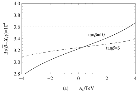
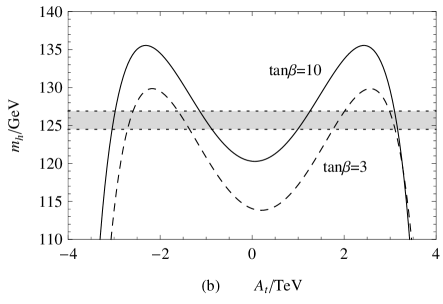
Figure 2: (a) ${\rm{Br}}(\bar{B}\rightarrow X_{s}\gamma)$ versus $A_{t}$ for $\tan\beta=3$ (dashed line) and $\tan\beta=10$ (solid line), when $M_{H^{\pm}}=1.5$ TeV. The dotted lines represent the experimental $1\sigma$ bounds. (b) The SM-like Higgs mass $m_{h}$ versus $A_{t}$ for $\tan\beta=3$ (dashed line) and $\tan\beta=10$ (solid line), where the gray area denotes the experimental $3\sigma$ interval.

Similarly to the MSSM and NMSSM B-NMSSM , the new physics contributions to the branching ratio of $\bar{B}\rightarrow X_{s}\gamma$ in the $\mu\nu{\rm SSM}$ depend essentially on the charged Higgs mass $M_{H^{\pm}}$, $\tan\beta$ and $A_{t}$. When $M_{H^{\pm}}=1.5$ TeV, we plot ${\rm{Br}}(\bar{B}\rightarrow X_{s}\gamma)$ versus $A_{t}$ in Fig. 2(a), for $\tan\beta=3$ (dashed line) and $\tan\beta=10$ (solid line). The dotted lines represent the experimental $1\sigma$ bounds. The numerical results show that ${\rm{Br}}(\bar{B}\rightarrow X_{s}\gamma)$ increases with increasing of $A_{t}$, and the slope of evolution for ${\rm{Br}}(\bar{B}\rightarrow X_{s}\gamma)$ is big as $\tan\beta$ is large. In Fig. 2(a), ${\rm{Br}}(\bar{B}\rightarrow X_{s}\gamma)$ will be easily below the experimental $1\sigma$ lower bound, when $A_{t}$ is negative. For positive $A_{t}$, ${\rm{Br}}(\bar{B}\rightarrow X_{s}\gamma)$ still can exceed the experimental $1\sigma$ upper bound, as $\tan\beta$ is large enough. So the new physics can give the considerable contributions to ${\rm{Br}}(\bar{B}\rightarrow X_{s}\gamma)$ for large $\tan\beta$ and $A_{t}$.

We also need consider the constraint of the SM-like Higgs mass. So in Fig. 2(b), we plot the SM-like Higgs mass $m_{h}$ versus $A_{t}$ for $\tan\beta=3$ (dashed line) and $\tan\beta=10$ (solid line), where the gray area denotes the experimental $3\sigma$ interval. When $\tan\beta=3$, we require that $A_{t}$ is about $-2.65$, $-1.5$, $1.9$ or $3.05$ TeV to keep the SM-like Higgs mass around 125 GeV. For $\tan\beta=10$, we need $A_{t}$ to be about $-3.0$, $-1.0$, $1.1$ or $3.13$ TeV, keeping the SM-like Higgs mass around 125 GeV.

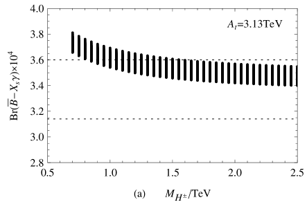
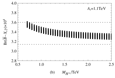
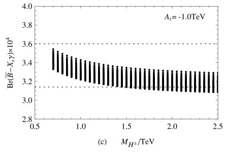
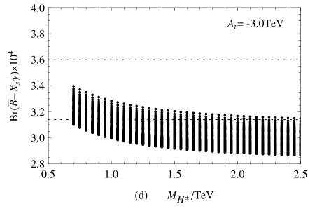
Figure 3: ${\rm{Br}}(\bar{B}\rightarrow X_{s}\gamma)$ versus $M_{H^{\pm}}$ for (a) $A_{t}=3.13$ TeV, (b) $A_{t}=1.1$ TeV, (c) $A_{t}=-1.0$ TeV and (d) $A_{t}=-3.0$ TeV, respectively, when $\tan\beta=10$. Here, we scan over the parameters $\upsilon_{\nu^{c}}$ and $M_{2}$ between 0.5 TeV and 1.5 TeV, which step is 0.05 TeV. The horizontal dotted lines represent the experimental $1\sigma$ bounds.

In large $M_{A}$ limit, the charged Higgs mass, $M_{H^{\pm}}\sim M_{A}\sim M_{H}$, doesn’t affect the SM-like Higgs mass. So, we could choose $A_{t}=-3.0$, $-1.0$, $1.1$ or $3.13$ TeV, for $\tan\beta=10$, to keep the SM-like Higgs mass around 125 GeV. Then, we draw ${\rm{Br}}(\bar{B}\rightarrow X_{s}\gamma)$ versus $M_{H^{\pm}}$ in Fig. 3, for (a) $A_{t}=3.13$ TeV, (b) $A_{t}=1.1$ TeV, (c) $A_{t}=-1.0$ TeV and (d) $A_{t}=-3.0$ TeV, respectively, when $\tan\beta=10$. The horizontal dotted lines represent the experimental $1\sigma$ bounds. Here, we scan over the parameters $\upsilon_{\nu^{c}}$ and $M_{2}$ between 0.5 TeV and 1.5 TeV, which step is 0.05 TeV. For some $M_{H^{\pm}}$ and $A_{t}$, when $\upsilon_{\nu^{c}}$ and $M_{2}$ are small, ${\rm{Br}}(\bar{B}\rightarrow X_{s}\gamma)$ become large. Because the chargino masses are dependent on $\upsilon_{\nu^{c}}$ and $M_{2}$, which can give contributions to ${\rm{Br}}(\bar{B}\rightarrow X_{s}\gamma)$ through chargino-squark loop diagrams in Fig. 1 (c) and (d). Due to constrain the heavy doublet-like Higgs mass $M_{H}\geq 642$ GeV CMS-600 ; ATLAS-642 , we take the charged Higgs mass $M_{H^{\pm}}\gtrsim 700$ GeV. The numerical results show that ${\rm{Br}}(\bar{B}\rightarrow X_{s}\gamma)$ decreases along with increasing of $M_{H^{\pm}}$, because the contributions from charged Higgs diagrams decay like $1/M_{H^{\pm}}^{4}$ B-NMSSM . For small $M_{H^{\pm}}$, the new physics could contribute with large corrections to the branching ratio of $\bar{B}\rightarrow X_{s}\gamma$. In Fig. 3, ${\rm{Br}}(\bar{B}\rightarrow X_{s}\gamma)$ can exceed the experimental $1\sigma$ upper bound for small $M_{H^{\pm}}$, when $A_{t}=3.13$ TeV. In addition, ${\rm{Br}}(\bar{B}\rightarrow X_{s}\gamma)$ can be easily below the experimental $1\sigma$ lower bound for $A_{t}=-3.0$ TeV, which is excluded by the experimental value at $1\sigma$ level.

V Conclusion

The flavour changing neutral current process $\bar{B}\rightarrow X_{s}\gamma$ offers high sensitivity to new physics. In this work, we investigate the branching ratio of the rare decay $\bar{B}\rightarrow X_{s}\gamma$ in the framework of $\mu\nu$SSM under a minimal flavor violating assumption. Similarly to the MSSM and NMSSM, the new physics contributions to ${\rm{Br}}(\bar{B}\rightarrow X_{s}\gamma)$ in the $\mu\nu{\rm SSM}$ depend essentially on the charged Higgs mass $M_{H^{\pm}}$, $\tan\beta$ and $A_{t}$, because the mixings between charginos and charged leptons in the mass matrix of the $\mu\nu$SSM are suppressed, as well as those between charged Higgses and charged sleptons. Under the constraint of the SM-like Higgs with mass around 125 GeV, the numerical results show that the new physics can fit the experimental data for the rare decay $\bar{B}\rightarrow X_{s}\gamma$ and further constrain the parameter space. Besides $\bar{B}\rightarrow X_{s}\gamma$, other $b\rightarrow s$ transitions e.g. $\Delta M_{s}$, $S_{J/\psi\phi}$, $B_{s}\rightarrow\mu^{+}\mu^{-}$ also may give some constraints on relevant parameter space in this model, we will investigate this elsewhere in detail.

Appendix A The interaction Lagrangian

In the $\mu\nu$SSM, The corresponding interaction Lagrangian of the $\bar{B}\rightarrow X_{s}\gamma$ process is written as

$$\mathcal{L}_{int}=\Big{[}S_{\alpha}^{-}\bar{d}_{i}(C_{L}^{S_{\alpha}^{-}\bar{d}_{i}u_{j}}{P_{L}}+C_{R}^{S_{\alpha}^{-}\bar{d}_{i}u_{j}}{P_{R}})u_{j}$$

$$\hskip 42.67912pt+\>U_{I}^{+}\bar{d}_{i}(C_{L}^{U_{I}^{+}\bar{d}_{i}{\chi_{\alpha}}}{P_{L}}+C_{R}^{U_{I}^{+}\bar{d}_{i}{\chi_{\alpha}}}{P_{R}})\chi_{\alpha}\Big{]}+{\rm{H.c.}},$$ (47)

with $P_{L,R}={(1\mp{\gamma_{5}})}/2$, and the coefficients are

$$C_{L}^{S_{\alpha}^{-}\bar{d}_{i}u_{j}}=Y_{d_{i}}R_{S^{\pm}}^{1\alpha}V_{ji}^{\ast},$$ (48)

$$C_{R}^{S_{\alpha}^{-}\bar{d}_{i}u_{j}}=Y_{u_{j}}R_{S^{\pm}}^{2\alpha}V_{ji}^{\ast},$$ (49)

$$C_{L}^{U_{I}^{+}\bar{d}_{i}{\chi_{\alpha}}}={Y_{d_{i}}}Z_{-}^{2\alpha}R_{u}^{jI}V_{ji}^{\ast},$$ (50)

$$C_{R}^{U_{I}^{+}\bar{d}_{i}{\chi_{\alpha}}}=\Big{[}-\frac{e}{s_{{}_{W}}}Z_{+}^{1\alpha\ast}R_{u}^{jI}+{Y_{u_{j}}}Z_{+}^{2\alpha\ast}R_{u}^{(3+j)I}\Big{]}V_{ji}^{\ast},$$ (51)

where $R_{S^{\pm}}$, $R_{u}$ and $Z_{\mp}$ can be found in Ref. ref-zhang , and $V_{ji}$ denote the quark mixing matrix elements.

Appendix B Form factors

Defining ${x_{i}}=\frac{{m_{i}^{2}}}{{m_{W}^{2}}}$, we can have the form factors:

$${I_{1}}(\textit{x}_{1},x_{2})=\frac{{1+\ln{x_{2}}}}{{({x_{2}}-{x_{1}})}}+\frac{{{x_{1}}\ln{x_{1}}}-{{x_{2}}\ln{x_{2}}}}{{{{({x_{2}}-{x_{1}})}^{2}}}},$$ (52)

$${I_{2}}(\textit{x}_{1},x_{2})=-\frac{{1+\ln{x_{1}}}}{{({x_{2}}-{x_{1}})}}-\frac{{{x_{1}}\ln{x_{1}}}-{{x_{2}}\ln{x_{2}}}}{{{{({x_{2}}-{x_{1}})}^{2}}}},$$ (53)

$${I_{3}}(\textit{x}_{1},x_{2})=\frac{1}{2}\Big{[}\frac{{3+2\ln{x_{2}}}}{{({x_{2}}-{x_{1}})}}-\frac{{2{x_{2}}+4{x_{2}}\ln{x_{2}}}}{{{{({x_{2}}-{x_{1}})}^{2}}}}-\frac{{2x_{1}^{2}\ln{x_{1}}}}{{{{({x_{2}}-{x_{1}})}^{3}}}}+\frac{{2x_{2}^{2}\ln{x_{2}}}}{{{{({x_{2}}-{x_{1}})}^{3}}}}\Big{]},$$ (54)

$${I_{4}}(\textit{x}_{1},x_{2})=\frac{1}{6}\Big{[}\frac{{11+6\ln{x_{2}}}}{{({x_{2}}-{x_{1}})}}-\frac{{15{x_{2}}+18{x_{2}}\ln{x_{2}}}}{{{{({x_{2}}-{x_{1}})}^{2}}}}+\frac{{6x_{2}^{2}+18x_{2}^{2}\ln{x_{2}}}}{{{{({x_{2}}-{x_{1}})}^{3}}}}$$

$$\hskip 68.28644pt+\>\frac{{6x_{1}^{3}\ln{x_{1}}}-{6x_{2}^{3}\ln{x_{2}}}}{{{{({x_{2}}-{x_{1}})}^{4}}}}\Big{]}.$$ (55)

References

(1) S. Chen, et al., CLEO Collaboration, Phys. Rev. Lett. 87 (2001) 251807.
(2) K. Abe, et al., BELLE Collaboration, Phys. Lett. B 511 (2001) 151.
(3) A. Limosani, et al., BELLE Collaboration, Phys. Rev. Lett. 103 (2009) 241801.
(4) J. P. Lees, et al., BABAR Collaboration, Phys. Rev. Lett. 109 (2012) 191801.
(5) J. P. Lees, et al., BABAR Collaboration, Phys. Rev. D 86 (2012) 112008.
(6) J. P. Lees, et al., BABAR Collaboration, Phys. Rev. D 86 (2012) 052012.
(7) B. Aubert, et al., BABAR Collaboration, Phys. Rev. D 77 (2008) 051103.
(8) S. Stone, PoS ICHEP 2012 (2013) 033.
(9) M. Misiak, et al., Phys. Rev. Lett. 98 (2007) 022002.
(10) M. Misiak, M. Steinhauser, Nucl. Phys. B 764 (2007) 62.
(11) K. Chetyrkin, M. Misiak, M. Munz, Phys. Lett. B 400 (1997) 206.
(12) C. Greub, T. Hurth, D. Wyler, Phys. Rev. D 54 (1996) 3350.
(13) K. Adel, Y.-P Yao, Phys. Rev. D 49 (1994) 4945.
(14) A. Ali, C. Greub, Phys. Lett. B 361 (1995) 146.
(15) D. E. López-Fogliani, C. Muñoz, Phys. Rev. Lett. 97 (2006) 041801.
(16) N. Escudero, D. E. López-Fogliani, C. Muñoz, R. Ruiz de Austri, JHEP 0812 (2008) 099.
(17) J. Fidalgo, D. E. López-Fogliani, C. Muñoz, R. Ruiz de Austri, JHEP 1110 (2011) 020.
(18) J. E. Kim, H. P. Nilles, Phys. Lett. B 138 (1984) 150.
(19) H. P. Nilles, Phys. Rept. 110 (1984) 1.
(20) H. E. Haber, G. L. Kane, Phys. Rept. 117 (1985) 75.