Steady entanglements in bosonic dissipative networks

Abstract

In this letter we propose a scheme for the preparation of steady entanglements in bosonic dissipative networks. We describe its implementation in a system of coupled cavities interacting with an engineered reservoir built up of three-level atoms. Emblematic bipartite ($Bell$ and $NOON$) and multipartite ($W$-class) states can be produced with high fidelity and purity.

The development of strategies to prepare nonclassical states of the radiation and the vibrational fields PNS and, in particular, to protect them against decoherence —by means of decoherence-free subspaces DFS , dynamical decoupling DD , and reservoir engineering PCZ ; RE — has long played a significant role in quantum optics. On the conceptual side, the need for these states stems from their use in the study of fundamental quantum processes, for instance to track decoherence Decoherence and the quantum-to-classical transition QC . At the practical level, mastery in handling these states is sought in the rapidly growing field of quantum information theory —which has recently mobilized practically all areas of low-energy physics— so as to implement the logic operations required for quantum computation and communication Livro .

The proposition of schemes that enable the generation of nonclassical equilibrium states has been one of the main tasks in the field of quantum information science. In this regard, the reservoir engineering technique proposed in 1996 PCZ and experimentally demonstrated four years latter in a trapped-ion system IT signalled an important step towards the implementation of quantum information processes Livro . Moreover, the protection of a particular state demands the (not always easy) engineering of a specific interaction which the system of interest is forced to perform with other, auxiliary, quantum systems. In the most important case of preparing and protecting entangled states, recent theoretical protocols, also based on engineering the decay process re , have all been shown possible with only dissipation as a resource. However, most of these theoretical schemes concentrate on the preparation of atomic maximally entangled states of two qubits 2atom , the $W$ state of three qubits 3atom or atomic multipartite entangled states Natom . Furthermore, we could mention schemes for preparing non-maximal steady entanglements of two or three oscillators coupled to a common reservoir 2harmonic , while, more recently, a proposal has been advanced to engineer a common squeezed reservoir for an ensemble of oscillators that has genuine multipartite entanglement Nharmonic .

In this Letter, based on our previous work FockEPL concerning a scheme to obtain Fock equilibrium states in a single cavity mode, we present a strategy to produce high-fidelity steady entanglements in coupled quantum harmonic oscillators (QHOs). Our protocol can be readily understood in terms of the map between the natural oscillators and the normal-mode basis, in which a prepared steady Fock state in a giving normal-mode oscillator must correspond to a steady entangled state in the natural basis. The engineered reservoir is built from a selective Jaynes-Cummings interaction WilsonJOPB , in accordance with the prescription in FockEPL , prompting the emergence of an engineered selective Liouvillian to govern the normal-mode dynamics, alongside the Liouvillian accounting for the natural loss mechanisms. We stress, from a practical perspective, that atomic reservoirs have for some time been used for the preparation of the cavity vacuum state RMP . Moreover, this has been theoretically explored, in close relation to the reservoir engineering technique PCZ , for the generation of an Einstein-Podolsky-Rosen steady state comprising two squeezed modes of a high-finesse cavity BR . We note that, the atomic reservoir can be implemented in other contexts of atom-field interaction, such as trapped ions Rafael and circuit QED Nori , where the required beam of atoms is simulated by a pulsed classical field. In trapped ions, the classical field is used intermittently to couple the vibrational mode with internal electronic states, while in circuit QED, it is used to bring a Cooper-pair box into resonance with the mode of a superconducting strip.

In our protocol, the steady state is driven by a sum of three engineered Lindbladians, two of which act upon selected subspaces of the normal mode space, one for photon emission and the other for photon absorption, within the corresponding selected subspaces. The third Lindbladian is associated with (non-selective) photon absorption by the normal mode, to counterbalance the inevitable emission to the natural (nonengineered) environment. The selective Lindbladians are built up from engineered selective Jaynes-Cummings (JC) Hamiltonians, while the nonselective Lindbladian follows from the usual JC interaction. We present here a brief review of the steps in the derivation of the master equation of a bosonic network, as developed in Temp . We note that a given topology of a network composed of $N$ QHOs is defined by the way the oscillators are coupled together, the set of coupling strengths $\{\lambda_{mn}\}$ and their natural frequencies $\{\omega_{m}\}$. Here we assume the general scenario, where each oscillator is coupled to its own reservoir, instead of the particular situation where the whole network is coupled to a common reservoir. From here on, setting the indices $m$ and $n$ to run from $1$ to $N$, the Hamiltonian $H=H_{S}+H_{R}+H_{I}$ modelling this network accounts for the $N$ coupled oscillators, given by ($\hbar=1$):

$$H_{s}=\sum_{m}\left[\omega_{m}a_{m}^{\dagger}a_{m}+\sum_{n(\neq m)}\lambda_{mn}(a_{m}^{\dagger}a_{n}+a_{m}a_{n}^{\dagger})\right],$$ (1)

where the $N$ distinct reservoirs, $H_{R}=\sum_{m}\sum_{k}\omega_{mk}b_{mk}^{\dagger}k_{mk}$, are each composed of an infinite set of $\{k\}$ modes, and the coupling between the QHOs and their respective reservoirs: $H_{I}=\sum_{m}\sum_{k}V_{mk}(b_{mk}^{\dagger}a_{m}+b_{mk}a_{m}^{\dagger})$. In the above, $a_{m}^{\dagger}$($a_{m}$) is the creation (annihilation) operator associated with the $mth$ network oscillator ($\omega_{m}$), which is coupled to the $nth$ oscillator with strength $\lambda_{mn}$ and to the $mth$ reservoir with strength $V_{mk}$. The $kth$ reservoir mode $\omega_{mk}$ is described by the creation (annihilation) operator $b_{mk}^{\dagger}$($b_{mk}$). To derive the master equation from Hamiltonian $H$, we first rewrite $H_{S}$ in a matrix form, $H_{s}=\sum_{m,n}a_{m}^{\dagger}\mathcal{H}_{mn}a_{m}$, the elements being given by $\mathcal{H}_{mn}=\omega_{m}\delta_{mn}+\lambda_{mn}(1-\delta_{mn}).$ The diagonalization of $\mathcal{H}$ is thus performed through the canonical transformation $A_{m}=\sum_{n}C_{mn}a_{n}$, where the coefficients of the $mth$ line of matrix $C$ define the eigenvectors associated with the eigenvalues $\overline{\omega}_{m}$ of $\mathcal{H}$. $C$ being an orthogonal matrix, $C^{T}$ $=C^{-1}$, the commutation relations $\left[A_{m,}A_{n}^{\dagger}\right]=\delta_{mn}$ and $\left[A_{m,}A_{n}\right]=0$ follow, enabling the Hamiltonian $H$ to be rewritten as $\ H=H_{0}+V$, where $H_{0}=\sum_{m}\left[\overline{\omega}_{m}A_{m}^{\dagger}A_{m}+\sum_{k}\omega_{mk}b_{mk}^{\dagger}k_{mk}\right]$ and $V=\sum_{m,n}\sum_{k}V_{mk}(b_{mk}^{\dagger}A_{n}+b_{mk}A_{n}^{\dagger})$. With the diagonalized Hamiltonian $H_{0}$, we are ready to introduce the interaction picture, defined by the transformation $U(t)=\exp(-\imath H_{0}t),$ in which $V_{I}(t)=\sum_{m,n}(\mathcal{O}_{mn}(t)A_{n}^{\dagger}+\mathcal{O}_{mn}^{\dagger}A_{n}),$ with the bath operator $\mathcal{O}_{mn}(t)=C_{nm}\sum_{k}V_{mk}\exp[-\imath(\omega_{mk}-\overline{\omega}_{m})t]b_{mk}.$ Assuming the interactions between the oscillators and the reservoirs to be weak enough, we perform a second-order perturbation approximation, followed by tracing out the reservoir degrees of freedom. We also assume a Markovian reservoir, where the time-dependent density operator of the network can be factorized from the reservoir: $\rho_{1\ldots N}(t)\otimes\rho_{R}(0).$

Next, we assume that the reservoir frequencies are sufficiently closely spaced to allow a continuum summation and, as usual, that the coupling strength $V_{m}(\overline{\omega})$ and the density of states $\sigma(\overline{\omega})$ of the $mth$ reservoir are slowly varying functions. Moreover, assuming Markovian white noise reservoirs, where the damping rates read $\gamma_{m}(\overline{\omega}_{k})=\gamma_{m\text{ }}$, the average excitation of the reservoir associated with the $mth$ oscillator  is $\left\langle b_{m}^{\dagger}(\overline{\omega}_{k})b_{m}(\overline{\omega}_{k})\right\rangle=\overline{n}_{m}(\overline{\omega}_{k})=\overline{n}_{m}$ and the cross-decay terms $\gamma_{mn\text{ }}$are null Temp , we obtain the normal mode master equation

$$\frac{d\rho}{dt}=-\imath[\overline{H},\rho]+\mathcal{L}\rho,$$ (2)

where $\overline{H}=\sum_{m}\overline{\omega}_{m}A_{m}^{\dagger}A_{m}$ and the Liouvillian

$$\mathcal{L}\rho =\mathop{\displaystyle\sum}_{m}\frac{\gamma_{m}}{2}(1+\overline{n}_{m})\left(2A_{m}\rho A_{m}^{\dagger}-\rho A_{m}^{\dagger}A_{m}-A_{m}^{\dagger}A_{m}\rho\right)$$ (3)

$$+\mathop{\displaystyle\sum}_{m}\frac{\gamma_{m}}{2}\overline{n}_{m}\left(2A_{m}^{\dagger}\rho A_{m}-\rho A_{m}A_{m}^{\dagger}-A_{m}A_{m}^{\dagger}\rho\right).$$ (4)

Our strategy to produce equilibrium entanglements in a bosonic dissipative network demands an engineered selective Liouvillian, to be added to the master equation (2), having the following structure:

$$\mathcal{L}_{eng}\rho =\mathop{\displaystyle\sum}_{m}\frac{\Gamma_{m\ell}}{2}\left(2A_{m\ell}\rho A_{m\ell}^{\dagger}-\rho A_{m\ell}^{\dagger}A_{m\ell}-A_{m\ell}^{\dagger}A_{m\ell}\rho\right)$$

$${\small+}\mathop{\displaystyle\sum}_{m}\frac{\Gamma_{m\ell^{\prime}}}{2}\left(2A_{m\ell^{\prime}}^{\dagger}\rho A_{m\ell^{\prime}}-\rho A_{m\ell^{\prime}}A_{m\ell^{\prime}}^{\dagger}-A_{m\ell^{\prime}}A_{m\ell^{\prime}}^{\dagger}\rho\right)$$

$${\small+}\mathop{\displaystyle\sum}_{m}\frac{\Gamma_{m}}{2}\left(2A_{m}\rho A_{A_{m}^{\dagger}}-\rho A_{m}^{\dagger}A_{m}-A_{m}^{\dagger}A_{m}\rho\right),$$ (5)

where $A_{m\ell}^{\dagger}=\left|\ell+1\right\rangle\left\langle\ell\right|$ $(A_{m\ell}=\left|\ell\right\rangle\left\langle\ell+1\right|)$ is a selective creation (annihilation) operator acting on the Fock subspace $\left\{\left|\ell\right\rangle,\left|\ell+1\right\rangle\right\}$ of the $mth$ normal mode. The engineered Liouvillians associated with the effective decay rates $\Gamma_{m\ell}$ and $\Gamma_{m\ell^{\prime}}$ account for selective emission and absorption terms, while the engineered Liouvillian associated with $\Gamma_{m}$ represents an additional cooling term. This latter Liouvillian must be taken into account, as will become clear later, only when preparing a required equilibrium state where at least one of the normal modes, the $n$th, is in the vacuum state. If the normal modes are not degenerate and the effective decay rates satisfy $\Gamma_{m\ell},\Gamma_{m\ell^{\prime}},\Gamma_{n\neq m}\gg\gamma_{m}$, with the additional condition $\ell=\ell^{\prime}+1$ (needed to generate a Fock state in a given normal mode), the full master equation $\dot{\rho}=-\imath[\overline{H},\rho]+\mathcal{L}\rho+\mathcal{L}_{eng}\rho$ leads to a steady Fock state $\left|\ell\right\rangle.$ The idea is to search for steady Fock states in the normal mode basis that correspond to a steady entanglement when mapped back to the natural oscillator basis. We will explore this later on, when cases of symmetric networks will be studied. To illustrate this protocol, we first address two significant cases: the $Bell$ and $NOON$ states in two-coupled-cavity system. We show that these states are obtained by the generation of a single-excitation Fock state in a given normal mode, and this requires only one selective Lindbladian instead of the three engineered Lindbladians in Eq. (5). We emphasize that the use of all three terms in Eq.(5) improves the fidelity of the target steady state, but they are only essential to reach more excited entangled states (this will be clarified in the simulations ahead).

It is straightforward to verify the mapping between the normal basis (labeled $M$) and the natural oscillator basis (labeled $m$), which in the cases of interest is reduced to the $Bell$ states $\left|1,0\right\rangle_{M}=\frac{1}{\sqrt{2}}(\left|1,0\right\rangle_{m}+\left|0,1\right\rangle_{m})$ and $\left|0,1\right\rangle_{M}=\frac{1}{\sqrt{2}}(\left|1,0\right\rangle_{m}-\left|0,1\right\rangle_{m})$, and the $NOON$ state $\left|1,1\right\rangle_{M}=\frac{1}{\sqrt{2}}(\left|2,0\right\rangle_{m}-\left|0,2\right\rangle_{m})$. Considering two nonideal coupled cavities (labeled $i,j=1,2)$ with degenerate frequencies $\omega$, coupling strength $\lambda$, decay rates $\gamma$, and the same temperature $T=\hbar\omega/k_{B}\ln\left[\left(1+\bar{n}\right)/\bar{n}\right]$, described by the Hamiltonian $H_{c}=\omega\sum_{i}a_{i}^{\dagger}a_{i}+\lambda\sum_{i\neq j}a_{i}^{\dagger}a_{j}$, which is diagonalized through the operators $A_{\pm}^{\dagger}=(a_{1}^{\dagger}\pm a_{2}^{\dagger})/\sqrt{2}$, we get the particular master equation (2):

$$d\rho/dt =-\imath\left[\overline{H},\rho\right]$$

$$+(\gamma/2)(1+\overline{n})\sum_{\alpha=\pm}\left(2A_{\alpha}\rho A_{\alpha}^{\dagger}-\rho A_{\alpha}^{\dagger}A_{\alpha}-A_{\alpha}^{\dagger}A_{\alpha}\rho\right)$$

$$+(\gamma/2)\overline{n}\sum_{\alpha=\pm}\left(2A_{\alpha}^{\dagger}\rho A_{\alpha}-\rho A_{\alpha}A_{\alpha}^{\dagger}-A_{\alpha}A_{\alpha}^{\dagger}\rho\right),$$ (6)

where $\overline{H}=\sum_{\alpha=\pm}\overline{\omega}_{\alpha}A_{\alpha}^{\dagger}A_{\alpha}$ and $\overline{\omega}_{\pm}=\omega\pm\lambda$.

The required selective Lindbladian can be constructed by following the protocol presented in Ref. FockEPL , extended to obtain selective interactions in the Fock space of the normal modes. To this end, we consider a beam of three-level atoms going through only one of the cavities (for example, $i=1$), helped by two laser beams, $\omega_{1}$ and $\omega_{2}$, to interact with the normal mode through the Hamiltonian $H=\frac{\Omega_{0}}{\sqrt{2}}\sigma_{ig}(A_{-}\mathop{\mathrm{e}}\nolimits^{-i\Delta_{-}t}+A_{+}\mathop{\mathrm{e}}\nolimits^{-i\Delta_{+}t})+\Omega_{1}\sigma_{ig}\mathop{\mathrm{e}}\nolimits^{i\Delta_{1}t}+\Omega_{2}\sigma_{ie}\mathop{\mathrm{e}}\nolimits^{-i\Delta_{2}t}+H.c.,$ where $\sigma_{rs}=\left|r\right\rangle\left\langle s\right|$, $r$ and $s$ labelling the atomic states involved, and $\Delta_{\pm}=\overline{\omega}_{\pm}-\omega_{ig}$, $\Delta_{1}=\omega_{ig}-\omega_{1}$, and $\Delta_{2}=\omega_{2}-\omega_{ie}$, with $\omega_{i\ell}=\omega_{i}-\omega_{\ell}$ ($\ell=g,e$). For $\lambda\gg\Omega_{0},$ we have a strongly off-resonant regime and, under the RWA, it follows that only one of the normal modes effectively interacts with the atom Roversi . We choose for example the mode $\overline{\omega}_{+}$ to be almost resonant with the $g\longleftrightarrow i$ transition and henceforth we will omit the index of the normal mode, such that $A_{+}=A$ and $\Delta_{+}=\Delta$. It is straightforward to verify that the conditions $\Omega_{0}\sqrt{n+1}\ll\Delta$ and $\Omega_{j}\ll$ $\Delta_{j}$ ($j=1,2$) lead to the effective interaction (James ) $H_{eff}=\left(\xi A^{{\dagger}}A-\varpi_{g}\right)\sigma_{gg}+\varpi_{e}\sigma_{ee}+\left(\zeta A^{\dagger}\mathop{\mathrm{e}}\nolimits^{i\delta t}\sigma_{ge}+H.c.\right),$ where $\varpi_{g}=\left|\Omega_{1}\right|^{2}/\Delta_{1}$ and $\varpi_{e}=\left|\Omega_{2}\right|^{2}/\Delta_{2}$ stand for frequency level shifts due to the action of the classical fields, whereas the strengths $\xi=\left|\Omega_{0}\right|^{2}/\Delta\sqrt{2}$ and $\zeta=\sqrt{2}\Omega_{0}^{\ast}\Omega_{2}\left(\Delta^{-1}+\Delta_{2}^{-1}\right)/4$ stand respectively for off- and on-resonant atom-field couplings to be used to engineer the required selective interactions. Finally, $\delta=\Delta-\Delta_{2}$ refers to a convenient detuning to be used to get selectivity.

We next perform the unitary transformation $U=\exp\left\{-i\left[\left(\xi A^{{\dagger}}A+\varpi_{g}\right)\sigma_{gg}+\varpi_{e}\sigma_{ee}\right]t\right\}$, which takes $H_{eff}$ into the form $V_{eff}=\mathop{\textstyle\sum}\nolimits_{n=1}^{\infty}\zeta_{n}\left|n+1\right\rangle\left\langle n\right|\sigma_{ge}\mathop{\mathrm{e}}\nolimits^{i\phi_{n}t}+H.c.$, with $\zeta_{n}=\sqrt{n+1}\zeta$ and $\phi_{n}=\left(n+1\right)\xi+\delta-\varpi_{g}-\varpi_{e}$. Thus, under the strongly off-resonant regime, $\xi\gg\sqrt{k+2}\left|\zeta\right|$, and the condition $\phi_{\ell}=0$, which is easily satisfied by imposing $\left(m+1\right)\xi$ $=$ $\varpi_{g}$ $\gg\delta=\varpi_{e}$, such that $\left|\Omega_{1}\right|=\sqrt{\left(m+1\right)\Delta_{1}/\Delta}\left|\Omega_{0}\right|\gg\sqrt{\Delta_{1}/\Delta_{2}}\left|\Omega_{2}\right|$, we readily eliminate, via RWA, all the terms proportional to $\zeta_{n}=\sqrt{n+1}\zeta$ summed in $V_{eff}$, except $n=\ell$, bringing about the selective interaction $\mathcal{H}_{1}=\left(\zeta_{\ell}\left|\ell+1\right\rangle\left\langle\ell\right|\sigma_{ge}+H.c.\right),$ which produces the desired selective $g\leftrightarrow e$ transition within the Fock subspace $\left\{\left|\ell\right\rangle,\left|\ell+1\right\rangle\right\}$. The excellent agreement between this effective selective interaction and the full Hamiltonian has been analyzed in detail in Ref. WilsonJOPB .

Next, following the reasoning in Refs. BR ; FockEPL for atomic reservoir engineering, and assuming all the atoms prepared in the excited state $\left|e\right\rangle$, with the laser detuning $\Delta_{j}$ adjusted to produce $\ell^{\prime}=0$ (i.e. $\phi_{\ell^{\prime}}=0$), we obtain the master equation

$$\frac{d\rho}{dt} {\small=}\frac{\Gamma_{0}}{2}\left(2A_{0}^{{\dagger}}\rho A_{0}-\rho A_{0}A_{0}^{{\dagger}}-A_{0}A_{0}^{{\dagger}}\rho\right)$$

$$+(\gamma/2)(1+\overline{n})\sum_{\alpha=\pm}\left(2A_{\alpha}\rho A_{\alpha}^{\dagger}-\rho A_{\alpha}^{\dagger}A_{\alpha}-A_{\alpha}^{\dagger}A_{\alpha}\rho\right)$$

$$+(\gamma/2)\overline{n}\sum_{\alpha=\pm}\left(2A_{\alpha}^{\dagger}\rho A_{\alpha}-\rho A_{\alpha}A_{\alpha}^{\dagger}-A_{\alpha}A_{\alpha}^{\dagger}\rho\right),$$ (7)

where only the selective absorptive term in (5) is engineered, with the effective rate $\Gamma_{0}=r\left(\zeta_{0}\tau\right)^{2}$, $r$ being the atomic arrival rate and $\tau$ the average time during which each atom crosses the cavity. The other two Lindbladians in Eq. (5), the selective emission and the cooling terms, can be built as follows: by preparing the atoms in the ground state $\left|g\right\rangle$ and tuning $\Delta_{j}$ to produce $\ell=1$, we obtain  the selective Lindbladian $\frac{\Gamma_{1}}{2}\left(2A_{1}\rho A_{1}^{\dagger}-\rho A_{1}^{\dagger}A_{1}-A_{1}^{\dagger}A_{1}\rho\right)$ and, by switching off the laser field and using a beam of two-level atoms prepared in the ground state, resonant with one of the the normal modes $\overline{\omega}_{\pm}$, we get the cooling term $\frac{\Gamma_{\pm}}{2}\left(2A_{\pm}\rho A_{\pm}^{\dagger}-\rho A_{\pm}^{\dagger}A_{\pm}-A_{\pm}^{\dagger}A_{\pm}\rho\right).$

To estimate the range of validity of these parameters in a microwave cavity QED experiment, we start by choosing $\Delta=\Delta_{1}=(1+10^{-2})\times\Delta_{2}=10\left|\Omega_{0}\right|$, such that $\left|\Omega_{1}\right|=10\times\left|\Omega_{2}\right|=\left|\Omega_{0}\right|$, $\zeta_{0}=10^{-2}\left|\Omega_{0}\right|$, $r^{-1}=\tau=10^{2}/\left|\Omega_{0}\right|$. Therefore, with typical $\Omega_{0}\sim 5\times 10^{5}$Hz and $\gamma\sim 7.5$Hz for $\bar{n}=0.05$, it follows that $\Gamma_{0}$ has a range up to the order of $10^{3}\gamma$. Within this regime of parameters we calculate numerically from Eq. (7) the fidelity with which the steady state $\left|\phi_{+}\right\rangle=(\left|1,0\right\rangle_{m}+\left|1,0\right\rangle_{m})/\sqrt{2}$ is generated, running in QuTIP QuTIP . In Fig.(1) we present the evolution of the fidelity $\mathcal{F}(t)=\sqrt{\mathop{\mathrm{T}r}\left|\phi_{+}\right\rangle\left\langle\phi_{+}\right|\rho(t)}$ for three values of $\Gamma_{0}=(10,25,50)\gamma$, leading to values around $(0.91,0.93,0.94)$. If we had chosen $\overline{\omega}_{-}$ instead of $\overline{\omega}_{+}$ to be almost resonant with the $g\longleftrightarrow i$ transition, we would have reached the state$\ \left|\phi_{-}\right\rangle=(\left|1,0\right\rangle_{m}-\left|1,0\right\rangle_{m})/\sqrt{2}$). We have also analyzed the effect on the fidelity when the three engineered Lindbladians act together, with $\Gamma_{+1}=\Gamma_{+0}=\Gamma_{-}=50\gamma.$ As mentioned before, we achieve a higher fidelity, around $0.98.$ The improvement in the preparation of the entangled state is due to the cooling effect ($\Gamma_{-}$), which enhances the fidelity of the vacuum state in the mode $\overline{\omega}_{-}.$

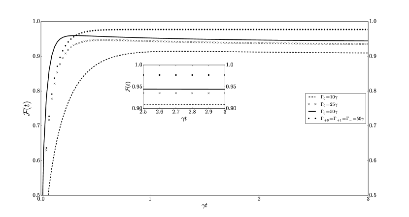
Figure 1: Evolution of the fidelity of reaching the target state $\left|\phi_{+}\right\rangle$, plotted against the scaled time $\gamma t$, from an initial thermal state with $\bar{n}=0.05$ in each cavity.

In order to investigate the possibility of reaching the state $\left|NOON\right\rangle=$ $(\left|2,0\right\rangle_{m}-\left|0,2\right\rangle_{m})/\sqrt{2}$, we have to consider two atomic beams which can, for example, each be injected through one of the cavities. We must tune one of the beams to interact with the normal mode $\overline{\omega}_{+}$ and the other with $\overline{\omega}_{-}$. Following the steps outlined above to derive master equation (7), we reach two selective Liouvillians acting in space $\left\{\left|0\right\rangle,\left|1\right\rangle\right\}$ of the modes $\overline{\omega}_{\pm}$ . In Fig.(2), we present the fidelity $\mathcal{F}(t)=\sqrt{\mathop{\mathrm{T}r}\left|NOON\right\rangle\left\langle NOON\right|\rho(t)}$ and the associated purity $\mathfrak{p}(t)=Tr\left[\rho^{2}(t)\right]$, achieved by adopting only the engineered absorption Liouvillian, with $\Gamma_{\pm 0}=50\gamma$, or both the selective absorption and emission Liouvillians, with $\Gamma_{\pm 0}=\Gamma_{\pm 1}=50\gamma$, leading to fidelities around $0.93(0.77)$ and $0.98(0.91)$, respectively. In addition to the increase in fidelity, the use of both selective Liouvillians leads to a state with a higher degree of purity.

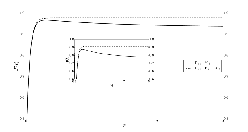
Figure 2: Evolution of the fidelity of reaching the target state $\left|NOON\right\rangle$ against the scaled time $\gamma t$, from an initial thermal state with $\bar{n}=0.05$ in each cavity. The inset shows the evolution of the purity.

Finally, we investigate the case of degenerate symmetric networks ($\omega_{m}=\omega$ and $\lambda_{mn}=\lambda)$, where the Hamiltonian (1) can be diagonalized through the canonical transformation $\ A_{1}=\frac{1}{\sqrt{N}}\sum_{m}a_{m}$ and $A_{j}=\frac{1}{\sqrt{j(j-1)}}\sum_{k=1}^{j-1}a_{k}-(j-1)a_{j}$ ($j=2,3,\ldots,N)$ and the corresponding frequencies of the normal modes are $\overline{\omega}_{1}=$ $\omega+(N+1)\lambda$ and $\overline{\omega}_{j}=$ $\omega-\lambda.\,\$Here we are interested in reaching the steady Fock state with a single excitation in the non-degenerate normal mode $\overline{\omega}_{1}$ and the vacuum state in all other degenerate modes, which corresponds to a multiqubit W-type state WCirac : $\left|1,0\ldots,0\right\rangle_{M}=\frac{1}{\sqrt{N}}(\left|1,0,\ldots,0\right\rangle_{m}+\left|0,1,\ldots,0\right\rangle_{m},\ldots,\left|0,0,\ldots,1\right\rangle_{m})=\left|W\right\rangle_{N}.$

We note that the master equation (2) for the case of degenerate symmetric networks contains only natural decay rates in the mode $\overline{\omega}_{1}$ NetoJPB , i.e. $\gamma_{1}=N\gamma$ and $\gamma_{j}=0$. Therefore, to reach the target state $\left|1,0\ldots,0\right\rangle_{M},$ in addition to the selective Lindbladian for mode $\overline{\omega}_{1}$, we need to engineer the cooling Lindbladian in mode $\overline{\omega}_{j}$. In a coupled cavity system, we can follow the same steps as those described above to construct the desired master equation:

$$\frac{d\rho}{dt} {\small=}\frac{\bar{\gamma}_{10}}{2}\left(2A_{10}^{{\dagger}}\rho A_{10}-\rho A_{10}A_{10}^{{\dagger}}-A_{10}A_{10}^{{\dagger}}\rho\right)$$

$$+(N\gamma/2)(1+\overline{n})\left(2A_{1}\rho A_{1}^{\dagger}-\rho A_{1}^{\dagger}A_{1}-A_{1}^{\dagger}A_{1}\rho\right)$$

$$+(N\gamma/2)\overline{n}\left(2A_{1}^{\dagger}\rho A_{1}-\rho A_{1}A_{1}^{\dagger}-A_{1}A_{1}^{\dagger}\rho\right),$$

$$\mathop{\displaystyle\sum}_{j}\frac{\tilde{\gamma}_{j}}{2}\left(2A_{j}\rho A_{j}^{\dagger}-\rho A_{j}^{\dagger}A_{j}-A_{j}^{\dagger}A_{j}\rho\right).$$ (8)

In Fig.(3) we present the fidelity and purity, computed from Eq.(8), of preparation of the target W-type state $\left|W\right\rangle_{N}$, for the cases $N=3,4$, adopting $\Gamma_{10},\Gamma_{j}=50\gamma$, and starting from a thermal state with $\bar{n}=0.05$. We find that the fidelities (purities) of the generated entanglements $\left|W\right\rangle_{3}$ and $\left|W\right\rangle_{4}$ are around $0.95$ $(0.81)$ and $0.94$ $(0.79)$, respectively. In the case of a degenerate linear network with a single-excitation, we can reach a set of equilibrium multiqubit states given by $\left|\Psi_{n}\right\rangle=\sqrt{(\frac{2}{N+1})}\sum_{k=1}^{N}\sin(\frac{n\pi k}{N+1})a_{k}^{\dagger}\left|0_{1},...,0_{N}\right\rangle.$

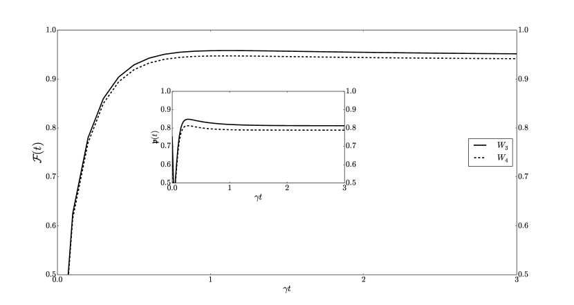
Figure 3: Evolution of the fidelity to obtain the target states $\left|W\right\rangle_{3}$ and $\left|W\right\rangle_{4}$  against the scaled time $\gamma t$, from a initial thermal state with $\bar{n}=0.05$ in each cavity. The inset gives the evolution of the purity.

We have thus advanced a theoretical proposal to obtain steady entanglements in a bosonic dissipative network in the Markovian limit. Our proposal relies on the engineering of selective JC Hamiltonians, which generate equally selective Lindblad superoperators that enable us to manipulate the equilibrium thermal distribution of the normal modes of the network. We also discuss a possible experimental implementation of our proposal in a system of coupled cavities where the required engineered Liouvillians are built from beams of three-level atoms that are made to interact with the network normal modes.

Addressing some interesting issues to be investigated further, we first observe that the role played by the network topology in the generation of the steady genuine multipartite entanglements ent was explored only slightly. Our results indicate that by manipulating the network topology, we could access a plethora of equilibrium multipartite entanglement states, covering part or all the network. Finally, it is worth investigating how the non-Markovianity and the strong interoscillator coupling regime (where the indirect dissipative channels become effective) affect our dissipative protocol for preparation of entanglements.

References

(1) For the engineering schemes relying on atomi-state
measurement, see K. Vogel, V. M. Akulin, and W. P. Schleich, Phys. Rev.
Lett. 71, 1816 (1993); R.M. Serra, N. G. de Almeida, C. J.
Villas-Boas, and M. H. Y. Moussa, Phys. Rev. A 62, 043810 (2000);
and for those not requiring atomic detection, see A. S. Parkins, P. Marte,
P. Zoller, and H. J. Kimble, Phys. Rev. Lett. 71, 3095 (1993); Th.
Wellens, A. Buchleitner, B. Kümmerer, and H. Maassen, Phys. Rev. Lett.
85, 3361 (2000).
(2) M. A. de Ponte, S. S. Mizrahi and M. H. Y. Moussa, Phys. Rev.
A 84, 012331 (2011); D. A. Lidar, I. L. Chuang, and K. B. Whaley,
Phys. Rev. Lett. 81, 2594 (1998).
(3) L. Viola and E. Knill, Phys. Rev. Lett. 94, 060502
(2005); L. C. Celeri, M. A. de Ponte, C. J. Villas-Boas, and M. H. Y.
Moussa, J. Phys. B 41, 085504 (2008).
(4) J. F. Poyatos, J. I. Cirac, and P. Zoller, Phys. Rev. Lett.
77, 4728 (1996).
(5) F. O. Prado, E. I. Duzzioni, M. H. Y. Moussa, N. G. de Almeida,
and C. J. Villas-Bôas, Phys. Rev. Lett. 102, 073008 (2009).
(6) M. Brune, E. Hagley, J. Dreyer, X. Maître, A.
Maali, C. Wunderlich, J. M. Raimond, and S. Haroche; Phys. Rev. Lett.
77, 4887–4890 (1996)
(7) M. Brune, J. Bernu, C. Guerlin, S. Dele´glise, C. Sayrin, S. Gleyzes, S. Kuhr, I. Dotsenko, J.-M. Raimond, and S.
Haroche, Phys. Rev. Lett. 101, 240402 (2008).
(8) M. Nielsen, I. Chuang, Quantum Computation and
Quantum Information, Cambridge University Press, 2000, 409-416.
(9) C. J. Myatt, B. E. King, Q. A. Turchette, C. A. Sackett. D.
Kielpinski, W. M. Itano, C. Monroe, and D. J. Wineland, Nature 403,
269 (2000).
(10) S. Diehl, A. Micheli, A. Kantian, B. Kraus, H. P. Buchler, and
P. Zoller, Nature phys. 4, 878 (2008); B. Kraus, H. P. Büchler,
S. Diehl, A. Kantian, A. Micheli, and P. Zoller1, Phys. Rev. A 78,
042307 (2008); M. Müller, S. Diehl, G. Pupillo, P. Zoller, Adv. At. Mol.
Opt. Phys. 61, 1 (2012).
(11) M. J. Kastoryano, F. Reiter, and A. S. Sørensen,Phys. Rev.
Lett. 106, 090502 (2011); A. F. Alharbi and Z. Ficek, Phys. Rev. A
82, 054103 (2010).
(12) X. Chen, L. Shen, Z. Yang, H. Wu and M. Chen, J. Opt. Soc.
Am. B 29, 1535 (2012); R. Sweke, I. Sinayskiy, and F. Petruccione,
Phys. Rev. A 87, 042323 (2013).
(13) J. Cho, S. Bose, and M. S. Kim. Phys. Rev. Lett., 106, 020504 (2011); K. Stannigel, P. Rabl, and P. Zoller, New J. Phys. 14, 063014 (2012).
(14) K. L. Liu, H. S. Goan, Phys. Rev. A 76, 022312
(2007); G. X. Li, L. H. Sun, Z. Ficek, J. Phys. B 43, 135501 (2010).
(15) M. Delanty and K. Ostrikov, Eur. Phys. J. D 67,
193 (2013).
(16) F. O. Prado, W. Rosado, G. D. de Moraes Neto and M. H. Y.
Moussa, Europh. Lett. 107, 13001(2014).
(17) F. O. Prado, W. Rosado, A. M. Alcalde, and M. H. Y.
Moussa, J. Phys. B: At. Mol. Opt. Phys. 46, 205501 (2013).
(18) J. M. Raimond, M. Brune, and S. Haroche, Rev. Mod. Phys.
73, 565 (2001).
(19) S. Pielawa, G. Morigi, D. Vitali, and L. Davidovich, Phys. Rev.
Lett. 98, 240401 (2007); S. Pielawa, L. Davidovich, D. Vitali, and G.
Morigi, Phys. Rev. A 81, 043802 (2010); S. Pielawa, G. Morigi, D.
Vitali, and L. Davidovich, Phys. Rev. A 85, 022120 (2012);B.-G.
Englert and G. Morigi, in Coherent Evolution in Noisy Environments, edited
by A. Buchleitner and K. Hornberger (Springer, Berlin, 2002), p. 55.
(20) R. F. Rossetti et al., arXiv:1409.2691 (to appear in Phys.
Rev. A).
(21) J. Q. You, Y. X. Liu, and F. Nori, Phys. Rev. Lett. 100, 047001 (2008).
(22) M. A. de Ponte , S. S. Mizrahi and M. H. Y. Moussa, J. Phys.
A: Math. Theor. 42, 365304 (2009).
(23) B. F. C. Yabu-uti, and J. A. Roversi, Quantum Inf Process
12, 189 (2013); A. Serafini , S. Mancini and S. Bose, Phys. Rev.
Lett. 96 010503 (2006).
(24) O. Gamel and D. F. V. James, Phys. Rev. A 82,
052106 (2010); D. F. V. James and J. Jerke, Can. J. Phys. 85, 625
(2007).
(25) J. R. Johansson, P. D. Nation, and F. Nori, Comput. Phys.
Commun. 183, 1760 (2012); ibid. 184, 1234 (2013).
(26) G. D. M. Neto et al., J. Phys. B 44, 145502
(2011).
(27) W. Dür, G. Vidal and J. I. Cirac, Phys. Rev. A 62, 062314 (2000).
(28) P. Van Loock, A. Furusawa, Phys. Rev. A 67, 52315 (2003); U.
Marzolino, Europh. Lett. 104, 40004 (2013).