Elementary solution to the time-independent quantum navigation problem

Abstract

A quantum navigation problem concerns the identification of a time-optimal Hamiltonian that realises a required quantum process or task, under the influence of a prevailing ‘background’ Hamiltonian that cannot be manipulated. When the task is to transform one quantum state into another, finding the solution in closed form to the problem is nontrivial even in the case of time-independent Hamiltonians. An elementary solution, based on trigonometric analysis, is found here when the Hilbert space dimension is two. Difficulties arising from generalisations to higher-dimensional systems are discussed.

Motivated in part by the advances in quantum technologies, significant progress has been made in finding the time-optimal scheme to implement a unitary operation that achieves the transformation of one quantum state into another, subject to a given set of constraints ML ; lloyd1 ; brockett ; brody1 ; lloyd3 ; hosoya ; brody2 ; hosoya2 ; zanardi ; caneva ; GCH ; garon ; stepney1 ; lloyd . Typically it is assumed that external influences such as a background field or potential are absent, but in some cases it can be difficult to eliminate ‘ambient’ Hamiltonians in a laboratory. In such a context, Russell & Stepney stepney2 considered a time-minimisation problem of transporting one unitary operator ${\hat{U}}_{I}$ into another operator ${\hat{U}}_{F}$, subject to the existence of a background Hamiltonian ${\hat{H}}_{0}$ that cannot be manipulated. The task here therefore is to find the (time-dependent) control Hamiltonian ${\hat{H}}_{1}(t)$ such that ${\hat{H}}={\hat{H}}_{0}+{\hat{H}}_{1}$ transforms ${\hat{U}}_{I}$ into ${\hat{U}}_{F}$ in the shortest possible time. Evidently, there has to be a bound on the energy resource, which in their problem is given by the trace norm of the control—the ‘full throttle’ condition: ${\rm tr}({\hat{H}}_{1}^{2})=1$ at all time. In addition, to ensure the existence of viable controls it is assumed that the background Hamiltonian is not dominant, i.e. ${\rm tr}({\hat{H}}_{0}^{2})<1$. Inspired by the classical problem of navigation in the ocean in the presence of wind or currents zermelo ; caratheodory , this is referred to as the quantum Zermelo navigation problem stepney2 . The solution to this problem of constructing a unitary gate under an external field was obtained recently stepney3 ; brody3 , whereas the problem of finding the time-optimal transformation $|\psi_{I}\rangle\to|\psi_{F}\rangle$ of quantum states under a similar setup has not yet been solved.

\begin{overpic}[scale={0.40}]{figure0.pdf}\put(44.2,63.5){$\psi_{I}$} \put(49.2,61.5){$\bullet$}\put(44.2,27.6){$\psi_{F}$} \put(49.2,29.2){$\bullet$}\end{overpic}

Figure 1: Circles on the sphere passing through a pair of points. It is evident that the totality of latitudinal circles passing through the two points $|\psi_{I}\rangle$ and $|\psi_{F}\rangle$ share the property that the axes perpendicular to the circles lie on the plane that bisects all the circles.

In the present paper we investigate an analogous problem of finding the time-optimal control Hamiltonian ${\hat{H}}_{1}$ that achieves the transformation $|\psi_{I}\rangle\to|\psi_{F}\rangle$, subject to the existence of an ambient Hamiltonian ${\hat{H}}_{0}$, but in the time-independent context. It turns out that when ${\hat{H}}_{1}$ cannot vary in time, then the problem of finding the ‘time-optimal’ control that generates a given unitary gate ${\hat{U}}_{I}\to{\hat{U}}_{F}$ becomes trivial (shown below), while that of finding the optimal control to generate the transformation $|\psi_{I}\rangle\to|\psi_{F}\rangle$ remains nontrivial. Nevertheless, in the case of two-level systems, on account of the fact that the configuration of the states can be ‘visualised’ on a Bloch sphere, we are able to derive an elementary solution that requires nothing more than trigonometric manipulations. Our solution in fact extends to higher dimensions if the background Hamiltonian ${\hat{H}}_{0}$ (‘wind’) happens to leave invariant the Hilbert subspace spanned by the given two states $|\psi_{I}\rangle$ and $|\psi_{F}\rangle$; whereas the solution to the more general cases in higher dimensions remains open.

We begin our analysis by remarking that if a time-independent Hamiltonian ${\hat{H}}={\hat{H}}_{0}+{\hat{H}}_{1}$ were to transform $|\psi_{I}\rangle$ into $|\psi_{F}\rangle$ in a two-dimensional Hilbert space, then since the action of ${\hat{H}}$ amounts to a rigid rotation of the associated Bloch sphere about some axis, the two states $|\psi_{I}\rangle$ and $|\psi_{F}\rangle$ must lie on the same latitudinal circle with respect to the axis of rotation determined by ${\hat{H}}$. A set of such circles is sketched in figure 1. Therefore, the totality of rotation axes permitting such transformations lie on the great circle passing the point $\frac{1}{\sqrt{2}}(|\psi_{I}\rangle+|\psi_{F}\rangle)$ that is orthogonal to the great circle joining the two points on the Bloch sphere corresponding to the states $|\psi_{I}\rangle$ and $|\psi_{F}\rangle$. Without loss of generality, let us work in the frame such that the two states can be expressed in the form

$$|\psi_{I}\rangle=\left(\!\begin{array}[]{c}\cos\frac{1}{4}(\pi-\theta)\\ \\ \sin\frac{1}{4}(\pi-\theta)\end{array}\!\right),\quad|\psi_{F}\rangle=\left(\!\begin{array}[]{c}\cos\frac{1}{4}(\pi+\theta)\\ \\ \sin\frac{1}{4}(\pi+\theta)\end{array}\!\right),$$ (7)

where $\theta$ is the angular separation of the two states $|\psi_{I}\rangle$ and $|\psi_{F}\rangle$. In other words, we work with the coordinates such that both the initial and the target states lie on a longitudinal great circle, and such that the equator bisects the join of $|\psi_{I}\rangle$ and $|\psi_{F}\rangle$. By embedding the Bloch sphere in ${\mathds{R}}^{3}$ we then find that the two points on the sphere corresponding to the vectors $|\psi_{I}\rangle$ and $|\psi_{F}\rangle$ lie on the $xz$-plane, located symmetrically about the $xy$-plane. Writing $\boldsymbol{\psi}_{I}$ and $\boldsymbol{\psi}_{F}$ for the two vectors in ${\mathds{R}}^{3}$ corresponding to the two states, we thus have

$$\boldsymbol{\psi}_{I}=\frac{1}{2}\left(\begin{array}[]{c}\cos\frac{\theta}{2}\\ 0\\ \sin\frac{\theta}{2}\end{array}\right),\qquad\boldsymbol{\psi}_{F}=\frac{1}{2}\left(\begin{array}[]{c}\cos\frac{\theta}{2}\\ 0\\ -\sin\frac{\theta}{2}\end{array}\right),$$ (14)

since the radius of the Bloch sphere is $\frac{1}{2}$. This configuration is schematically illustrated in figure 2.

With the above choice of coordinates it should be evident that any rotation of the sphere about an axis that lies on the $xy$-plane will in time transport $|\psi_{I}\rangle$ into $|\psi_{F}\rangle$. Conversely, no rotation about an axis that does not lie on the $xy$-plane will ever transport $|\psi_{I}\rangle$ into $|\psi_{F}\rangle$. In the absence of the background ‘wind’ ${\hat{H}}_{0}$, therefore, if the objective is to minimise the time subject to finite energy resource, then since the voyage time is the distance divided by speed, a priori one has to deal with a complicated optimisation problem of minimising this ratio. However, fortunately in the case of a unitary evolution, the path that minimises the distance is precisely the path that maximises the evolution speed brody1 , so there is no need to evoke a simultaneous optimisation; all one needs is to find the shortest path. But geodesic curves on a sphere are given by the great circles, so without any calculation it is clear that the optimal Hamiltonian is given by the one corresponding to a rotation about the $y$-axis brody2 .

Figure 2: Configuration of the initial and target states. Since the action of a time-independent Hamiltonian ${\hat{H}}={\boldsymbol{r}}\cdot{\hat{\boldsymbol{\sigma}}}$ amounts to a rigid rotation of the Bloch sphere, if the unitary operator $\mbox{$\rm e$}^{-{\rm i}{\hat{H}}t}$ were to transform a given initial state $|\psi_{I}\rangle$ into a target final state $|\psi_{F}\rangle$ at some time, the axis ${\boldsymbol{r}}$ of rotation has to lie on the equator that bisects the great circle joining $|\psi_{I}\rangle$ and $|\psi_{F}\rangle$. When ${\boldsymbol{r}}$ points in the direction of the $y$-axis, the orbit $|\psi(t)\rangle=\mbox{$\rm e$}^{-{\rm i}{\hat{H}}t}|\psi_{I}\rangle$ is a geodesic curve, but owing to the prevailing ‘wind’ ${\hat{H}}_{0}$, the journey along the shortest path does not result in the shortest time.

In the presence of a background wind ${\hat{H}}_{0}$, however, the situation is different: In this case, depending on the choice of ${\hat{H}}$, that is, the choice of the rotation axis on the $xy$-plane, the energy resource available to the Hamiltonian ${\hat{H}}$ is different. As a consequence, one can find a Hamiltonian ${\hat{H}}$ such that although the path $|\psi(t)\rangle$ joining $|\psi_{I}\rangle$ and $|\psi_{F}\rangle$ is not the shortest, there is sufficient energy resource to overcome the extra mileage such that the voyage time will be shorter than that corresponding to the rotation about the $y$-axis. The objective, therefore, is to find the axis for which the voyage time is minimised.

With these observations at hand, let us write the background Hamiltonian ${\hat{H}}_{0}$ in the form

$${\hat{H}}_{0}=\sqrt{\frac{\epsilon}{2}}\big{(}x{\hat{\sigma}}_{x}+y{\hat{\sigma}}_{y}+z{\hat{\sigma}}_{z}\big{)},$$ (15)

where $x^{2}+y^{2}+z^{2}=1$ and where $0<\epsilon<1$. It follows that ${\rm tr}({\hat{H}}_{0}^{2})=\epsilon<1$. Whatever the control Hamiltonian ${\hat{H}}_{1}$ might be, the total Hamiltonian has to take the form

$${\hat{H}}=\frac{\omega}{2}\big{(}\cos\phi\,{\hat{\sigma}}_{x}+\sin\phi\,{\hat{\sigma}}_{y}\big{)}$$ (16)

for some $\omega$ satisfying the constraint. In other words, the axis of rotation generated by ${\hat{H}}$ is at some angle $\phi$ from the $x$-axis on the $xy$-plane. Since ${\hat{H}}_{1}={\hat{H}}-{\hat{H}}_{0}$, the constraint ${\rm tr}({\hat{H}}_{1}^{2})=1$ on the control Hamiltonian implies that

$$\omega^{2}-2\sqrt{2\epsilon}(x\cos\phi+y\sin\phi)\omega-2(1-\epsilon)=0.$$ (17)

We shall find that the voyage time $\tau$ such that the condition $\mbox{$\rm e$}^{-{\rm i}{\hat{H}}\tau}|{\psi}_{I}\rangle=|{\psi}_{F}\rangle$ is met will also depend on the variables $\omega$ and $\phi$. Thus, our objective is to minimise $\tau$ subject to the constraint (17).

It should be remarked parenthetically that we have chosen both ${\hat{H}}_{0}$ and ${\hat{H}}_{1}$ be trace free. This is because a physically meaningful constraint on the energy resource, in the case of a quantum system modelled on a finite-dimensional Hilbert space, is linked to the gap between the highest and the lowest attainable energy eigenvalues, not to the value of the ground-state energy brody1 . We shall therefore be working, without loss of generality, with trace-free Hamiltonians.

To proceed, it should be evident from the foregoing formulation that the voyage time is proportional to the angle, call it $\alpha$, of rotation about the ${\hat{H}}$-axis that turns the vector $\boldsymbol{\psi}_{I}$ into $\boldsymbol{\psi}_{F}$ in ${\mathds{R}}^{3}$. Specifically, since the angular frequency generated by the Hamiltonian ${\hat{H}}$ of (16) is $\omega$, this in turn determines the voyage time according to the relation $\alpha=\omega t$. It follows that the problem reduces to working out elementary trigonometric relations. Let us define the vector ${\boldsymbol{r}}$ by

$${\boldsymbol{r}}=\frac{\omega}{2}\left(\begin{array}[]{c}\cos\phi\\ \sin\phi\\ 0\end{array}\right)$$ (21)

so that ${\hat{H}}={\boldsymbol{r}}\cdot{\hat{\boldsymbol{\sigma}}}$. Thus ${\boldsymbol{r}}$ determines the axis of rotation in ${\mathds{R}}^{3}$ generated by ${\hat{H}}$. To determine $\alpha$, let us first identify the angular separation $\rho$ between ${\boldsymbol{r}}$ and $\boldsymbol{\psi}_{I}$ (which, of course, is the same as that between ${\boldsymbol{r}}$ and $\boldsymbol{\psi}_{F}$ on account of the symmetry). To assist the analysis, in figure 3 we give the perspective of the configuration around the ${\boldsymbol{r}}$-axis. Since ${\boldsymbol{r}}\cdot\boldsymbol{\psi}_{I}=|{\boldsymbol{r}}|\,|\boldsymbol{\psi}_{I}|\,\cos\rho$, we find

$$\cos\rho=\cos\phi\cos\mbox{$\textstyle\frac{1}{2}$}\theta.$$ (22)

The final step required is to identify the vector ${\boldsymbol{c}}$ depicted in figure 3 that points in the direction of ${\boldsymbol{r}}$ such that the two points $\boldsymbol{\psi}_{I}$ and $\boldsymbol{\psi}_{F}$ lie on the plane perpendicular to ${\boldsymbol{r}}$ at ${\boldsymbol{c}}$. But clearly this is given by

$${\boldsymbol{c}}=\mbox{$\textstyle\frac{1}{2}$}\cos\rho\left(\begin{array}[]{c}\cos\phi\\ \sin\phi\\ 0\end{array}\right),$$ (26)

from which it follows, after some algebra, that

$$\cos\alpha = \frac{\boldsymbol{\psi}_{I}-{\boldsymbol{c}}}{|\boldsymbol{\psi}_{I}-{\boldsymbol{c}}|}\cdot\frac{\boldsymbol{\psi}_{F}-{\boldsymbol{c}}}{|\boldsymbol{\psi}_{F}-{\boldsymbol{c}}|}$$ (27)

$$= \frac{\sin^{2}\phi-\tan^{2}\frac{\theta}{2}}{\sin^{2}\phi+\tan^{2}\frac{\theta}{2}}.$$

As indicated above, since the angular frequency is $\omega$, the first time $\tau$ at which the state $|\psi_{I}\rangle$ is turned into $|\psi_{F}\rangle$ is given by $\omega\tau=\alpha$, that is,

$$\tau=\frac{1}{\omega}\,\cos^{-1}\left(\frac{\sin^{2}\phi-\tan^{2}\frac{\theta}{2}}{\sin^{2}\phi+\tan^{2}\frac{\theta}{2}}\right).$$ (28)

On the other hand, the constraint (17) allows us to express $\omega$ in terms of $\phi$. Putting these together, the first voyage time $\tau=\tau(\phi)$ can be expressed explicitly as a function of the angle $\phi$ that determines the axis of rotation generated by ${\hat{H}}$, which in turn determines ${\hat{H}}_{1}$. Specifically, we have

$$\omega = \sqrt{2\epsilon(x\cos\phi+y\sin\phi)^{2}+2(1-\epsilon)}$$ (29)

$$\quad+\sqrt{2\epsilon}(x\cos\phi+y\sin\phi),$$

which together with (28) gives $\tau(\phi)$, and this in turn must be minimised for fixed $x$, $y$, $\epsilon$ and $\theta$.

Figure 3: Identification of the rotation angle. The angle $\alpha$ of rotation about the ${\boldsymbol{r}}$-axis required to turn the vector ${\boldsymbol{\psi}}_{I}$ into ${\boldsymbol{\psi}}_{F}$ is determined by first identifying the vector ${\boldsymbol{c}}$ such that ${\boldsymbol{\psi}}_{I}-{\boldsymbol{c}}\perp{\boldsymbol{r}}$. Then we have $({\boldsymbol{\psi}}_{I}-{\boldsymbol{c}})\cdot({\boldsymbol{\psi}}_{F}-{\boldsymbol{c}})\propto\cos\alpha$, from which $\alpha$ can be obtained.

In figure 4 we plot $\tau(\phi)$ as a function of $\phi$ for a choice of parameters $x$, $y$, $\epsilon$ and $\theta$. Since the problem is reduced to a one-dimensional minimisation task, the optimal value $\phi^{*}$ for the axis of rotation can easily be determined numerically, which, when substituted in (29) and in (16), identifies the optimal overall Hamiltonian ${\hat{H}}(\phi^{*})$, from which the optimal control can be determined by the relation ${\hat{H}}_{1}(\phi^{*})={\hat{H}}(\phi^{*})-{\hat{H}}_{0}$. This completes our analysis of finding the time-optimal Hamiltonian that generates the transformation $|\psi_{I}\rangle\to|\psi_{F}\rangle$ of quantum states, subject to the existence of a prevailing ‘wind’ ${\hat{H}}_{0}$. As for the time required to achieve the transformation, this is given by $\tau(\phi^{*})$.

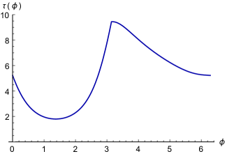
Figure 4: Voyage time $\tau(\phi)$ as a function of the angle $\phi$. As the axis of rotation generated by ${\hat{H}}$, parameterised by $\phi$, is varied, the voyage time changes accordingly. Here, as an example, we plot $\tau(\phi)$ for the parameter choice: $x=0.1$, $y=0.23$, $z=(1-x^{2}-y^{2})^{\frac{1}{2}}\approx 0.97$, $\epsilon=0.9$, and $\theta=\pi/2$. In this example, the optimal angle is $\phi^{*}\approx 0.44\,\pi$. At $\phi=\pi$ there is a cusp (irrespective of the parameter values), since the orientation of the path $|\psi(t)\rangle=\mbox{$\rm e$}^{-{\rm i}{\hat{H}}t}|\psi_{I}\rangle$ changes as $\phi$ passes through $\pi$.

We conclude by remarking on the generalisation to higher dimensions, as well as on the problem of optimally generating a given unitary gate. In either case, in the time-independent context the evolution operator is given by $\mbox{$\rm e$}^{-{\rm i}{\hat{H}}T}$ for some Hamiltonian ${\hat{H}}$ and voyage time $T$. Thus the task is to find the best choice of ${\hat{H}}$ that minimises $T$ such that either

$$\mbox{$\rm e$}^{-{\rm i}{\hat{H}}T}|{\psi}_{I}\rangle=|{\psi}_{F}\rangle$$ (30)

or

$$\mbox{$\rm e$}^{-{\rm i}{\hat{H}}T}{\hat{U}}_{I}={\hat{U}}_{F},$$ (31)

is realised, depending on which problem one is considering. Now for a system modelled on an $n$-dimensional Hilbert space, the space of pure states is the associated projective Hilbert space of $n-1$ complex dimensions. Thus, the specification of a state requires the specification of $2n-2$ degrees of freedom. On the other hand, the specification of a Hamiltonian, up to trace, requires $n^{2}-1$ degrees of freedom. Together with the fact that $T$ is also unknown, we have, in (30), $n^{2}$ unknowns; while, noting that there is also the trace-norm condition, there are $(2n-2)+1=2n-1$ conditions. It follows that the solution to the problem of the type (30) involves an optimisation over $n^{2}-(2n-1)=(n-1)^{2}$ parameters, which in general is nontrivial. For $n=2$, this reduces to a single-parameter optimisation, and an explicit representation of $\tau$ in terms of trigonometric functions can be found, as shown above. For $n>2$, our solution remains valid if ${\hat{H}}_{0}$ leaves invariant the two-dimensional Hilbert subspace spanned by $|{\psi}_{I}\rangle$ and $|{\psi}_{F}\rangle$, on account of the observation made in brody2 ; whereas in the general case, the voyage time $\tau$ will depend on $(n-1)^{2}$ parameters, hence a numerical search in a higher-dimensional parameter space is required to identify the optimal $\tau^{*}$. It remains open whether a similarly simple analytical form of $\tau$ can be found in higher dimensions. In any event, the problem of the kind represented in (30) is in general nontrivial, even in the time-independent context. As for the construction of a unitary gate as in (31), on the other hand, the situation is markedly different. Here the number of unknowns remains the same, but the number of constraints in (31), together with the trace condition, completely counterbalances this (recall that while (30) is a vector relation, (31) is a matrix relation), and there is no degree of freedom left to optimise. That is, the optimal Hamiltonian is given exactly by ${\hat{H}}^{*}=\mbox{$\rm i$}T^{-1}\ln({\hat{U}}_{F}{\hat{U}}_{I}^{-1})$, where $T$ is fixed by the trace-norm condition. Specifically, writing ${\hat{X}}=\mbox{$\rm i$}\ln({\hat{U}}_{F}{\hat{U}}_{I}^{-1})$ for simplicity, we have, on account of ${\rm tr}({\hat{H}}_{1}^{2})={\rm tr}((T^{-1}{\hat{X}}-{\hat{H}}_{0})^{2})=1$,

$$\frac{1}{T}=\frac{\sqrt{({\rm tr}({\hat{H}}_{0}{\hat{X}}))^{2}+[1-{\rm tr}({\hat{H}}_{0}^{2})]{\rm tr}({\hat{X}}^{2})}+{\rm tr}({\hat{H}}_{0}{\hat{X}})}{{\rm tr}({\hat{X}}^{2})}\,\,\,$$ (32)

for the voyage time required to realise the transformation ${\hat{U}}_{I}\to{\hat{U}}_{F}$. Thus, in the case of time-independent Hamiltonians, the problem of finding a time-optimal Hamiltonian to generate a unitary gate, under the influence of a background Hamiltonian ${\hat{H}}_{0}$, is empty—only with a time-dependent control ${\hat{H}}_{1}(t)$ the ‘bound’ in (32) can be overcome stepney3 ; brody3 .

References

- (1) Margolus, N. & Levitin, L. B. 1998 The maximum speed of dynamical evolution. Physica D120, 188.
- (2) Lloyd, S. 1999 Ultimate physical limits to computation. Nature 406, 1047.
- (3) Khaneja, N., Glaser, S. J. & Brockett, R. 2002 Sub-Riemannian geometry and time optimal control of three spin systems: Quantum gates and coherence transfer. Phys. Rev. A65, 032301.
- (4) Brody, D. C. 2003 Elementary derivation for passage time. J. Phys. A36, 5587.
- (5) Giovannetti, V., Lloyd, S. & Maccone, L. 2003 Quantum limits to dynamical evolution. Phys. Rev. A67, 052109.
- (6) Carlini, A., Hosoya, A., Koike, T. & Okudaira, Y. 2006 Time-optimal quantum evolution. Phys. Rev. Lett. 96, 060503.
- (7) Brody, D. C. & Hook, D. W. 2006 On optimum Hamiltonians for state transformations. J. Phys. A39, L167.
- (8) Carlini, A., Hosoya, A., Koike, T. & Okudaira, Y. 2007 Time-optimal unitary operations. Phys. Rev. A75, 042308.
- (9) Rezakhani, A. T., Kuo, W. J., Hamma, A., Lidar, D. A. & Zanardi, P. 2009 Quantum adiabatic brachistochrone. Phys. Rev. Lett. 103, 080502.
- (10) Caneva, T., Murphy, M., Calarco, T., Fazio, R., Montangero, S., Giovannetti, V. & Santoro, G. E. 2009 Optimal control at the quantum speed limit. Phys. Rev. Lett. 103, 240501.
- (11) Hegerfeldt, G. C. 2013 Driving at the quantum speed limit: Optimal control of a two-level system. Phys. Rev. Lett. 111, 260501.
- (12) Garon, A., Glaser, S. J. & Sugny, D. 2013 Time-optimal control of SU(2) quantum operations. Phys. Rev. A88, 043422.
- (13) Russell, B. & Stepney, S. 2013 Geometric methods for analysing quantum speed limits: Time-dependent controlled quantum systems with constrained control functions. In Unconventional Computation and Natural Computation, G. Mauri, et al. Eds., (Berlin: Springer-Verlag).
- (14) Wang, X., Allegra, A., Jacobs, K., Lloyd, S., Lupo, C. & Mohseni, M. 2014 Quantum brachistochrone curves as geodesics: obtaining accurate control protocols for time-optimal quantum gates. arXiv:1408.2465
- (15) Russell, B. & Stepney, S. 2014 Zermelo navigation and a speed limit to quantum information processing. Phys. Rev. A90, 012303.
- (16) Zermelo, E. 1931 Über das Navigationsproblem bei ruhender oder veränderlicher Windverteilung. Ztschr. f. angew. Math. und Mech. 11, 114.
- (17) Carathéodory, C. 1935 Variationsrechnung und Partielle Differentialgleichungen erster Ordnung. (Berlin: B. G. Teubner).
- (18) Russell, B. & Stepney, S. 2014 Zermelo navigation in the quantum brachistochrone. arXiv:1409.2055
- (19) Brody, D. C. & Meier, D. M. 2014 Solution to the quantum Zermelo navigation problem. arXiv:1409.3204