Quantum correlation evolution of GHZ and W states under noisy channels using ameliorated measurement-induced disturbance

Abstract

We study quantum correlation of Greenberger-Horne-Zeilinger (GHZ) and W states under various noisy channels using measurement-induced disturbance approach and its optimized version. Although these inequivalent maximal entangled states represent the same quantum correlation in the absence of noise, it is shown that the W state is more robust than the GHZ state through most noisy channels. Also, using measurement-induced disturbance measure, we obtain the analytical relations for the time evolution of quantum correlations in terms of the noisy parameter $\kappa$ and remove its overestimating quantum correlations upon implementing the ameliorated measurement-induced disturbance.

I Introduction

Quantification of correlations in bipartite quantum systems is one of the important problems in quantum information. Quantum correlations can be considered as the resources for quantum information processes nel . Initially, it was assumed that entanglement which plays an important role in quantum computing and quantum information processing, is the only kind of nonclassical correlation in a quantum state. This issue has been widely studied in the last decade and various entanglement measures have been introduced to measure entanglement such as entanglement of formation, entanglement of cost, relative entropy entanglement, and negativity.

Indeed, entanglement is not the only responsible correlation for the quantum bypassing classical regimes and there exists some quantum correlations other than entanglement which result in the quantum effects in quantum information processes. For instance, Bennett et al. showed the possibility of quantum nonlocality without entanglement bennett99 . Also, it is shown that separable states can be used for quantum speedup braun99 ; meyer00 ; biham04 ; datta0507 . In order to quantify the quantumness of correlations in bipartite states, it has been proposed several measures such as quantum discord ollivier01 , quantum deficit raja02 ; horodecki05 ; devetak05 , quantumness of correlations usha08 , and quantum dissonance modi10 .

In particular, quantum discord which historically is the first introduced measure for the nonclassicality based on the Openheim-Horodecki paradigm, has attracted much attention in recent years shabani09 ; rulli11 ; giorda12 ; terzis12 ; joao13 . It is based on the difference between two quantum extensions of classically equivalent concepts namely the mutual information. Although quantum discord has a simple definition, its explicit evaluation is hard to perform in practice especially for multi-qubit states and is often only given by numerical methods. However, some analytical expression of quantum discord for two-qubit states are presented in Refs. d1 ; d2 ; d3 ; d4 ; d5 .

It is known that since some separable states still have quantum correlations, these correlations with quantum nature are more general than entanglement. In particular, Luo luo08 introduced a quantum-classical classification based on measurement-induced disturbance (MID) to characterize statistical correlations in bipartite states. In this scenario, classical states are classified in terms of nondisturbance under quantum measurement. However, quantum systems and thus quantum correlations are disturbed under generic measurements and the magnitude of the disturbance can be considered as a measure to characterize the quantumness of states. Recently, Girolami et al. showed that the quantum discord due to its asymmetric definition does not properly determine the distinction between classical-classical and classical-quantum states and thus it is not strongly faithful. Also, by characterizing quantum correlations in the paradigmatic instance of two-qubit states, they observed that MID overstimates quantum correlations so that for some classical states we obtain nonzero correlation. They therefore proposed an ameliorated measurement-induced disturbance (AMID) as a quantifier of quantum correlations girolami11 .

The aim of this paper is to characterize and quantify the quantum correlation for bipartite systems which are initially prepared in three-qubit Greenberger-Horne-Zeilinger (GHZ) ghz89

$$|\mbox{GHZ}\rangle=\frac{|000\rangle+|111\rangle}{\sqrt{2}},$$ (1)

and W dur00 ; pati

$$|W\rangle=\frac{|100\rangle+|010\rangle+{\sqrt{2}}|001\rangle}{2},$$ (2)

states under various noisy channels where the first two qubits belong to party $a$ and the third qubit belongs to party $b$. It is shown that this class of W states can be used for perfect teleportation, superdense coding, and as an entanglement resource pati . This state belongs to the category of W states

$$|W_{n}\rangle=\frac{|100\rangle+\sqrt{n}e^{i\gamma}|010\rangle+{\sqrt{n+1}}e^{i\delta}|001\rangle}{\sqrt{2+2n}},$$ (3)

where $n$ is a real number, $\delta$ and $\gamma$ are phases, and reduces to $|W\rangle$ for $n=1$ and zero phases. Then, the initial states are affected by noisy channels which results in decreasing of the quantumness of states. We quantify the quantum correlations for the initial GHZ and W states in the presence of noise and investigate the robustness of these states under different kinds of noise. The rest of this paper is organized as follows. In Sec. II, we characterize quantum correlations using MID and AMID approaches. Secs. III and IV are devoted to determine quantum correlations for the GHZ and W states, respectively. We present our conclusions in Sec. V.

II Classifying bipartite states using ameliorated measurement-induced disturbance

Consider a bipartite state $\rho$ for a system with two parties $a$ and $b$. Based on measurement-induced disturbance, the quantum correlations of $\rho$, that is denoted by ${\cal M}(\rho^{ab})$, is given by luo08

$${\cal M}(\rho^{ab})=I(\rho^{ab})-I(\Pi(\rho^{ab})),$$ (4)

where $I(\rho^{ab})=S(\rho^{a})+S(\rho^{b})-S(\rho^{ab})$ is quantum mutual information that quantifies the total correlation between $a$ and $b$, and

$$\Pi(\rho)=\sum_{ij}(\Pi_{a,i}\otimes\Pi_{b,j})\,\rho\,(\Pi_{a,i}\otimes\Pi_{b,j}),$$ (5)

in which $\{\Pi_{a,i}\}$ and $\{\Pi_{b,j}\}$ are complete projective measurements for parties $a$ and $b$, respectively. They are obtained from the spectral decomposition of the reduced states, namely $\rho^{a}=\sum_{i}p_{a,i}\Pi_{a,i}$ and $\rho^{b}=\sum_{j}p_{b,j}\Pi_{b,j}$. We can rewrite Eq. (4) as

$${\cal M}(\rho^{ab})=S(\Pi(\rho^{ab}))-S(\rho^{ab})+\sum_{i}(S(\rho^{x_{i}})-S(\Pi(\rho^{x_{i}}))$$ (6)

where $x_{i}\in\{a,b\}$. Note that if $\Pi(\rho)=\rho$, we conclude $\rho$ is not perturbed with respect to local measurement $\Pi_{a,i}\otimes\Pi_{b,j}$, therefore $\rho$ is a classical state. Otherwise, it is a quantum state and possesses quantum correlation. For our case, since party $a$ has two qubits, it is convenient to write Eq. (5) as $\Pi(\rho)=\sum_{ijk}(\Pi_{a,{ij}}\otimes\Pi_{b,k})\,\rho\,(\Pi_{a,{ij}}\otimes\Pi_{b,k})$. Also, we define $\Pi_{\bf n}=\Pi_{a,{ij}}\otimes\Pi_{b,k}$ so that the projective measurements satisfy $\Pi_{\bf n}\Pi_{{\bf n^{\prime}}}=\delta_{{\bf nn^{\prime}}}\Pi_{\bf n}$ and $\sum_{\bf n}\Pi_{\bf n}=1$.

According to AMID, Eq. (6) needs to optimize over any possible set of local projectors so that projective measurement in this equation, which we represent by $\Omega$ instead of $\Pi$, includes arbitrary complete projective measurements that are not necessarily obtained from eigen-projectors. Therefore, the quantum correlation which is denoted by ${\cal A}(\rho^{ab})$, is given by girolami11

$${\cal A}(\rho^{ab})=\inf_{\Omega}\left[S(\Omega(\rho^{ab}))-S(\rho^{ab})+\sum_{i}(S(\rho^{x_{i}})-S(\Omega(\rho^{x_{i}}))\right],$$ (7)

in which

$$\Omega(\rho)=\sum_{ij}(\Omega_{a,i}\otimes\Omega_{b,j})\,\rho\,(\Omega_{a,i}\otimes\Omega_{b,j}),$$ (8)

$\Omega_{j,k}=U_{j}\Pi_{j,k}U_{j}^{\dagger}$, and $U_{j}=y_{j,0}I+i\vec{\bf{y}}_{j}.\vec{\bf{\sigma}}_{j}$ is a unitary matrix obeys $\sum_{p=0}^{3}y_{j,p}^{2}=1$, $y_{j,p}\in[-1,1]$.

The evolution of the quantum system $\rho$ in the presence of noise is given by the master equation in the Lindblad form lind76

$$\frac{\partial\rho}{\partial t}=-\frac{i}{\hbar}[H_{S},\rho]+\sum_{i,\alpha}\left(L_{i,\alpha}\rho L_{i,\alpha}^{\dagger}-\frac{1}{2}\left\{L_{i,\alpha}^{\dagger}L_{i,\alpha},\rho\right\}\right),$$ (9)

in which the effect of noise is presented by the Lindblad operator $L_{i,\alpha}$ that acts on the $i$th qubit, $\alpha$ determines the type of the noise, and $H_{S}$ is the Hamiltonian of the system. In Ref. jung08 , the authors studied analytic solutions of the Lindblad equation for GHZ and W states under various noises for $H_{S}=0$ and same axis Pauli noises by taking $L_{i,\alpha}=\sqrt{\kappa_{i,\alpha}}\sigma^{(i)}_{\alpha}$ where $\sigma^{(i)}_{\alpha}$ denotes Pauli noises that act on the $i$th qubit and $\kappa$ is the decoherence rate. The time evolution of multi-qubit GHZ states in the presence of noise is studied analytically in Ref. SP .

III Quantumness of correlation for GHZ state

In this section, we study analytically the evolution of GHZ state under various noisy channels and obtain corresponding quantum correlations using the measurement-induced disturbance approach. Also, we numerically obtain quantum correlations using AMID which does not suffer from overestimating quantum correlations of MID approach. The noises under investigations are the same axis Pauli noises and the isotropic noise.

First, consider the time evolution of GHZ state in the presence of the Pauli-X noise. For this case the solution of the Lindblad equation reads jung08

$$\rho_{GHZ}^{x}(t)=\frac{1}{8}{\left(\begin{matrix}\alpha_{+}&0&0&0&0&0&0&\alpha_{+}\\ 0&\alpha_{-}&0&0&0&0&\alpha_{-}&0\\ 0&0&\alpha_{-}&0&0&\alpha_{-}&0&0\\ 0&0&0&\alpha_{-}&\alpha_{-}&0&0&0\\ 0&0&0&\alpha_{-}&\alpha_{-}&0&0&0\\ 0&0&\alpha_{-}&0&0&\alpha_{-}&0&0\\ 0&\alpha_{-}&0&0&0&0&\alpha_{-}&0\\ \alpha_{+}&0&0&0&0&0&0&\alpha_{+}\end{matrix}\right),}$$ (10)

where, $\alpha_{+}=1+3e^{-4\kappa t}$ and $\alpha_{-}=1-e^{-4\kappa t}$.

The reduced density matrices $(\rho_{GHZ}^{x})^{a}$ and $(\rho_{GHZ}^{x})^{b}$ are found by tracing out the third qubit and the first two qubits, respectively,

$$(\rho_{GHZ}^{x})^{a}=\frac{1}{8}{\left(\begin{matrix}\alpha_{+}+\alpha_{-}&0&0&0\\ 0&2\alpha_{-}&0&0\\ 0&0&2\alpha_{-}&0\\ 0&0&0&\alpha_{+}+\alpha_{-}\end{matrix}\right)},\hskip 28.45274pt(\rho_{GHZ}^{x})^{b}=\frac{\alpha_{+}+3\alpha_{-}}{8}I.$$ (11)

Thus, the projective measurements are given by $\Pi_{a,{ij}}=|ij\rangle\langle ij|$, $\Pi_{b,k}=|k\rangle\langle k|$, and $\Pi(\rho_{GHZ}^{x})$ reads

$$\Pi(\rho_{GHZ}^{x})=\frac{1}{8}{\left(\begin{matrix}\alpha_{+}&0&0&0&0&0&0&0\\ 0&\alpha_{-}&0&0&0&0&0&0\\ 0&0&\alpha_{-}&0&0&0&0&0\\ 0&0&0&\alpha_{-}&0&0&0&0\\ 0&0&0&0&\alpha_{-}&0&0&0\\ 0&0&0&0&0&\alpha_{-}&0&0\\ 0&0&0&0&0&0&\alpha_{-}&0\\ 0&0&0&0&0&0&0&\alpha_{+}\end{matrix}\right)}.$$ (12)

Since $\left[\Pi(\rho_{GHZ}^{x})\right]^{a}=\rho^{a}$ and $\left[\Pi(\rho_{GHZ}^{x})\right]^{b}=\rho^{b}$ the third term in Eq. (6) vanishes and we only need to evaluate $S(\rho_{GHZ}^{x})$ and $S(\Pi(\rho_{GHZ}^{x}))$, namely

$$S(\rho_{GHZ}^{x})=2-\frac{\alpha_{+}}{4}\log_{2}(\alpha_{+})-\frac{3\alpha_{-}}{4}\log_{2}(\alpha_{-}),$$ (13)

and

$$S(\Pi(\rho_{GHZ}^{x}))=3-\frac{\alpha_{+}}{4}\log_{2}(\alpha_{+})-\frac{3\alpha_{-}}{4}\log_{2}(\alpha_{-}).$$ (14)

Therefore, the quantum correlation of $\rho_{GHZ}^{x}$ is given by

$${\cal M}(\rho_{GHZ}^{x})=1.$$ (15)

Now, in order to obtain quantum correlations by AMID, we need to evaluate Eq. (7) for the density matrix $\rho_{GHZ}^{x}(t)$ (10). For this purpose, first we construct the unitary matrices $U_{j}$ by choosing $y_{j,0}=\cos\psi_{j}$, $y_{j,1}=\sin\psi_{j}\cos\theta_{j}$, $y_{j,2}=\sin\psi_{j}\sin\theta_{j}\sin\phi_{j}$, $y_{j,3}=\sin\psi_{j}\sin\theta_{j}\cos\phi_{j}$ that satisfy $\sum_{p=0}^{3}y_{j,p}^{2}=1$. Then, we find $\Omega(\rho)$ and obtain the corresponding von-Neumann entropies in Eq. (7). Thus, the quantum correlation is found as a function of nine parameters and time, i.e., ${\cal A}(\theta_{1},\phi_{1},\psi_{1},\theta_{2},\phi_{2},\psi_{2},\theta_{3},\phi_{3},\psi_{3},\kappa t)$. Now, the optimization program over these nine parameters gives rise to AMID. For this case, we have ${\cal A}={\cal A}(1.3,4.43,2.31,1.3,4.43,2.31,1.3,4.43,2.31,\kappa t)$ which is depicted in Fig. 1 (green line). As the figure shows, although ${\cal M}=1$ for all times in presence of a bit-flip noise, the AMID represents dissipative behavior for the quantum correlation.

For the Pauli-Y noise the density matrix reads jung08

$$\rho_{GHZ}^{y}(t)=\frac{1}{8}{\left(\begin{matrix}\alpha_{+}&0&0&0&0&0&0&\beta_{1}\\ 0&\alpha_{-}&0&0&0&0&-\beta_{2}&0\\ 0&0&\alpha_{-}&0&0&-\beta_{2}&0&0\\ 0&0&0&\alpha_{-}&-\beta_{2}&0&0&0\\ 0&0&0&-\beta_{2}&\alpha_{-}&0&0&0\\ 0&0&-\beta_{2}&0&0&\alpha_{-}&0&0\\ 0&-\beta_{2}&0&0&0&0&\alpha_{-}&0\\ \beta_{1}&0&0&0&0&0&0&\alpha_{+}\end{matrix}\right)},$$ (16)

where $\beta_{1}=3e^{-2\kappa t}+e^{-6\kappa t}$ and $\beta_{2}=e^{-2\kappa t}-e^{-6\kappa t}$.

It is straightforward to check that the reduced density matrices, the projective measurements, and $\Pi(\rho_{GHZ}^{y})$ are similar to the previous case. So, to obtain ${\cal M}(\rho_{GHZ}^{y})$ we only require to evaluate $S(\rho_{GHZ}^{y})$ as

$$S(\rho_{GHZ}^{y})=3 - \frac{\alpha_{+}-\beta_{1}}{8}\log_{2}(\alpha_{+}-\beta_{1})-\frac{\alpha_{+}+\beta_{1}}{8}\log_{2}(\alpha_{+}+\beta_{1})$$ (17)

$$- 3\frac{\alpha_{-}-\beta_{2}}{8}\log_{2}(\alpha_{-}-\beta_{2})-3\frac{\alpha_{-}+\beta_{2}}{8}\log_{2}(\alpha_{-}+\beta_{2}).$$

Now, the quantum correlation is

$${\cal M}(\rho_{GHZ}^{y}) = \frac{\alpha_{+}-\beta_{1}}{8}\log_{2}(\alpha_{+}-\beta_{1})+\frac{\alpha_{+}+\beta_{1}}{8}\log_{2}(\alpha_{+}+\beta_{1})$$ (18)

$$+3\frac{\alpha_{-}-\beta_{2}}{8}\log_{2}(\alpha_{-}-\beta_{2})+3\frac{\alpha_{-}+\beta_{2}}{8}\log_{2}(\alpha_{-}+\beta_{2})$$

$$-\frac{\alpha_{+}}{4}\log_{2}(\alpha_{+})-3\frac{\alpha_{-}}{4}\log_{2}(\alpha_{-}).$$

The optimization procedure based on AMID shows that for this case the quantum correlation calculated by both measures coincide, i.e., ${\cal A}={\cal M}$.

For the Pauli-Z noise, GHZ state under the noisy channel is described by jung08

$$\rho_{GHZ}^{z}(t)=\frac{1}{2}\left(|000\rangle\langle 000|+|111\rangle\langle 111|\right)+\frac{1}{2}e^{-6\kappa t}\left(|000\rangle\langle 111|+|111\rangle\langle 000|\right),$$ (19)

and the reduced density matrices are

$$(\rho_{GHZ}^{z})^{a}=\frac{1}{2}\left(|00\rangle\langle 00|+|11\rangle\langle 11|\right),\hskip 28.45274pt(\rho_{GHZ}^{z})^{b}=\frac{1}{2}I.$$ (20)

The projective measurements are similar to the previous cases and

$$\Pi(\rho_{GHZ}^{z})=\frac{1}{2}\left(|000\rangle\langle 000|+|111\rangle\langle 111|\right),$$ (21)

which results in the unity of the corresponding von-Neumann entropy, i.e., $S(\Pi(\rho_{GHZ}^{z}))=1$. Tracing out the third qubit and the first two qubits leads to Eqs. (20). So, we have $S((\rho_{GHZ}^{z})^{x_{i}})-S(\Pi(\rho_{GHZ}^{z})^{x_{i}})=0$ with $x_{i}\in\{a,b\}$ and the third term in Eq. (6) vanishes.

Now, in order to evaluate the quantum correlation, we find the von-Neumann entropy of $\rho_{GHZ}^{z}$

$$S(\rho_{GHZ}^{z})=1-\frac{1-e^{-6\kappa t}}{2}\log_{2}(1-e^{-6\kappa t})-\frac{1+e^{-6\kappa t}}{2}\log_{2}(1+e^{-6\kappa t}),$$ (22)

which results in

$${\cal M}(\rho_{GHZ}^{z})=\frac{1-e^{-6\kappa t}}{2}\log_{2}(1-e^{-6\kappa t})+\frac{1+e^{-6\kappa t}}{2}\log_{2}(1+e^{-6\kappa t}).$$ (23)

Applying unitary matrices on the projective bases to get the local projective measurements and computing the von-Neumann entropies of Eq. (7) result in ${\cal A}$. It is found that the obtained optimized quantum correlation agrees with ${\cal M}(\rho_{GHZ}^{z})$.

For the last case in this section, we investigate the GHZ state which is affected by the isotropic noise. Its density matrix is given by jung08

$$\rho_{GHZ}^{d}(t)=\frac{1}{8}{\left(\begin{matrix}\tilde{\alpha}_{+}&0&0&0&0&0&0&\gamma\\ 0&\tilde{\alpha}_{-}&0&0&0&0&0&0\\ 0&0&\tilde{\alpha}_{-}&0&0&0&0&0\\ 0&0&0&\tilde{\alpha}_{-}&0&0&0&0\\ 0&0&0&0&\tilde{\alpha}_{-}&0&0&0\\ 0&0&0&0&0&\tilde{\alpha}_{-}&0&0\\ 0&0&0&0&0&0&\tilde{\alpha}_{-}&0\\ \gamma&0&0&0&0&0&0&\tilde{\alpha}_{+}\end{matrix}\right),}$$ (24)

where $\tilde{\alpha}_{+}=1+3e^{-8\kappa t}$, $\tilde{\alpha}_{-}=1-e^{-8\kappa t}$ and $\gamma=4e^{-12\kappa t}$. The reduced density matrices for the subsystems $a$ and $b$ are

$$(\rho_{GHZ}^{d})^{a}=\frac{1}{8}{\left(\begin{matrix}\tilde{\alpha}_{+}+\tilde{\alpha}_{-}&0&0&0\\ 0&\tilde{\alpha}_{-}&0&0\\ 0&0&\tilde{\alpha}_{-}&0\\ 0&0&0&\tilde{\alpha}_{+}+\tilde{\alpha}_{-}\end{matrix}\right),}\hskip 28.45274pt(\rho_{GHZ}^{d})^{b}=\frac{\tilde{\alpha}_{+}+3\tilde{\alpha}_{-}}{8}I.$$ (25)

Thus, the projective measurements are again given by $\Pi_{a,{ij}}=|ij\rangle\langle ij|$, $\Pi_{b,k}=|k\rangle\langle k|$, and we find

$$\Pi(\rho_{GHZ}^{d})=\frac{1}{8}{\left(\begin{matrix}\tilde{\alpha}_{+}&0&0&0&0&0&0&0\\ 0&\tilde{\alpha}_{-}&0&0&0&0&0&0\\ 0&0&\tilde{\alpha}_{-}&0&0&0&0&0\\ 0&0&0&\tilde{\alpha}_{-}&0&0&0&0\\ 0&0&0&0&\tilde{\alpha}_{-}&0&0&0\\ 0&0&0&0&0&\tilde{\alpha}_{-}&0&0\\ 0&0&0&0&0&0&\tilde{\alpha}_{-}&0\\ 0&0&0&0&0&0&0&\tilde{\alpha}_{+}\end{matrix}\right),}$$ (26)

which results in $\left[\Pi(\rho_{GHZ}^{d})\right]^{a}=(\rho_{GHZ}^{d})^{a}$ and $\left[\Pi(\rho_{GHZ}^{d})\right]^{b}=(\rho_{GHZ}^{d})^{b}$. Therefore, $S((\rho_{GHZ}^{d})^{x_{i}})-S(\Pi(\rho_{GHZ}^{d})^{x_{i}})=0$ and Eq. (6) reduces to

$${\cal M}(\rho_{GHZ}^{d})=S(\Pi(\rho_{GHZ}^{d}))-S(\rho_{GHZ}^{d}).$$ (27)

The von-Neumann entropies are given by

$$S(\rho_{GHZ}^{d})=3-3\frac{\tilde{\alpha}_{-}}{4}\log_{2}(\tilde{\alpha}_{-})-\frac{\tilde{\alpha}_{+}-\gamma}{8}\log_{2}(\tilde{\alpha}_{+}-\gamma)-\frac{\tilde{\alpha}_{+}+\gamma}{8}\log_{2}(\tilde{\alpha}_{+}+\gamma),$$ (28)

and

$$S(\Pi(\rho_{GHZ}^{d}))=3-\frac{\tilde{\alpha}_{+}}{4}\log_{2}(\tilde{\alpha}_{+})-\frac{3\tilde{\alpha}_{-}}{4}\log_{2}(\tilde{\alpha}_{-}).$$ (29)

So, the quantum correlation reads

$${\cal M}(\rho_{GHZ}^{d})=\frac{\tilde{\alpha}_{+}+\gamma}{8}\log_{2}(\tilde{\alpha}_{+}+\gamma)+\frac{\tilde{\alpha}_{+}-\gamma}{8}\log_{2}(\tilde{\alpha}_{+}-\gamma)-\frac{\tilde{\alpha}_{+}}{4}\log_{2}(\alpha_{+}).$$ (30)

Similar to the previous case, the quantum correlation obtained by AMID coincides with one obtained by MID for all times.

In Fig. 1 we have depicted the quantum correlation obtained by MID and AMID for GHZ state in the presence of various noisy channels. As the figure shows, quantum correlations for all noises, except Pauli-X noise, coincide for both measures. MID overestimates quantum correlation for Pauli-X channel with respect to AMID measure. Note that, for the GHZ state ${\cal M}(\rho)$ for all noises that are studied in this contribution agrees with the corresponding asymmetric quantum discord mah12 .

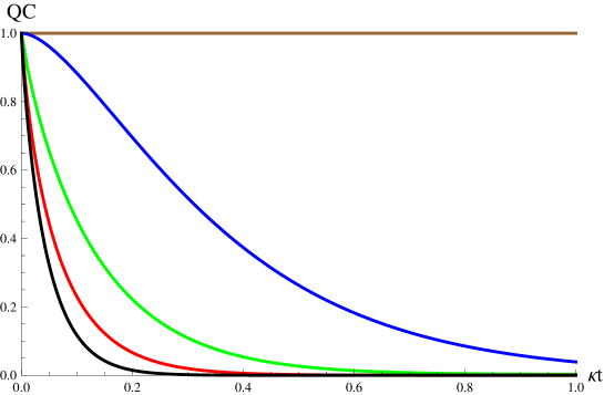
Figure 1: Quantum correlation evaluated by MID and AMID for the three-qubit system with the initial GHZ state as a function of $\kappa t$ transmitted through various noisy channels: Pauli-X by MID (brown line), Pauli-X by AMID (green line), Pauli-Y by MID and AMID (blue line), Pauli-Z by MID and AMID (red line), and isotropic by MID and AMID (black line).

IV Quantumness of correlation for W state

In this section, we determine quantum correlation using MID and AMID for a bipartite state which is initially prepared in the form of W state under various noise channels. The first two qubits belong to party $a$ and the third qubit belongs to party $b$.

In the presence of the Pauli-X noise, the time evolution of the density matrix of W state is given by jung08

$$\rho_{W}^{x}(t)=\frac{1}{16}{\left(\begin{matrix}2\alpha_{2}&0&0&\sqrt{2}\alpha_{2}&0&\sqrt{2}\alpha_{2}&\alpha_{2}&0\\ 0&2\alpha_{1}&\sqrt{2}\alpha_{1}&0&\sqrt{2}\alpha_{1}&0&0&\alpha_{3}\\ 0&\sqrt{2}\alpha_{1}&2\beta_{+}&0&\alpha_{1}&0&0&\sqrt{2}\alpha_{3}\\ \sqrt{2}\alpha_{2}&0&0&2\beta_{-}&0&\alpha_{4}&\sqrt{2}\alpha_{4}&0\\ 0&\sqrt{2}\alpha_{1}&\alpha_{1}&0&2\beta_{+}&0&0&\sqrt{2}\alpha_{3}\\ \sqrt{2}\alpha_{2}&0&0&\alpha_{4}&0&2\beta_{-}&\sqrt{2}\alpha_{4}&0\\ \alpha_{2}&0&0&\sqrt{2}\alpha_{4}&0&\sqrt{2}\alpha_{4}&2\alpha_{4}&0\\ 0&\alpha_{3}&\sqrt{2}\alpha_{3}&0&\sqrt{2}\alpha_{3}&0&0&2\alpha_{3}\end{matrix}\right),}$$ (31)

where

$$\left\{\begin{array}[]{l}\alpha_{1}=1+e^{-2\kappa t}+e^{-4\kappa t}+e^{-6\kappa t},\\ \alpha_{2}=1+e^{-2\kappa t}-e^{-4\kappa t}-e^{-6\kappa t},\\ \alpha_{3}=1-e^{-2\kappa t}-e^{-4\kappa t}+e^{-6\kappa t},\\ \alpha_{4}=1-e^{-2\kappa t}+e^{-4\kappa t}-e^{-6\kappa t},\\ \beta_{\pm}=1\pm e^{-6\kappa t}.\\ \end{array}\right.$$ (37)

The projective measurements are found using the reduced density matrices

$$(\rho_{W}^{x})^{a}=\frac{1}{16}{\left(\begin{matrix}2(\alpha_{1}+\alpha_{2})&0&0&\alpha_{2}+\alpha_{3}\\ 0&2(\beta_{+}+\beta_{-})&\alpha_{1}+\alpha_{4}&0\\ 0&\alpha_{1}+\alpha_{4}&2(\beta_{+}+\beta_{-})&0\\ \alpha_{2}+\alpha_{3}&0&0&2(\alpha_{3}+\alpha_{4})\end{matrix}\right),}\hskip 28.45274pt(\rho_{W}^{x})^{b}=\frac{I}{2},$$ (38)

which results in

$$\left\{\begin{array}[]{l}\Pi_{a,{00}}=\frac{1}{2}(|01\rangle+\langle 10|)(\langle 01|+\langle 10|),\\ \Pi_{a,{11}}=\frac{1}{2}(|01\rangle-\langle 10|)(\langle 01|-\langle 10|),\\ \Pi_{a,{01}}=\frac{1}{2(1+e^{4\kappa t})}\left((1-e^{2\kappa t})^{2}|00\rangle\langle 00|+(1-e^{4\kappa t})|11\rangle\langle 11|\right),\\ \Pi_{a,{10}}=\frac{1}{2(1+e^{4\kappa t})}\left((1+e^{2\kappa t})^{2}|00\rangle\langle 00|-(1-e^{4\kappa t})|11\rangle\langle 11|\right),\\ \end{array}\right.$$ (43)

and $\Pi_{b,i}=|i\rangle\langle i|$. So we have

$$\Pi(\rho_{W}^{x})={\left(\begin{matrix}\gamma_{1}&0&0&0&0&0&\eta_{1}&0\\ 0&\gamma_{2}&0&0&0&0&0&\eta_{2}\\ 0&0&2\beta_{+}&0&\alpha_{1}&0&0&0\\ 0&0&0&2\beta_{-}&0&\alpha_{4}&0&0\\ 0&0&\alpha_{1}&0&2\beta_{+}&0&0&0\\ 0&0&0&\alpha_{4}&0&2\beta_{-}&0&0\\ \eta_{1}&0&0&0&0&0&\gamma_{3}&0\\ 0&\eta_{2}&0&0&0&0&0&\gamma_{4}\end{matrix}\right),}$$ (44)

where

$$\left\{\begin{array}[]{l}\gamma_{1}=\frac{2e^{\kappa t}\cosh(\kappa t)^{2}\sinh(\kappa t)(2-\cosh(2\kappa t)+\cosh(4\kappa t)+\sinh(2\kappa t))}{(1+e^{4\kappa t})^{2}},\\ \gamma_{2}=\frac{1+e^{-6\kappa t}+\frac{8}{(1+e^{4\kappa t})^{2}}+2e^{-3\kappa t}\sinh(\kappa t)}{8},\\ \gamma_{3}=\frac{1-e^{-6\kappa t}+\frac{8}{(1+e^{4\kappa t})^{2}}-2e^{-3\kappa t}\cosh(\kappa t)}{8},\\ \gamma_{4}=\frac{2e^{\kappa t}\cosh(\kappa t)\sinh(\kappa t)^{2}(2+\cosh(2\kappa t)+\cosh(4\kappa t)-\sinh(2\kappa t))}{(1+e^{4\kappa t})^{2}},\\ \eta_{1}=\frac{e^{\kappa t}\sinh(\kappa t)\sinh(2\kappa t)(2+2\sinh(2\kappa t)+\sinh(4\kappa t))}{2(1+e^{4\kappa t})^{2}},\\ \eta_{2}=\frac{e^{\kappa t}\cosh(\kappa t)^{2}\sinh(\kappa t)(2-2\sinh(2\kappa t)+\sinh(4\kappa t))}{(1+e^{4\kappa t})^{2}}.\end{array}\right.$$ (51)

Since $\left[\Pi(\rho_{W}^{x})\right]^{a}=(\rho_{W}^{x})^{a}$ and $\left[\Pi(\rho_{W}^{x})\right]^{b}=(\rho_{W}^{x})^{b}$, the third term of Eq. (6) vanishes and we obtain

$${\cal M}(\rho_{W}^{x})=S(\Pi(\rho_{W}^{x}))-S(\rho_{W}^{x}).$$ (52)

Now, the quantum correlation can be evaluated numerically which is depicted in Fig. 2.

The numerical optimization program for the nine parameters that is inherent in AMID approach gives rise to the following nonclassical correlation

$${\cal A}=\left\{{{{\cal A}(2.23,0,1.1,1.1,0,1.1,1.1,0,1.1,\kappa t),}\atop{{\cal A}(2.2,2.3,2.2,2.2,2.3,2.2,2.2,2.3,2.2,\kappa t),}}\hskip 28.45274pt{{0<\kappa t<0.06,}\atop{\kappa t>0.06,}}\right.$$ (53)

which is depicted in Fig. 2 as a green line.

For the Pauli-Y noise the density matrix reads jung08

$$\rho_{W}^{y}(t)=\frac{1}{16}{\left(\begin{matrix}2\alpha_{2}&0&0&-\sqrt{2}\alpha_{2}&0&-\sqrt{2}\alpha_{2}&-\alpha_{2}&0\\ 0&2\alpha_{1}&\sqrt{2}\alpha_{1}&0&\sqrt{2}\alpha_{1}&0&0&-\alpha_{3}\\ 0&\sqrt{2}\alpha_{1}&2\beta_{+}&0&\alpha_{1}&0&0&-\sqrt{2}\alpha_{3}\\ -\sqrt{2}\alpha_{2}&0&0&2\beta_{-}&0&\alpha_{4}&\sqrt{2}\alpha_{4}&0\\ 0&\sqrt{2}\alpha_{1}&\alpha_{1}&0&2\beta_{+}&0&0&-\sqrt{2}\alpha_{3}\\ -\sqrt{2}\alpha_{2}&0&0&\alpha_{4}&0&2\beta_{-}&\sqrt{2}\alpha_{4}&0\\ -\alpha_{2}&0&0&\sqrt{2}\alpha_{4}&0&\sqrt{2}\alpha_{4}&2\alpha_{4}&0\\ 0&-\alpha_{3}&-\sqrt{2}\alpha_{3}&0&-\sqrt{2}\alpha_{3}&0&0&2\alpha_{3}\end{matrix}\right).}$$ (54)

For this case the results are identical with the previous case. Therefore, the time evolution of ${\cal M}$ for the initial W state under Pauli-Y noise coincides with ${\cal M}(\rho_{W}^{x})$ (see Fig. 2). Also, the evolution of quantum correlation computed by AMID results in

$${\cal A}=\left\{{{{\cal A}(1.57,1.57,1.57,1.57,1.57,1.57,1.57,1.57,1.57,\kappa t)}\atop{{\cal A}(1.57,2.22,1.57,1.57,2.22,1.57,1.57,2.22,1.57,\kappa t)}}\hskip 28.45274pt{{0<\kappa t<0.03}\atop{\kappa t>0.03,}}\right.$$ (55)

which is shown in Fig. 2 as a blue line.

To this end, consider the effects of the Pauli-Z noise on W state jung08

$$\rho_{W}^{z}(t)=\frac{1}{4}{\left(\begin{matrix}0&0&0&0&0&0&0&0\\ 0&2&\sqrt{2}e^{-4\kappa t}&0&\sqrt{2}e^{-4\kappa t}&0&0&0\\ 0&\sqrt{2}e^{-4\kappa t}&1&0&e^{-4\kappa t}&0&0&0\\ 0&0&0&0&0&0&0&0\\ 0&\sqrt{2}e^{-4\kappa t}&e^{-4\kappa t}&0&1&0&0&0\\ 0&0&0&0&0&0&0&0\\ 0&0&0&0&0&0&0&0\\ 0&0&0&0&0&0&0&0\end{matrix}\right).}$$ (56)

So, the reduced density matrices for the subsystems are

$$(\rho_{W}^{z})^{a}=\frac{1}{4}{\left(\begin{matrix}2&0&0&0\\ 0&1&e^{-4\kappa t}&0\\ 0&e^{-4\kappa t}&1&0\\ 0&0&0&0\end{matrix}\right),}\hskip 28.45274pt(\rho_{W}^{z})^{b}=\frac{I}{2},$$ (57)

which result in

$$\left\{\begin{array}[]{l}\Pi_{a,{00}}=|00\rangle\langle 00|,\\ \Pi_{a,{11}}=|11\rangle\langle 11|,\\ \Pi_{a,{01}}=\frac{1}{2}(|01\rangle+\langle 10|)(\langle 01|+\langle 10|),\\ \Pi_{a,{10}}=\frac{1}{2}(|01\rangle-\langle 10|)(\langle 01|-\langle 10|),\\ \end{array}\right.$$ (62)

and $\Pi_{b,i}=|i\rangle\langle i|$. Using the projective measurements we find

$$\Pi(\rho_{W}^{z})=\frac{1}{4}{\left(\begin{matrix}0&0&0&0&0&0&0&0\\ 0&2&0&0&0&0&0&0\\ 0&0&1&0&e^{-4\kappa t}&0&0&0\\ 0&0&0&0&0&0&0&0\\ 0&0&e^{-4\kappa t}&0&1&0&0&0\\ 0&0&0&0&0&0&0&0\\ 0&0&0&0&0&0&0&0\\ 0&0&0&0&0&0&0&0\end{matrix}\right),}$$ (63)

and $\left[\Pi(\rho_{W}^{z})\right]^{a}=(\rho_{W}^{z})^{a}$ and $\left[\Pi(\rho_{W}^{z})\right]^{b}=(\rho_{W}^{z})^{b}$. Therefore, we only need to obtain the following von-Neumann entropies

$$S(\rho_{W}^{z}) = \frac{1}{4}(11+e^{-4\kappa t})-\frac{1}{4}(1-e^{-4\kappa t})\log_{2}(1-e^{-4\kappa t})$$ (64)

$$- \frac{1}{8}[(3+e^{-4\kappa t}-\sqrt{1-2e^{-4\kappa t}+17e^{-8\kappa t}})\log_{2}(3+e^{-4\kappa t}-\sqrt{1-2e^{-4\kappa t}+17e^{-8\kappa t}})$$

$$+ (3+e^{-4\kappa t}+\sqrt{1-2e^{-4\kappa t}+17e^{-8\kappa t}})\log_{2}(3+e^{-4\kappa t}+\sqrt{1-2e^{-4\kappa t}+17e^{-8\kappa t}})],\hskip 19.91684pt$$

and

$$S(\Pi(\rho_{W}^{z}))=\frac{3}{2}-\frac{1}{4}(1-e^{-4\kappa t})\log_{2}(1-e^{-4\kappa t})-\frac{1}{4}(1+e^{-4\kappa t})\log_{2}(1+e^{-4\kappa t}).$$ (65)

Now, the quantum correlation can be found analytically

$${\cal M}(\rho_{W}^{z}) = -\frac{1}{4}(5+e^{-4\kappa t})-\frac{1}{4}(1+e^{-4\kappa t})\log_{2}(1+e^{-4\kappa t})$$ (66)

$$+ \frac{1}{8}[(3+e^{-4\kappa t}-\sqrt{1-2e^{-4\kappa t}+17e^{-8\kappa t}})\log_{2}(3+e^{-4\kappa t}-\sqrt{1-2e^{-4\kappa t}+17e^{-8\kappa t}})$$

$$+ (3+e^{-4\kappa t}+\sqrt{1-2e^{-4\kappa t}+17e^{-8\kappa t}})\log_{2}(3+e^{-4\kappa t}+\sqrt{1-2e^{-4\kappa t}+17e^{-8\kappa t}})].\hskip 19.91684pt$$

Performing the optimization procedure of AMID gives us the same result, namely, ${\cal A}(\theta_{1},\phi_{1},0,\theta_{2},\phi_{2},0,\theta_{3},\phi_{3},0)={\cal M}(\rho_{W}^{z})$. In other words, the infimum value of ${\cal A}$ happens for $\psi_{i}=0$ $(i=1,2,3)$ and arbitrary values of $\phi_{i}$ and $\theta_{i}$.

For the last case, consider the isotropic noise. The corresponding density matrix reads jung08

$$\rho_{W}^{d}(t)=\frac{1}{8}{\left(\begin{matrix}\tilde{\alpha}_{2}&0&0&0&0&0&0&0\\ 0&\tilde{\alpha}_{1}&\sqrt{2}\tilde{\gamma}_{+}&0&\sqrt{2}\tilde{\gamma}_{+}&0&0&0\\ 0&\sqrt{2}\tilde{\gamma}_{+}&\tilde{\beta}_{+}&0&\tilde{\gamma}_{+}&0&0&0\\ 0&0&0&\tilde{\beta}_{-}&0&\tilde{\gamma}_{-}&\sqrt{2}\tilde{\gamma}_{-}&0\\ 0&\sqrt{2}\tilde{\gamma}_{+}&\tilde{\gamma}_{+}&0&\tilde{\beta}_{+}&0&0&0\\ 0&0&0&\tilde{\gamma}_{-}&0&\tilde{\beta}_{-}&\sqrt{2}\tilde{\gamma}_{-}&0\\ 0&0&0&\sqrt{2}\tilde{\gamma}_{-}&0&\sqrt{2}\tilde{\gamma}_{-}&\tilde{\alpha}_{4}&0\\ 0&0&0&0&0&0&0&\tilde{\alpha}_{3}\end{matrix}\right),}$$ (67)

where

$$\left\{\begin{array}[]{l}\tilde{\alpha}_{1}=1+e^{-4\kappa t}+e^{-8\kappa t}+e^{-12\kappa t},\\ \tilde{\alpha}_{2}=1+e^{-4\kappa t}-e^{-8\kappa t}-e^{-12\kappa t},\\ \tilde{\alpha}_{3}=1-e^{-4\kappa t}-e^{-8\kappa t}+e^{-12\kappa t},\\ \tilde{\alpha}_{4}=1-e^{-4\kappa t}+e^{-8\kappa t}-e^{-12\kappa t},\\ \tilde{\gamma}_{\pm}=1\pm e^{-6\kappa t}.\\ \end{array}\right.$$ (73)

The reduced density matrices are given by

$$(\rho_{W}^{d})^{a}=\frac{1}{8}{\left(\begin{matrix}\tilde{\alpha_{1}}+\tilde{\alpha_{2}}&0&0&0\\ 0&\tilde{\beta_{-}}+\tilde{\beta_{+}}&\tilde{\gamma_{-}}+\tilde{\gamma_{+}}&0\\ 0&\tilde{\gamma_{-}}+\tilde{\gamma_{+}}&\tilde{\beta_{-}}+\tilde{\beta_{+}}&0\\ 0&0&0&\tilde{\alpha_{3}}+\tilde{\alpha_{4}}\end{matrix}\right),}\hskip 14.22636pt(\rho_{W}^{d})^{b}=\frac{1}{8}{\left(\begin{matrix}\tilde{\beta_{+}}+\tilde{\alpha_{2}}+\tilde{\alpha_{4}}&0\\ 0&\tilde{\beta_{-}}+\tilde{\alpha_{1}}+\tilde{\alpha_{3}}\end{matrix}\right),}\hskip 14.22636pt$$ (74)

and

$$\Pi(\rho_{W}^{d})=\frac{1}{8}{\left(\begin{matrix}\tilde{\alpha_{2}}&0&0&0&0&0&0&0\\ 0&\tilde{\alpha_{1}}&0&0&0&0&0&0\\ 0&0&\tilde{\beta_{+}}&0&\tilde{\gamma_{+}}&0&0&0\\ 0&0&0&\tilde{\beta_{-}}&0&\tilde{\gamma_{-}}&0&0\\ 0&0&\tilde{\gamma_{+}}&0&\tilde{\beta_{+}}&0&0&0\\ 0&0&0&\tilde{\gamma_{-}}&0&\tilde{\beta_{-}}&0&0\\ 0&0&0&0&0&0&\tilde{\alpha_{4}}&0\\ 0&0&0&0&0&0&0&\tilde{\alpha_{3}}\end{matrix}\right)}.$$ (75)

Tracing out the first two qubits and the third qubit leads to $\left[\Pi(\rho_{W}^{d})\right]^{a}=(\rho_{W}^{d})^{a}$ and $\left[\Pi(\rho_{W}^{d})\right]^{b}=(\rho_{W}^{d})^{b}$ which results in $S((\rho_{W}^{d})^{a})=S(\Pi(\rho_{W}^{d})^{a})$ and $S((\rho_{W}^{d})^{b})=S(\Pi(\rho_{W}^{d})^{b})$. Thus, using the von-Neumann entropies

$$S(\rho_{W}^{d}) = \frac{1}{2}(7+e^{-8\kappa t})-\frac{1}{8}[\tilde{\alpha}_{2}\log_{2}\tilde{\alpha}_{2}+\tilde{\alpha}_{3}\log_{2}\tilde{\alpha}_{3}$$ (77)

$$+ (\tilde{\beta}_{+}-\tilde{\gamma}_{+})\log_{2}(\tilde{\beta}_{+}-\tilde{\gamma}_{+})+(\tilde{\beta}_{-}-\tilde{\gamma}_{-})\log_{2}(\tilde{\beta}_{-}-\tilde{\gamma}_{-})]$$

$$- \frac{1}{16}[(\tilde{\beta}_{+}+\tilde{\gamma}_{+}+\tilde{\alpha}_{1}+\sqrt{\tilde{\beta}_{+}^{2}+2\tilde{\beta}_{+}\tilde{\gamma}_{+}+17\tilde{\gamma}_{+}^{2}-2\tilde{\beta}_{+}\tilde{\alpha}_{1}-2\tilde{\gamma}_{+}\tilde{\alpha}_{1}+\tilde{\alpha}_{1}^{2}})$$

$$\log_{2}(\tilde{\beta}_{+}+\tilde{\gamma}_{+}+\tilde{\alpha}_{1}+\sqrt{\tilde{\beta}_{+}^{2}+2\tilde{\beta}_{+}\tilde{\gamma}_{+}+17\tilde{\gamma}_{+}^{2}-2\tilde{\beta}_{+}\tilde{\alpha}_{1}-2\tilde{\gamma}_{+}\tilde{\alpha}_{1}+\tilde{\alpha}_{1}^{2}})$$

$$+ (\tilde{\beta}_{+}+\tilde{\gamma}_{+}+\tilde{\alpha}_{1}-\sqrt{\tilde{\beta}_{+}^{2}+2\tilde{\beta}_{+}\tilde{\gamma}_{+}+17\tilde{\gamma}_{+}^{2}-2\tilde{\beta}_{+}\tilde{\alpha}_{1}-2\tilde{\gamma}_{+}\tilde{\alpha}_{1}+\tilde{\alpha}_{1}^{2}})$$

$$\log_{2}(\tilde{\beta}_{+}+\tilde{\gamma}_{+}+\tilde{\alpha}_{1}-\sqrt{\tilde{\beta}_{+}^{2}+2\tilde{\beta}_{+}\tilde{\gamma}_{+}+17\tilde{\gamma}_{+}^{2}-2\tilde{\beta}_{+}\tilde{\alpha}_{1}-2\tilde{\gamma}_{+}\tilde{\alpha}_{1}+\tilde{\alpha}_{1}^{2}})$$

$$+ (\tilde{\beta}_{-}+\tilde{\gamma}_{-}+\tilde{\alpha}_{4}+\sqrt{\tilde{\beta}_{-}^{2}+2\tilde{\beta}_{-}\tilde{\gamma}_{-}+17\tilde{\gamma}_{-}^{2}-2\tilde{\beta}_{-}\tilde{\alpha}_{4}-2\tilde{\gamma}_{-}\tilde{\alpha}_{4}+\tilde{\alpha}_{4}^{2}})$$

$$\log_{2}(\tilde{\beta}_{-}+\tilde{\gamma}_{-}+\tilde{\alpha}_{4}+\sqrt{\tilde{\beta}_{-}^{2}+2\tilde{\beta}_{-}\tilde{\gamma}_{-}+17\tilde{\gamma}_{-}^{2}-2\tilde{\beta}_{-}\tilde{\alpha}_{4}-2\tilde{\gamma}_{-}\tilde{\alpha}_{4}+\tilde{\alpha}_{4}^{2}})$$

$$+ (\tilde{\beta}_{-}+\tilde{\gamma}_{-}+\tilde{\alpha}_{4}-\sqrt{\tilde{\beta}_{-}^{2}+2\tilde{\beta}_{-}\tilde{\gamma}_{-}+17\tilde{\gamma}_{-}^{2}-2\tilde{\beta}_{-}\tilde{\alpha}_{4}-2\tilde{\gamma}_{-}\tilde{\alpha}_{4}+\tilde{\alpha}_{4}^{2}})$$

$$\log_{2}(\tilde{\beta}_{-}+\tilde{\gamma}_{-}+\tilde{\alpha}_{4}-\sqrt{\tilde{\beta}_{-}^{2}+2\tilde{\beta}_{-}\tilde{\gamma}_{-}+17\tilde{\gamma}_{-}^{2}-2\tilde{\beta}_{-}\tilde{\alpha}_{4}-2\tilde{\gamma}_{-}\tilde{\alpha}_{4}+\tilde{\alpha}_{4}^{2}})],\hskip 19.91684pt$$

and

$$S(\Pi(\rho_{W}^{d})) = 3-\frac{1}{8}[\tilde{\alpha}_{1}\log_{2}\tilde{\alpha}_{1}+\tilde{\alpha}_{2}\log_{2}\tilde{\alpha}_{2}+\tilde{\alpha}_{3}\log_{2}\tilde{\alpha}_{3}+\tilde{\alpha}_{4}\log_{2}\tilde{\alpha}_{4}$$ (78)

$$+ (\tilde{\beta}_{+}+\tilde{\gamma}_{+})\log_{2}(\tilde{\beta}_{+}+\tilde{\gamma}_{+})+(\tilde{\beta}_{+}-\tilde{\gamma}_{+})\log_{2}(\tilde{\beta}_{+}-\tilde{\gamma}_{+})$$

$$+ (\tilde{\beta}_{-}+\tilde{\gamma}_{-})\log_{2}(\tilde{\beta}_{-}+\tilde{\gamma}_{-})+(\tilde{\beta}_{-}-\tilde{\gamma}_{-})\log_{2}(\tilde{\beta}_{-}-\tilde{\gamma}_{-})],$$

the quantum correlation reads

$${\cal M}(\rho_{W}^{d}) = -\frac{(1+e^{-8\kappa t})}{2}-\frac{1}{8}[\tilde{\alpha}_{1}\log_{2}\tilde{\alpha}_{1}+\tilde{\alpha}_{4}\log_{2}\tilde{\alpha}_{4}$$ (80)

$$+ (\tilde{\beta}_{+}+\tilde{\gamma}_{+})\log_{2}(\tilde{\beta}_{+}+\tilde{\gamma}_{+})+(\tilde{\beta}_{-}+\tilde{\gamma}_{-})\log_{2}(\tilde{\beta}_{-}+\tilde{\gamma}_{-})]$$

$$+ \frac{1}{16}[(\tilde{\beta}_{+}+\tilde{\gamma}_{+}+\tilde{\alpha}_{1}+\sqrt{\tilde{\beta}_{+}^{2}+2\tilde{\beta}_{+}\tilde{\gamma}_{+}+17\tilde{\gamma}_{+}^{2}-2\tilde{\beta}_{+}\tilde{\alpha}_{1}-2\tilde{\gamma}_{+}\tilde{\alpha}_{1}+\tilde{\alpha}_{1}^{2}})$$

$$\log_{2}(\tilde{\beta}_{+}+\tilde{\gamma}_{+}+\tilde{\alpha}_{1}+\sqrt{\tilde{\beta}_{+}^{2}+2\tilde{\beta}_{+}\tilde{\gamma}_{+}+17\tilde{\gamma}_{+}^{2}-2\tilde{\beta}_{+}\tilde{\alpha}_{1}-2\tilde{\gamma}_{+}\tilde{\alpha}_{1}+\tilde{\alpha}_{1}^{2}})$$

$$+ (\tilde{\beta}_{+}+\tilde{\gamma}_{+}+\tilde{\alpha}_{1}-\sqrt{\tilde{\beta}_{+}^{2}+2\tilde{\beta}_{+}\tilde{\gamma}_{+}+17\tilde{\gamma}_{+}^{2}-2\tilde{\beta}_{+}\tilde{\alpha}_{1}-2\tilde{\gamma}_{+}\tilde{\alpha}_{1}+\tilde{\alpha}_{1}^{2}})$$

$$\log_{2}(\tilde{\beta}_{+}+\tilde{\gamma}_{+}+\tilde{\alpha}_{1}-\sqrt{\tilde{\beta}_{+}^{2}+2\tilde{\beta}_{+}\tilde{\gamma}_{+}+17\tilde{\gamma}_{+}^{2}-2\tilde{\beta}_{+}\tilde{\alpha}_{1}-2\tilde{\gamma}_{+}\tilde{\alpha}_{1}+\tilde{\alpha}_{1}^{2}})$$

$$+ (\tilde{\beta}_{-}+\tilde{\gamma}_{-}+\tilde{\alpha}_{4}+\sqrt{\tilde{\beta}_{-}^{2}+2\tilde{\beta}_{-}\tilde{\gamma}_{-}+17\tilde{\gamma}_{-}^{2}-2\tilde{\beta}_{-}\tilde{\alpha}_{4}-2\tilde{\gamma}_{-}\tilde{\alpha}_{4}+\tilde{\alpha}_{4}^{2}})$$

$$\log_{2}(\tilde{\beta}_{-}+\tilde{\gamma}_{-}+\tilde{\alpha}_{4}+\sqrt{\tilde{\beta}_{-}^{2}+2\tilde{\beta}_{-}\tilde{\gamma}_{-}+17\tilde{\gamma}_{-}^{2}-2\tilde{\beta}_{-}\tilde{\alpha}_{4}-2\tilde{\gamma}_{-}\tilde{\alpha}_{4}+\tilde{\alpha}_{4}^{2}})$$

$$+ (\tilde{\beta}_{-}+\tilde{\gamma}_{-}+\tilde{\alpha}_{4}-\sqrt{\tilde{\beta}_{-}^{2}+2\tilde{\beta}_{-}\tilde{\gamma}_{-}+17\tilde{\gamma}_{-}^{2}-2\tilde{\beta}_{-}\tilde{\alpha}_{4}-2\tilde{\gamma}_{-}\tilde{\alpha}_{4}+\tilde{\alpha}_{4}^{2}})$$

$$\log_{2}(\tilde{\beta}_{-}+\tilde{\gamma}_{-}+\tilde{\alpha}_{4}-\sqrt{\tilde{\beta}_{-}^{2}+2\tilde{\beta}_{-}\tilde{\gamma}_{-}+17\tilde{\gamma}_{-}^{2}-2\tilde{\beta}_{-}\tilde{\alpha}_{4}-2\tilde{\gamma}_{-}\tilde{\alpha}_{4}+\tilde{\alpha}_{4}^{2}})].\hskip 28.45274pt$$

Quantum correlation obtained by AMID for this case is ${\cal A}(\theta_{1},\phi_{1},0,\theta_{2},\phi_{2},0,\theta_{3},\phi_{3},0)$ coincides with the one obtained by MID (black line in Fig. 2). The MID and AMID for the three-qubit initial W state under various noisy channels are depicted in Fig. 2. As it can be seen from the figure, the quantum correlations obtained by MID for two cases of Pauli-X and -Y channels are overestimated with respect to ones obtained by AMID. Notice that, for the initial W state our results do not agree with the results obtained by quantum discord which is due to the different choices of the projective measurements mah12 .

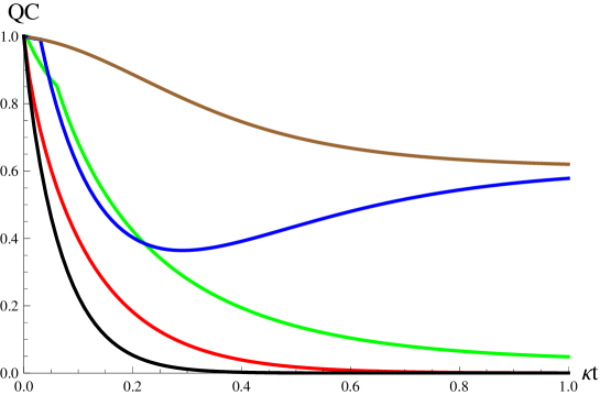
Figure 2: Quantum correlation evaluated by MID and AMID for the three-qubit system with the initial W state as a function of $\kappa t$ transmitted through various noisy channels: Pauli-X and Pauli-Y by MID (brown line), Pauli-X by AMID (green line), Pauli-Y by AMID (blue line), Pauli-Z by MID and AMID (red line), and isotropic by MID and AMID (black line).

V Conclusions

In this paper, we have studied quantum correlations for the initial GHZ and W states in the presence of various noisy channels using the measurement-induced disturbance and its ameliorated version. We considered the solutions of the Lindblad equation where the noises are represented by the Pauli-X, Pauli-Y, Pauli-Z and isotropic operators. This idea is based on the fact that the classical measurements can be performed without disturbance. However, measurements usually disturb the system in the quantum description and this disturbance can be used to determine the quantumness of correlations. In the absence of noise, quantum correlations of GHZ and W states are equal to unity, namely the half of the total correlation which is expected for a pure state. After turning on noises, quantum correlation decreases for all noises. For the case of the initial W state under Pauli-Y noisy channel (unlike GHZ state that its corresponding quantum correlation vanishes for large $\kappa t$), ${\cal A}(\rho_{W}^{y})$ tends to $0.58$ as $\kappa t$ goes to infinity. In comparison, our results showed that in the MID approach the W state is more robust than GHZ state under noisy channels except Pauli-X channel. This result is also valid for the AMID scenario except Pauli-Y channel for $0<\kappa t<0.4$. Moreover, the obtained results for ${\cal M}(\rho)$ coincided with those of quantum discord just for the initial GHZ state. Indeed, both the quantum discord and MID overestimate quantum correlations of states with respect to AMID in agreement with Ref. girolami11 .

References

• (1) M.A. Nielsen and I.L. Chuang, Quantum Computation and Quantum Information (Cambridge University Press, Cambridge, England, 2000).
• (2) C.H. Bennett, D.P. DiVincenzo, C.A. Fuchs, T. Mor, E. Rains, P.W. Shore, J.A. Smolin, and W.K. Wootters, Phys. Rev. A 59, 1070 (1999).
• (3) S.L. Braunstein, C.M. Caves, R. Jozsa, N. Linden, S. Popescu, and R. Schack, Phys. Rev. Lett. 83, 1054 (1999).
• (4) D.A. Meyer, Phys. Rev. Lett. 85, 2014 (2000).
• (5) E. Biham, G. Brassard, D. Kenigsberg, and T. Mor, Theor. Comput. Sci. 320, 15 (2004).
• (6) A. Datta, S.T. Flammia, and C.M. Caves, Phys. Rev. A 72, 042316 (2005); A. Datta and G. Vidal, ibid. 75, 042310 (2007).
• (7) H. Ollivier and W.H. Zurek, Phys. Rev. Lett. 88, 017901 (2001).
• (8) A.K. Rajagopal and R.W. Rendell, Phys. Rev. A 66, 022104 (2002).
• (9) M. Horodecki, P. Horodecki, R. Horodecki, J. Oppenheim, A. Sen(De), U. Sen, and B. Synak-Radtke, Phys. Rev. A 71, 062307 (2005).
• (10) I. Devetak, Phys. Rev. A 71, 062303 (2005).
• (11) A.R. Usha Devi and A.K. Rajagopal, Phys. Rev. Lett. 100, 140502 (2008).
• (12) K. Modi, T. Paterek, W. Son, V. Vedral, and M. Williamson, Phys. Rev. Lett. 104, 080501 (2010).
• (13) A. Shabani and Daniel A. Lidar, Phys. Rev. Lett. 102, 100402 (2009).
• (14) C.C. Rulli and M.S. Sarandy, Phys. Rev. A 84, 042109 (2011).
• (15) P. Giorda, M. Allegra, Matteo G.A. Paris, Phys. Rev. A 86, 052328 (2012).
• (16) A.F. Terzis, P. Androvitsaneas, and E. Paspalakis, Quant. Inf. Proc. 11, 1931 (2012).
• (17) J.P.G. Pinto, G. Karpat, and F.F. Fanchini, Phys. Rev. A 88, 034304 (2013).
• (18) D. Girolami and G. Adesso, Phys. Rev. A 83, 052108 (2011).
• (19) S. Luo, Phys. Rev. A 77, 042303 (2008).
• (20) M. Ali, A.R.P. Rau, and G. Alber, Phys. Rev. A 81, 042105 (2010); M. Ali, A.R.P. Rau, and G. Alber, ibid. 82, 069902(E) (2010).
• (21) X.-M. Lu, J. Ma, Z. Xi, and X. Wang, Phys. Rev. A 83, 012327 (2011).
• (22) Q. Chen, C. Zhang, S. Yu, X.X. Yi, and C.H. Oh, Phys. Rev. A 84, 042313 (2011).
• (23) S. Luo, Phys. Rev. A 77, 022301 (2008).
• (24) D. Girolami, M. Paternostro, and G. Adesso, J. Phys. A 44, 352002 (2011).
• (25) D.M. Greenberger, M.A. Horne, and A. Zeilinger, Bells Theorem, Quantum Theory, and Conceptions of the Universe, edited by M. Kafatos (Kluwer, Dordrecht, 1989) pp. 69.
• (26) W. Dur, G. Vidal, and J.I. Cirac, Phys. Rev. A 62, 062314 (2000).
• (27) P. Agrawal and A. Pati, Phys. Rev. A 74, 062320 (2006).
• (28) G. Lindblad, Commun. Math. Phys. 48, 119 (1976).
• (29) E. Jung, M.-R. Hwang, Y.H. Ju, M.-S. Kim, S.-K. Yoo, H. Kim, D. Park, J.-W. Son, S. Tamaryan, and S.-K. Cha, Phys. Rev. A 78, 012312 (2008).
• (30) P. Espoukeh and P. Pedram, Quant. Inf. Proc. 13, 1789 (2014), arXiv:1403.1147.
• (31) M. Mahdian, R. Yousefjani and S. Salimi, Eur. Phys. J. D 66, 133 (2012).