Calculation of a power price equilibrium

Abstract

In this paper we propose a tractable quadratic programming formulation for calculating the equilibrium term structure of electricity prices. We rely on a theoretical model described in [21], but extend it so that it reflects actually traded electricity contracts, transaction costs and liquidity considerations. Our numerical simulations examine the properties of the term structure and its dependence on various parameters of the model. The proposed quadratic programming formulation is applied to calculate the equilibrium term structure of electricity prices in the UK power grid consisting of a few hundred power plants. The impact of ramp up and ramp down constraints are also studied.

1 Introduction

Since the deregulation of the electricity markets in the 1990s, the modeling of electricity prices has attracted a lot of attention. A first approach, nowadays called the non-structural approach, attempted to model electricity prices by using the standard techniques that had already been developed for modeling the prices of other financial securities. The seminal paper [18] studied the suitability of one and multi-factor Ornstein-Uhlenbeck processes to model the spot price. As pointed out in this work, Gaussian distributions alone can not be used for modeling spikes, and thus the Ornstein-Uhlenbeck process was combined with a pure jump-process in [15]. An extension to more general Levy processes has been described in [19]. However, as argued in [5], such approaches cannot be directly used for pricing electricity derivatives, because they neglect the non-storable nature of power. They all rely on the non-arbitrage principle and thus implicitly assume that a buy-and-hold strategy is possible. Such an assumption is clearly not realistic for the electricity market. Thus, other models that try to capture some of the physical properties of electricity have been proposed.

The seminal work [4] uses the supply and demand stack to calculate the electricity prices. The model was extended in [16] and [9], where the supply stack was modeled as a function of the underlying fuels (e.g. gas, coal, oil…) used to produce the electricity. A closed form solution for electricity forward contracts, and for spark and dark spread options was derived. These models capture some of the physical properties of the power markets and in the literature they are referred to as structural approaches. However, as argued in [20], models that include the ramp up/down constraints of power plants and long term contracts are needed in order to understand and prevent catastrophic events and market manipulation as happened in California in 2001.

This is the motivation behind a third, game theoretic approach, that models the physical properties and decisions of market participants more closely. The seminal work in this line of research was produced by [6], where a dependency between a forward and a spot price in a two-stage market is studied. The market consists of one producer and one consumer, who each aim to optimize a mean-variance utility function. [10] used this work to study the impact of derivatives in the power market. [8], and [7] have extended it to a multi-stage setting and derived a formula for a dynamic equilibrium. The mean-variance objective function was replaced by a general convex risk measure in [13]. [21] extended the work of [7] to a setting with more than one producer and consumer, who optimize their mean-variance objective functions. In contrast to other game theoretic models, capacity and ramp up/down constraints of power plants are included. By modeling the profit of power plants as a difference between the power price and fuel costs together with emissions obligations, this work also incorporates ideas from the structural approach. As in [11] and in [12], the model is consistent with observable fuel and emission prices. However, [21] focuses only on the description of the model and on the proof of the existence and uniqueness of the solution. In this paper, we extend the model of [21] to include transaction costs, liquidity constraints and actually traded electricity contracts as well as propose a tractable quadratic programming formulation to solve it numerically. The numerical results show the dependence of the term structure of electricity prices on various parameters of the model. Moreover, the algorithm is applied to a realistic setting by incorporating the entire UK power grid, consisting of a few hundred power plants.

From our model, it might not be immediately clear why market participants do not execute all trades at the beginning of the planning horizon. One reason for spreading out the trading activity is the availability of contracts and their liquidity: contracts with a delivery far into the future are much less liquid than, for example, day ahead contracts. Liquidity is included in our model through increased costs of trading (see Subsection 5.3). Another reason are delayed cash flows: when trading is done through future contracts, some players might be interested in entering into a position later and thus delay the associated cash flows. In this paper we mainly postulate the use of forward contracts. A simple extension to future contracts (assuming a constant interest rate) is presented in Subsection 5.1. A third reason for delayed trading is the exploitation of a trend-following effect in the term structure: due to risk aversion of most players, the term structure of forward or future contracts with fixed delivery date is usually slightly upward sloping. A fourth reason are transaction costs: when large trades, such as hedging of a whole power plant, must be executed, they must be spread over a longer period of time to decrease transaction costs and market impact.

Our paper is organized as follows: To keep the paper self contained, we introduce the main components of the term structure power price model presented in [21] in Section 3. A quadratic programming formulation that can be used to calculate the price equilibrium is described in Section 4. In Section 5 we continue with various realistic extensions of the model. In Section 6, we illustrate the forecasting power of our model through numerical experiments. In the first part of this section we study the term structure of electricity prices on a simple example. In the second part we calculate the equilibrium electricity price while modeling the entire system of UK power plants. We conclude the paper in Section 7.

2 Organization of the UK Electricity Market

Electricity supply and demand must match continuously in real-time, which makes electricity grids very difficult to manage. At a high level scale, the UK electricity market can be divided into two different modes of operation: The first mode deals with electricity contracts with more distant delivery periods (ranging from seasons to one hour). The second mode is performed by the system operator (in the UK called the National Grid) responsible for the micromanagement of the grid in the last hour before the delivery of electricity.

In the first mode electricity is traded through forward or future contracts. Forward contracts start to be traded up to four years before delivery. This period is usually referred to as a liquid period. In the beginning of a liquid period only seasonal contracts are available. Seasonal forward contracts are agreements between a buyer and a seller that the seller will deliver a certain fixed amount of electricity in every half hour during the season of interest at a price decided upon today. As we get closer to the delivery, electricity contracts with greater granularity appear. We can find quarterly, monthly, weekly, daily, and intra day contracts. Intra day contracts can cover blocks of twelve hours, four hours, two hours, one hour and the smallest granularity is half an hour (see the APX power exchange for details). Furthermore, various combinations of the above, such as month-ahead peak contracts, which cover all half hours between 7am and 7pm in the following month, are traded. One could use such contracts to hedge the production of a solar power plant, for example. As we can see there exist a huge variety of different contracts. Some of them are traded through an exchange, while others are traded over-the-counter (OTC). In the Wholesale Market Report from the Energy UK, we can see that a large majority of contracts is traded OTC. When choosing the right contract to trade, one also has to take into consideration liquidity and transaction costs. The Wholesale Market Reports from Energy UK show that contracts with a delivery after two or more years tend to be very illiquid. Baseload contracts are much more liquid than peak (i.e. 7am to 7pm) or off-peak (i.e. 7pm to 7am) contracts. The bid-ask spread for different types of contracts between years 2008 and 2011 is available in the Ofgem report. Besides trading electricity through future and forward contracts, a significant amount of electricity is also traded through day-ahead auctions. According to the Wholesale Market Report from Energy UK, roughly between 15% and 20% of power is traded through day-ahead auctions offered by APX and N2EX. Since the auctions are not explicitly included in our model, we will not study them in further detail. An optimal bidding strategy for the auction market is discussed in [2] and [3].

One hour before the delivery, at the event called a Gate Closure, trading of future and forward contracts ceases. This is when the system operator takes over the management of the power grid. All market participants inform the system operator about their positions in future and forward contracts. They also submit their bids and offers. A bid is a pair of volume and a price which tells the system operator at what price a producer can increase production. Similarly, the offer tell the system operator what compensation the producer is willing to accept from the operator if asked to decrease the production. Consumers with a flexible consumption also submit bids and offers. Equipped with this information the system operator first compares the demand forecast with the submitted number of traded contracts and adjusts the difference by accepting some of the bids or offers. While doing so, the system operator must also take into account the capacity constraints of the transmission lines in the network. After the delivery of electricity, the system operator compares the actual physical production/consumption of electricity by each market participant with the contracted volumes adjusted by the accepted bids and offers and calculates the imbalance volume as the difference between the two. If the imbalance volume helped the system operator match supply and demand, then a fair, market index price, is used to calculate the imbalance cash flow to/from each player. On the other hand, if the imbalance volume hampered the system operator in matching supply and demand, then a worse price is applied to calculate the cash flow. Roughly speaking, this price is calculated as the average of the most expensive 500 MWh of accepted bids or offers adjusted by transmission losses.

The two modes of operation described above are very different. The first mode of operation can be considered as a competitive market without a central agent, while the second is controlled by the system operator who is responsible for matching the electricity supply and demand by choosing the cheapest actions. The first mode of operation can be seen as relatively independent of the second mode and thus, this work focuses on the first mode of the operation only. A coupling of both modes is something that we would like to investigate in the future.

3 Problem description

In this section we provide a detailed description of a model that we use for the purpose of modeling the term structure of electricity prices. The model belongs to a class of game theoretic equilibrium models. Market participants are divided into consumers and producers. A set of consumers is denoted by $C$ and has cardinality $0<\left|C\right|<\infty$. Similarly, a set of producers is denoted by $P$ and has cardinality $0<\left|P\right|<\infty$. Each producer owns a portfolio of power plants that can have different characteristics such as capacity, ramp-up and ramp-down constraints, efficiency, and fuel type. The set of all fuel types is denoted by $L$. Sets $R^{p,l}$ denote all power plants owned by producer $p\in P$ that run on fuel $l\in L$. A set $R^{p,l}$ may be empty since each producer typically does not own all possible types of power plants. Moreover, this allows us to include non physical traders such as banks or speculators, who do not own any electricity generation facilities and are without a physical demand for electricity, as producers $p\in P$ with $R^{p,l}=\left\{\right\}$ for all $l\in L$.

As we will see in Subsection 3.4, it is useful to introduce another player named the hypothetical market agent besides producers and consumers. The hypothetical market agent plays the role of the electricity market and ensures that the term structure of the electricity price is such that the market clearing condition is satisfied for all electricity forward contracts.

We are interested in delivery times $T_{j}$, $j\in J=\left\{1,...,T^{\prime}\right\}$, where power for each delivery time $T_{j}$ can be traded through numerous forward contracts at times $t_{i}$, $i\in I_{j}$. The electricity price at time $t_{i}$ for delivery at time $T_{j}$ is denoted by $\Pi\left(t_{i},T_{j}\right)$. Since contracts with trading time later than delivery time do not exist, we require $t_{\max\left\{I_{j}\right\}}=T_{j}$ for all $j\in J$. The number of all forward contracts, i.e. $\sum_{j\in J}\left|I_{j}\right|$, is denoted by $N$. Uncertainty is modeled by a filtered probability space $\left(\Omega,\mathcal{F},\mathbb{F}=\left\{\mathcal{F}_{t},t\in I\right\},\mathbb{P}\right)$, where $I=\cup_{j\in J}I_{j}$. The $\sigma$-algebra $\mathcal{F}_{t}$ represents information available at time $t$.

The exogenous variables that appear in our model are (a) aggregate power demand $D\left(T_{j}\right)$ for each delivery period $j\in J$, (b) prices of fuel forward contracts $G_{l}\left(t_{i},T_{j}\right)$ for each fuel $l\in L$, delivery period $j\in J$, and trading period $i\in I_{j}$, and (c) prices of emissions forward contracts $G_{em}\left(t_{i},T_{j}\right)$, $j\in J$, $i\in I_{j}$. Electricity prices and all exogenous variables are assumed to be adapted to the filtration $\left\{\mathcal{F}_{t}\right\}_{t\in I}$ and have finite second moments.

Let $v_{k}\in\mathbb{R}^{n_{k}}$, $n_{k}\in\mathbb{N}$, $k\in K$, and $K=\left\{1,...,\left|K\right|\right\}$ be given vectors. For convenience, we define a vector concatenation operator as

$$\left|\right|_{k\in K}v_{k}=\left[v_{1}^{\top},...,v_{\left|K\right|}^{\top}\right]^{\top}.$$

3.1 Producer

Each producer $p\in P$ participates in the electricity, fuel, and emission markets. Forward as well as spot contracts are available on all markets. Electricity prices, fuel prices, and emission prices are denoted by $\Pi\left(t_{i},T_{j}\right)$, $G_{l}\left(t_{i},T_{j}\right)$ where $l\in L$, and $G_{em}\left(t_{i},T_{j}\right)$, respectively. To simplify the notation, we introduce

• electricity price vectors $\Pi\left(T_{j}\right)=\left|\right|_{i\in I_{j}}\Pi\left(t_{i},T_{j}\right)$, and $\Pi=\left|\right|_{j\in J}e^{-\hat{r}T_{j}}\Pi\left(T_{j}\right)$, where $\hat{r}\in\mathbb{R}$ is a constant interest rate,

• fuel price vectors $G\left(t_{i},T_{j}\right)=\left|\right|_{l\in L}G_{l}\left(t_{i},T_{j}\right)$, $G\left(T_{j}\right)=\left|\right|_{i\in I_{j}}G\left(t_{i},T_{j}\right)$, and $G=\left|\right|_{j\in J}e^{-\hat{r}T_{j}}G\left(T_{j}\right)$,

• emission price vector $G_{em}\left(T_{j}\right)=\left|\right|_{i\in I_{j}}G_{em}\left(t_{i},T_{j}\right)$, and $G_{em}=\left|\right|_{j\in J}e^{-\hat{r}T_{j}}G_{em}\left(T_{j}\right)$.

A producer may participate in the market by buying and selling forward and spot contracts. The number of electricity forward contracts that producer $p\in P$ buys at trading time $t_{i}$, $i\in I_{j}$ for delivery at time $T_{j}$, $j\in J$ is denoted by $V_{p}\left(t_{i},T_{j}\right)$. Similarly, the number of fuel and emission forward contracts that producer $p\in P$ buys at trading time $t_{i}$, $i\in I_{j}$ for delivery at time $T_{j}$, $j\in J$ is denoted by $F_{p,l}\left(t_{i},T_{j}\right)$, $l\in L$ and $O_{p}\left(t_{i},T_{j}\right)$, respectively. Producers own a generally non-empty portfolio of power plants. The actual production of electricity from power plant $r\in R^{p,l}$ at delivery time $T_{j}$, $j\in J$ is denoted by $W_{p,l,r}\left(T_{j}\right)$.

The notation is greatly simplified if the decision variables are concatenated into

• electricity trading vectors $V_{p}\left(T_{j}\right)=\left|\right|_{i\in I_{j}}V_{p}\left(t_{i},T_{j}\right)$ and $V_{p}=\left|\right|_{j\in J}V_{p}\left(T_{j}\right)$,

• fuel trading vectors $F_{p}\left(t_{i},T_{j}\right)=\left|\right|_{l\in L}F_{p,l}\left(t_{i},T_{j}\right)$, $F_{p}\left(T_{j}\right)=\left|\right|_{i\in I_{j}}F_{p}\left(t_{i},T_{j}\right)$, and $F_{p}=\left|\right|_{j\in J}F_{p}\left(T_{j}\right)$,

• emission trading vectors $O_{p}\left(T_{j}\right)=\left|\right|_{i\in I_{j}}O_{p}\left(t_{i},T_{j}\right)$ and $O_{p}=\left|\right|_{j\in J}O_{p}\left(T_{j}\right)$,

• electricity production vectors $W_{p,l}\left(T_{j}\right)=\left|\right|_{r\in R^{p,l}}W_{p,l,r}\left(T_{j}\right)$, $W_{p}\left(T_{j}\right)=\left|\right|_{l\in L}W_{p,l}\left(T_{j}\right)$, and $W_{p}=\left|\right|_{j\in J}W_{p}\left(T_{j}\right)$,

and finally $v_{p}=\left[V_{p}^{\top},F_{p}^{\top},O_{p}^{\top},W_{p}^{\top}\right]^{\top}$. Similarly, we concatenate all price vectors as

$$\pi_{p}=\left[\Pi^{\top},G^{\top},G_{em}^{\top},\underset{\dim\left(W_{p}\right)}{\underbrace{0,...,0}}\right]^{\top},$$

where the number of zeros matches the dimension of the vector $W_{p}$.

Producer $p\in P$ is not able to arbitrarily choose her decision variables since there are some inequality and equality constraints that limit her feasible set. The change in production of each power plant from one delivery period to next is limited by the ramp up and ramp down constraints. For each $j\in\left\{1,...,T^{\prime}-1\right\}$, where $T^{\prime}$ denotes the last delivery period, $l\in L$ and $r\in R^{p,l}$ these constraints can be expressed as

(1) $$\triangle\overline{W}_{min}^{p,l,r}\leq W_{p,l,r}\left(T_{j+1}\right)-W_{p,l,r}\left(T_{j}\right)\leq\triangle\overline{W}_{max}^{p,l,r},$$

where $\triangle\overline{W}_{max}^{p,l,r}$ and $\triangle\overline{W}_{min}^{p,l,r}$ represent maximum rates for ramping up and down, respectively. The ramping rates highly depend on the type of the power plant. Some gas power plants can increase production from zero to the maximum in just a few minutes, while the same action may take days or weeks for a nuclear power plant.

The capacity constraints for each power plant $r\in R^{p,l}$ can be expressed as

(2) $$0\leq W_{p,l,r}\left(T_{j}\right)\leq\overline{W}_{max}^{p,l,r},$$

where $\overline{W}_{max}^{p,l,r}$ denotes the maximum production.

Additionally, we also bound the the number of electricity contracts that each player is allowed to trade as

(3) $$-V_{trade}\leq V_{p}\left(t_{i},T_{j}\right)\leq V_{trade}$$

for some large $V_{trade}>0$. Trading of an infinite number of contracts would clearly lead to a bankruptcy of one of the counterparties involved and must thus be prevented. In [21] it was shown, that if $V_{trade}$ is chosen to be large enough, then Constraint (3) has no impact on the optimal solution and can be eliminated from the problem.

There are also equality constraints that connect power plant production with electricity, fuel, and emission trading. For each $j\in J$ the electricity sold in the forward and spot market together must equal the actually produced electricity, i.e.

(4) $$-\sum_{i\in I_{j}}V_{p}\left(t_{i},T_{j}\right)=\sum_{l\in L}\sum_{r\in R^{p,l}}W_{p,l,r}\left(T_{j}\right).$$

Each producer $p\in P$ has to make sure that a sufficient amount of fuel $l\in L$ has been bought to cover the electricity production for each delivery period $j\in J$ . Such constraint can be expressed as

(5) $$\sum_{r\in R^{p,l}}W_{p,l,r}\left(T_{j}\right)c^{p,l,r}=\sum_{i\in I_{j}}F_{p,l}\left(t_{i},T_{j}\right)$$

where $c^{p,l,r}>0$ is the efficiency of power plant $r\in R^{p,l}$.

The carbon emission obligation constraint can be written as

(6) $$\sum_{j\in J}\sum_{i\in I_{j}}O\left(t_{i},T_{j}\right)=\sum_{j\in J}\sum_{l\in L}\sum_{r\in R^{p,l}}W_{p,l,r}\left(T_{j}\right)g^{p,l,r},$$

where $g^{p,l,r}>0$ denotes the carbon emission intensity factor for power plant $r\in R^{p,l}$. This constraint ensures that enough emission certificates have been bought to cover the electricity production over the whole planning horizon.

Any producers’ goal is to maximize their expected profit subject to a risk budget. In this work we assume that the risk budget is expressed in a mean-variance framework. As mentioned in the introduction, the main argument that supports this decision is that delta hedging, which is the most widely used hedging strategy, can be captured in this framework.

The profit $P_{p}\left(v_{p},\pi_{p}\right)$ of producer $p\in P$ can be calculated as

(7) $$P_{p}\left(v_{p},\pi_{p}\right)=\sum_{j\in J}e^{-\hat{r}T_{j}}\left(\sum_{i\in I_{j}}P_{p}^{t_{i},T_{j}}\left(v_{p},\pi_{p}\right)\right)$$

where the profit $P_{p}^{t_{i},T_{j}}\left(v_{p},\pi_{p}\right)$ for each $i\in I_{j}$ and $j\in J$ can be calculated as

$$P_{p}^{t_{i},T_{j}}\left(v_{p},\pi_{p}\right)=-\Pi\left(t_{i},T_{j}\right)V_{p}\left(t_{i},T_{j}\right)-O_{p}\left(t_{i},T_{j}\right)G_{em}\left(t_{i},T_{j}\right)-\sum_{l\in L}G_{l}\left(t_{i},T_{j}\right)F_{p,l}\left(t_{i},T_{j}\right).$$

Under a mean-variance optimization framework, producers are interested in the mean-variance utility

$$\begin{array}[]{rcl}\Psi_{p}\left(v_{p}\right)&=&\mathbb{E}^{\mathbb{P}}\left[P_{p}\left(v_{p},\pi_{p}\right)\right]-\frac{\lambda_{p}}{2}\text{Var}^{\mathbb{P}}\left[P_{p}\left(v_{p},\pi_{p}\right)\right]\\ \\ &=&-\mathbb{E}^{\mathbb{P}}\left[\pi_{p}\right]^{\top}v_{p}-\frac{1}{2}\lambda_{p}v_{p}^{\top}Q_{p}v_{p},\end{array}$$

where $\lambda_{p}>0$ is their risk preference parameter and $Q_{p}:=\mathbb{E}^{\mathbb{P}}\left[\left(\pi_{p}-\mathbb{E}^{\mathbb{P}}\left[\pi_{p}\right]\right)\left(\pi_{p}-\mathbb{E}^{\mathbb{P}}\left[\pi_{p}\right]\right)^{\top}\right]$ an “extended” covariance matrix. Their objective is to solve the following optimization problem

(8) $$\begin{array}[]{rl}\Phi_{p}=\underset{v_{p}}{\text{max }}&\Psi_{p}\left(v_{p}\right)\end{array}$$

subject to (1), (2), (3), (4), (5), and (6).

3.2 Consumer

We make the assumption that demand is completely inelastic and that each consumer $c\in C$ is responsible for satisfying a proportion $p_{c}\in\left[0,1\right]$ of the total demand $D\left(T_{j}\right)$ at time $T_{j}$, $j\in J$. Since $p_{c}$ is a proportion, we clearly have that $\sum_{c\in C}p_{c}=1.$

A number of electricity forward contracts consumer $c\in C$ buys at trading time $t_{i}$, $i\in I_{j}$ for delivery at time $T_{j}$, $j\in J$ is denoted by $V_{c}\left(t_{i},T_{j}\right)$. Similarly as for producers, we can simplify the notation by introducing electricity trading vectors $V_{c}\left(T_{j}\right)=\left|\right|_{i\in I_{j}}V_{c}\left(t_{i},T_{j}\right)$ and $V_{c}=\left|\right|_{j\in J}V_{c}\left(T_{j}\right)$.

We bound the the number of electricity contracts that each player is allowed to trade as

(9) $$-V_{trade}\leq V_{p}\left(t_{i},T_{j}\right)\leq V_{trade}$$

for some large $V_{trade}>0$. Trading of an infinite number of contracts would clearly lead to a bankruptcy of one of the counterparties involved and must thus be prevented. In [21] it was shown, that if $V_{trade}$ is chosen large enough, then Constraint (9) has no impact on the optimal solution and can be eliminated from the problem.

Consumers are responsible for satisfying the electricity demand of end users. The electricity demand is expected to be satisfied for each $T_{j}$, i.e.

(10) $$\sum_{i\in I_{j}}V_{c}\left(t_{i},T_{j}\right)=p_{c}D\left(T_{j}\right).$$

At the time of calculating the optimal decisions, consumers assume that they know the future realization of demand $D\left(T_{j}\right)$ precisely. If the knowledge about the future realization of the demand changes, then players can take recourse actions by recalculating their optimal decisions with the updated demand forecast. Consumers may assume that they will be able to execute the recourse actions, because it is the job of the system operator to ensure that a sufficient amount of electricity is available on the market.

Consumers would like to maximize their profit subject to a risk budget. Similar to the model we introduced for producers, we assume that the risk budget can be expressed in a mean-variance framework. The profit of consumer $c\in C$ can be calculated as

(11) $$P_{c}\left(V_{c},\Pi\right)=\sum_{j\in J}e^{-\hat{r}T_{j}}\left(\sum_{i\in I_{j}}-\Pi\left(t_{i},T_{j}\right)V_{c}\left(t_{i},T_{j}\right)+s_{c}p_{c}D\left(T_{j}\right)\right),$$

where $\hat{r}\in\mathbb{R}$ denotes a constant interest rate and $s_{c}\in\mathbb{R}$ denotes a contractually fixed price that consumer $c\in C$ receives for selling the electricity further to end users (e.g. households, businesses etc.). Note that the contractually fixed price $s_{c}$ only affects the optimal objective value of consumer $c\in C$, but not also her optimal solution. Since we are primarily interested in optimal solutions, we simplify the notation and set $s_{c}=0$. The correct optimal value can always be calculated via post-processing when an optimal solution is already known. This may be needed for risk management purposes.

Under a mean-variance optimization framework consumers are interested in the mean-variance utility

$$\begin{array}[]{rcl}\Psi_{c}\left(V_{c}\right)&=&\mathbb{E}^{\mathbb{P}}\left[P_{c}\left(V_{c},\Pi\right)\right]-\frac{\lambda_{p}}{2}\text{Var}^{\mathbb{P}}\left[P_{c}\left(V_{c},\Pi\right)\right]\\ \\ &=&-\mathbb{E}^{\mathbb{P}}\left[\Pi\right]^{\top}V_{c}-\frac{\lambda}{2}V_{c}^{\top}Q_{c}V_{c},\end{array}$$

where $\lambda_{c}>0$ is their risk preference and $Q_{c}:=\mathbb{E}^{\mathbb{P}}\left[\left(\Pi-\mathbb{E}^{\mathbb{P}}\left[\Pi\right]\right)\left(\Pi-\mathbb{E}^{\mathbb{P}}\left[\Pi\right]\right)^{\top}\right]$ a covariance matrix. Their objective is to solve the following optimization problem

(12) $$\Phi_{c}=\underset{V_{c}}{\text{max }}\Psi_{c}\left(V_{c}\right)$$

subject to (9) and (10).

3.3 Matrix notation

The analysis of the problem is greatly simplified if a more compact notation is introduced.

Equality constraints of producer $p\in P$ can be expressed as

$$A_{p}v_{p}=0$$

and inequality constraints as

$$B_{p}v_{p}\leq b_{p}$$

for some $A_{p}\in\mathbb{R}^{\left|J\right|\left(\left|L\right|+1\right)+1\times\dim v_{p}}$, $B_{p}\in\mathbb{R}^{n_{p}\times\dim v_{p}}$ and $b_{p}\in\mathbb{R}^{n_{p}}$, where $n_{p}$ denotes the number of the inequality constraints of producer $p\in P$. Define a feasible set

$$S_{p}:=\left\{v_{p}:A_{p}v_{p}=a_{p}\text{ \text{and }}B_{p}v_{p}\leq b_{p}\right\}.$$

It is useful to investigate the inner structure of the matrices. By considering equality constraints (4), (5), and (6) we can see that

(13) $$A_{p}=\left[\begin{array}[]{ccc}\hat{A}_{1}&0&\hat{A}_{3,p}\\ 0&\hat{A}_{2}&\hat{A}_{4,p}\end{array}\right]$$

where $\hat{A}_{1}\in\mathbb{R}^{\left|J\right|\times N},\hat{A}_{2}\in\mathbb{R}^{\left(\left|J\right|\left|L\right|+1\right)\times N\left(\left|L\right|+1\right)},\hat{A}_{3,p}\in\mathbb{R}^{\left|J\right|\times\dim W_{p}},\hat{A}_{4,p}\in\mathbb{R}^{\left(\left|J\right|\left|L\right|+1\right)\times\dim W_{p}}$. One can see that matrices $\hat{A}_{1}$ and $\hat{A}_{2}$ are independent of producer $p\in P$ and matrices $\hat{A}_{3,p}$ and $\hat{A}_{4,p}$ depend on producer $p\in P$. One can further investigate the structure of $\hat{A}_{1}$ and see

(14) $$\hat{A}_{1}=\left[\begin{array}[]{ccc}1_{1}&&0\\ &\ddots\\ 0&&1_{\left|J\right|}\end{array}\right],$$

where $1_{j}$, $j\in J$ is a row vector of ones of length $\left|I_{j}\right|$. Similarly,

(15) $$\hat{A}_{2}=\left[\begin{array}[]{cccc}\hat{A}_{1}&\cdots&0&0\\ \vdots&\ddots&\vdots&\vdots\\ 0&\cdots&\hat{A}_{1}&0\\ 0&\cdots&0&1_{\left|N\right|}\end{array}\right],$$

where the number of rows in the block notation above is $\left|L\right|+1$. The first $\left|L\right|$ rows correspond to (5) and the last row corresponds to (6).

The profit of producer $p\in P$ can be written as

$$P_{p}\left(v_{p},\pi_{p}\right)=-\pi_{p}^{\top}v_{p}.$$

In a compact notation, the mean-variance utility of producer $p\in P$ can be calculated as

$$\begin{array}[]{rcl}\Psi_{p}\left(v_{p},\mathbb{E}^{\mathbb{P}}\left[\Pi\right]\right)&=&\mathbb{E}^{\mathbb{P}}\left[-\pi_{p}^{\top}v_{p}-\frac{1}{2}\lambda_{p}v_{p}^{\top}\left(\pi_{p}-\mathbb{E}^{\mathbb{P}}\left[\pi_{p}\right]\right)\left(\pi_{p}-\mathbb{E}^{\mathbb{P}}\left[\pi_{p}\right]\right)^{\top}v_{p}\right]\\ \\ &=&-\mathbb{E}^{\mathbb{P}}\left[\pi_{p}\right]^{\top}v_{p}-\frac{1}{2}\lambda_{p}v_{p}^{\top}Q_{p}v_{p},\end{array}$$

where

(16) $$Q_{p}:=\mathbb{E}^{\mathbb{P}}\left[\left(\pi_{p}-\mathbb{E}^{\mathbb{P}}\left[\pi_{p}\right]\right)\left(\pi_{p}-\mathbb{E}^{\mathbb{P}}\left[\pi_{p}\right]\right)^{\top}\right].$$

The inner structure of matrix $Q_{p}$ is the following

(17) $$Q_{p}=\left[\begin{array}[]{ccc}\hat{Q}_{1}&\hat{Q}_{2}&0\\ \hat{Q}_{2}^{\top}&\hat{Q}_{3}&0\\ 0&0&0\end{array}\right]$$

where $\hat{Q}_{1}\in\mathbb{R}^{N\times N},\hat{Q}_{2}\in\mathbb{R}^{N\times\left(\dim B_{p}+\dim O_{p}\right)}=\mathbb{R}^{N\times N\left(\left|L\right|+1\right)},\hat{Q}_{3}\in\mathbb{R}^{N\left(\left|L\right|+1\right)\times N\left(\left|L\right|+1\right)}$. One can see that $\hat{Q}_{1}$, $\hat{Q}_{2}$, and $\hat{Q}_{3}$ do not depend on producer $p\in P$. The size of the larger matrix $Q_{p}$ depends on producer $p\in P$, because different producers have different number of power plants.

Producer $p\in P$ attempts to solve the following optimization problem

$$\Phi_{p}\left(\mathbb{E}^{\mathbb{P}}\left[\Pi\right]\right)=\underset{v_{p}\in S_{p}}{\text{max }}-\mathbb{E}^{\mathbb{P}}\left[\pi_{p}\right]^{\top}v_{p}-\frac{1}{2}\lambda_{p}v_{p}^{\top}Q_{p}v_{p}.$$

The equality constraints of consumer $c\in C$ can be expressed as

$$A_{c}V_{c}=a_{c}$$

and the inequality constraints as

$$B_{c}V_{c}\leq b_{c}$$

where $A_{c}=\hat{A}_{1}$, $B_{c}\in\mathbb{R}^{2N\times N}$, $a_{c}\in\mathbb{R}^{\left|J\right|}$ and $b_{c}\in\mathbb{R}^{2N}$. Define a feasible set

$$S_{c}:=\left\{V_{c}\in\mathbb{R}^{N}:A_{c}V_{c}=a_{c}\text{ \text{and }}B_{c}V_{c}\leq b_{c}\right\}.$$

The profit of consumer $c\in C$ can be written as

$$P_{c}\left(V_{c},\Pi\right)=-\Pi^{\top}V_{c}.$$

In a compact notation, the mean-variance utility of a consumer $c\in C$ can be calculated as

$$\begin{array}[]{rcl}\Psi_{c}\left(V_{c},\mathbb{E}^{\mathbb{P}}\left[\Pi\right]\right)&=&\mathbb{E}^{\mathbb{P}}\left[-\Pi^{\top}V_{c}-\frac{1}{2}\lambda_{c}V_{c}^{\top}\left(\Pi-\mathbb{E}^{\mathbb{P}}\left[\Pi\right]\right)\left(\Pi-\mathbb{E}^{\mathbb{P}}\left[\Pi\right]\right)^{\top}V_{c}\right]\\ \\ &=&-\mathbb{E}^{\mathbb{P}}\left[\Pi\right]^{\top}V_{c}-\frac{\lambda}{2}V_{c}^{\top}Q_{c}V_{c},\end{array}$$

where

(18) $$Q_{c}:=\mathbb{E}^{\mathbb{P}}\left[\left(\Pi-\mathbb{E}^{\mathbb{P}}\left[\Pi\right]\right)\left(\Pi-\mathbb{E}^{\mathbb{P}}\left[\Pi\right]\right)^{\top}\right].$$

Moreover, note that $Q_{c}=\hat{Q}_{1}$ for all $c\in C$. We set $s_{c}=0$, w.l.o.g. Consumer $c\in C$ attempts to solve the following optimization problem

$$\Phi_{c}\left(\mathbb{E}^{\mathbb{P}}\left[\Pi\right]\right)=\underset{V_{c}\in S_{c}}{\text{max }}-\mathbb{E}^{\mathbb{P}}\left[\Pi\right]^{\top}V_{c}-\frac{\lambda}{2}V_{c}^{\top}Q_{c}V_{c}.$$

3.4 The hypothetical market agent

Given the price vectors of electricity $\Pi$, fuel $G$, and emissions $G_{em}$, each producer $p\in P$ and each consumer $c\in C$ can calculate their optimal electricity trading vectors $V_{p}$ and $V_{c}$ by solving (8) and (12), respectively. However, the players are not necessary able to execute their calculated optimal trading strategies because they may not find the counterparty to trade with. In reality each contract consists of a buyer and a seller, which imposes an additional constraint (also called the market clearing constraint) that matches the number of short and long electricity contracts for each $i\in I_{j}$ and $j\in J$ as follows,

(19) $$\sum_{c\in C}V_{c}\left(t_{i},T_{j}\right)+\sum_{p\in P}V_{p}\left(t_{i},T_{j}\right)=0.$$

The electricity market is responsible for satisfying this constraint by matching buyers with sellers. The matching is done through sharing of the price and order book information among all market participants. If at the current price there are more long contract than short contracts, it means that the current price is too low and asks will start to be submitted at higher prices. The converse occurs, if there are more short contracts than long contracts. Eventually, the electricity price at which the number of long and short contracts matches is found. At such a price the constraint (19) is satisfied “naturally” without explicitly requiring the players to satisfy it. They do so because it is in their best interest, i.e. it maximizes their mean-variance objective functions.

The question is how to formulate such an equilibrium constraint in an optimization framework. A naive approach of writing the market clearing constraint as an ordinary constraint forces the players to satisfy it regardless of the price. We need a mechanism that models the matching of buyers and sellers as it is performed by the electricity market. For this purpose, we introduce a hypothetical market agent who is allowed to slowly change electricity prices to ensure that (19) is satisfied.

Let the hypothetical market agent have the following profit function

(20) $$\begin{array}[]{rcl}P_{M}\left(\Pi,V\right)&=&\sum_{j\in J}e^{-\hat{r}T_{j}}\left[\sum_{i\in I_{j}}\Pi\left(t_{i},T_{j}\right)\left(\sum_{c\in C}V_{c}\left(t_{i},T_{j}\right)+\sum_{p\in P}V_{p}\left(t_{i},T_{j}\right)\right)\right]\\ \\ &=&\mathbb{E}^{\mathbb{P}}\left[\Pi\right]^{\top}\left(\sum_{c\in C}V_{c}+\sum_{p\in P}V_{p}\right)\end{array}$$

and the expected profit

(21) $$\Psi_{M}\left(\mathbb{E}^{\mathbb{P}}\left[\Pi\right],V\right)=\mathbb{E}^{\mathbb{P}}\left[P_{M}\left(V,\Pi\right)\right],$$

where $V=\left[V_{P}^{\top},V_{C}^{\top}\right]^{\top}$, $V_{P}=\left|\right|_{p\in P}V_{p}$, and $V_{C}=\left|\right|_{c\in C}V_{c}$ and let the hypothetical market agent attempts to solve

(22) $$\Phi_{M}\left(V\right)=\underset{\mathbb{E}^{\mathbb{P}}\left[\Pi\right]}{\text{max }}\Psi_{M}\left(\mathbb{E}^{\mathbb{P}}\left[\Pi\right],V\right).$$

The KKT conditions for (22) in the matrix notation read

(23) $$\sum_{c\in C}V_{c}+\sum_{p\in P}V_{p}=0,$$

which is exactly the same as (19). Note, that the equivalence of (19) and (22) is a theoretical result that has to be applied with caution in an algorithmic framework. Formulation (22) is clearly unstable since only a small mismatch in the market clearing constraint sends the prices to $\pm\infty$. Thus, a stable formulation of the hypothetical market agent must be found. Let us now analyze the hypothetical market agent with the following, slightly altered, optimization problem

(24) $$\begin{array}[]{rl}\underset{\mathbb{E}^{\mathbb{P}}\left[\Pi\right]}{\text{max }}&\Psi_{M}\left(\mathbb{E}^{\mathbb{P}}\left[\Pi\right],V\right)\\ \\ \text{s.t.}&\sum_{c\in C}V_{c}+\sum_{p\in P}V_{p}=0\\ \\ &\mu_{M}=0,\end{array}$$

where $\mu_{M}$ denotes the dual variables of the equality constraint in (24). It is trivial to check that the optimality conditions for (24) correspond to (19). Formulation (24) is clearly stable, because the market clearing constraint is satisfied precisely. The equality constraint on the dual variables makes sure that the optimal solution remains the same if the market clearing constraint is removed after the calculation of the optimal solution. Formulation (24) is used as a definition of the hypothetical market agent in the rest of this work.

We can see that, by affecting the expected electricity price, the hypothetical agent changes the electricity price process. It is not immediately clear how to construct such a stochastic process or that such a stochastic process exists at all. We refer the reader to [21], where a constructive proof of the existence is given. The proof is based on the Doob decomposition theorem, where we allow the hypothetical market agent to control an integrable predictable term of the process, while keeping the martingale term of the process intact.

For the further argumentation we define $v_{P}=\left|\right|_{p\in P}v_{p}$ and $v=\left[v_{P}^{\top},V_{C}^{\top}\right]^{\top}$.

3.5 Nash equilibrium

We are interested in finding a Nash equilibrium defined as

Definition 1.

Nash Equilibrium (NE)

Decisions $v^{*}$ and $\mathbb{E}^{\mathbb{P}}\left[\Pi\right]^{*}$ constitute a Nash equilibrium if

1. For every producer $p\in P$, $v_{p}^{*}$ is a strategy such that

   (25) $$\Psi_{p}\left(v_{p},\mathbb{E}^{\mathbb{P}}\left[\Pi\right]^{*}\right)\leq\Psi_{p}\left(v_{p}^{*},\mathbb{E}^{\mathbb{P}}\left[\Pi\right]^{*}\right)$$

   for all $v_{p}\in S_{p}$;

2. For every consumer $c\in C$, $V_{c}^{*}$ is a strategy such that

   (26) $$\Psi_{c}\left(V_{c},\mathbb{E}^{\mathbb{P}}\left[\Pi\right]^{*}\right)\leq\Psi_{c}\left(V_{c}^{*},\mathbb{E}^{\mathbb{P}}\left[\Pi\right]^{*}\right)$$

   for all $V_{c}\in S_{c}$;

3. Price vector $\mathbb{E}^{\mathbb{P}}\left[\Pi\right]^{*}$ maximizes the objective function of the hypothetical market agent, i.e.

   (27) $$\Psi_{M}\left(\mathbb{E}^{\mathbb{P}}\left[\Pi\right],v^{*}\right)\leq\Psi_{M}\left(\mathbb{E}^{\mathbb{P}}\left[\Pi\right]^{*},v^{*}\right)$$

   for all $\mathbb{E}^{\mathbb{P}}\left[\Pi\right]\in S_{M}$.

From Definition (1), it is not clear whether a NE for our problem exists and whether it is unique. This problem was thoroughly investigated in [21]. Roughly speaking, it was shown that if the demand of the end users can be covered by the available system of power plants, then a NE exists. Moreover, if the power plants are similar enough (if there are no big gaps in the efficiency of the power plants), then one can show that the NE is also unique. On the other hand, if power plants are similar enough, then the expected equilibrium price of each electricity contract might be an interval instead of a single point.

In this paper we focus on the numerical calculation of the NE under the assumption of the existence of solution. For this paper, we assume the following a slightly stricter condition.

For all $p\in P$, the exists vector $v_{p}$ such that $A_{p}v_{p}=a_{p}$ a.s. and $B_{p}v_{p}<b_{p}$ a.s., for all $c\in C$, there exists vector $V_{c}$ such that $A_{c}V_{c}=a_{c}$ a.s. and $B_{c}V_{c}<b_{c}$ a.s., and the vectors $V_{p}$ and $V_{c}$ can be chosen so that (23) is satisfied.

4 Quadratic programming formulation

The traditional approach to solving equilibrium optimization problems is through shadow prices (see [13] for example). However, this approach is only valid when no inequality constraints are present. Shadow prices depend on the set of active constraints and thus one can only use this approach when the active set is known. In inequality constrainted optimization, the active set is usually not know in advance and thus a different approach is needed. The proposed formulation below can be seen as an extension of the shadow price concept to inequality constrained optimization problems.

A naive approach for solving inequality constrained equilibrium optimization problem would be to choose an expected price vector $\mathbb{E}^{\mathbb{P}}\left[\Pi\right]$ and then calculate optimal solutions for each producer $p\in P$ and each consumer $c\in C$. If at such price $\left\|\sum_{c\in C}V_{c}+\sum_{p\in P}V_{p}\right\|$ is close to zero, then the solution is found and $\mathbb{E}^{\mathbb{P}}\left[\Pi\right]$ is an equilibrium expected price vector. Otherwise, we have to adjust the expected price vector and repeat the procedure. We can see that such an algorithm is costly, because it requires to solve a large optimization problem (i.e. to calculate the optimal solutions of each producer and each consumer) multiple times. In the section below, we show that we can do much better than the naive approach. Using the reformulation we propose, the large optimization problem must be solved only once.

Necessary and sufficient conditions for all $v_{k}$, $k\in P\cup C$ and $\mathbb{E}^{\mathbb{P}}\left[\Pi\right]$ to constitute a NE are the following, due to the fact that Assumption 3.5 implies the Slater condition,

(28) $$\begin{array}[]{rcl}-\mathbb{E}^{\mathbb{P}}\left[\pi_{k}\right]^{\top}-\lambda_{k}Q_{k}v_{k}-B_{k}^{\top}\eta_{k}-A_{k}^{\top}\mu_{k}&=&0\\ \\ \eta_{k}^{\top}\left(B_{k}v_{k}-b_{k}\right)&=&0\\ \\ B_{k}v_{k}-b_{k}&\leq&0\\ \\ A_{k}v_{k}-a_{k}&=&0\\ \\ \eta_{k}&\geq&0\\ \\ \sum_{c\in C}V_{c}+\sum_{p\in P}V_{p}&=&0.\end{array}$$

The last equation corresponds to the KKT conditions of the hypothetical market agent.

We can now interpret (28) as the KKT conditions of one large optimization problem that includes the new definition (24) of the hypothetical market agent. To see this, we join all decision variables into one vector $x:=\left[v^{\top},\mathbb{E}^{\mathbb{P}}\left[\Pi\right]^{\top}\right]^{\top}$ and rewrite

• the equality constraints as $Ax=a$ with $a:=\left[a_{p_{1}}^{\top},...,a_{p_{P}}^{\top},a_{c_{1}}^{\top},...,a_{c_{C}}^{\top},\underbrace{0,...,0}_{N}\right]^{\top}$where the number of ending zeros is equal to $N$, and

  $$A:=\left[\begin{array}[]{ccccccc}A_{p_{1}}&0&&&&&0\\ 0&\ddots&0&&&&\vdots\\ &0&A_{p_{P}}&0&&&0\\ &&0&A_{c_{1}}&0&&0\\ &&&0&\ddots&0&\vdots\\ &&&&0&A_{c_{C}}&0\\ M_{p_{1}}&\cdots&M_{p_{P}}&I&\cdots&I&0\end{array}\right],$$

  where $M_{p}\in\mathbb{R}^{N}\times\mathbb{R}^{\dim v_{p}}$ is a matrix defined as

  $$M_{p}=\left[\text{diag}\left(\underset{N}{\underbrace{1,...,1}}\right)\left|\begin{array}[]{ccc}0&\cdots&0\\ \vdots&\ddots&\vdots\\ 0&\cdots&0\end{array}\right.\right],$$

• the inequality constraints as $Bx\leq b$ with $b:=\left[b_{p_{1}}^{\top},...,b_{p_{P}}^{\top},b_{c_{1}}^{\top},...,b_{c_{C}}^{\top}\right]^{\top}$, and

  $$B:=\left[\begin{array}[]{ccccccc}B_{p_{1}}&0&&&&&0\\ 0&\ddots&0&&&&\vdots\\ &0&B_{p_{P}}&0&&&0\\ &&0&B_{c_{1}}&0&&0\\ &&&0&\ddots&0&\vdots\\ &&&&0&B_{c_{C}}&0\end{array}\right],$$

• the objective function as $-\pi^{\top}x-\frac{1}{2}x^{\top}Qx$ with $\pi:=\left[\mathbb{E}^{\mathbb{P}}\left[\pi_{0,p_{1}}\right]^{\top},...,\mathbb{E}^{\mathbb{P}}\left[\pi_{0,p_{P}}\right]^{\top},\underset{\left(\left|C\right|+1\right)N}{\underbrace{0,...,0}}\right]^{\top}$ where $\pi_{0,p}$ is $\pi_{p}$ with elements of $\Pi$ set to zero, and

  (29) $$Q:=\left[\begin{array}[]{ccccccc}\lambda_{p_{1}}Q_{p_{1}}&0&&&&&M_{p_{1}}^{\top}\\ 0&\ddots&0&&&&\vdots\\ &0&\lambda_{p_{P}}Q_{p_{P}}&0&&&M_{p_{P}}^{\top}\\ &&0&\lambda_{c_{1}}Q_{c_{1}}&0&&I\\ &&&0&\ddots&0&\vdots\\ &&&&0&\lambda_{c_{C}}Q_{c_{C}}&I\\ M_{p_{1}}&\cdots&M_{p_{P}}&I&\cdots&I&0\end{array}\right],$$

• the dual variables as $\eta:=\left[\eta_{p_{1}}^{\top},...,\eta_{p_{P}}^{\top},\eta_{c_{1}}^{\top},...,\eta_{c_{C}}^{\top}\right]$ and $\mu:=\left[\mu_{p_{1}}^{\top},...,\mu_{p_{P}}^{\top},\mu_{c_{1}}^{\top},...,\mu_{c_{C}}^{\top},\mu_{M}^{\top}\right]$.

Lemma 2.

$Q\succeq 0$ for all $x$ that satisfy the market clearing constraint, i.e. $\sum_{p\in P}V_{p}+\sum_{c\in C}V_{c}=0$.

Proof.

We have

$$\begin{array}[]{rcl}x^{\top}Qx&=&v^{\top}\left[\begin{array}[]{cccccc}\lambda_{p_{1}}Q_{p_{1}}&0\\ 0&\ddots&0\\ &0&\lambda_{p_{P}}Q_{p_{P}}&0\\ &&0&\lambda_{c_{1}}Q_{c_{1}}&0\\ &&&0&\ddots&0\\ &&&&0&\lambda_{c_{C}}Q_{c_{C}}\end{array}\right]v\\ \\ &&+2\mathbb{E}^{\mathbb{P}}\left[\Pi\right]^{\top}\left(\sum_{c\in C}V_{c}+\sum_{p\in P}V_{p}\right)\\ \\ &=&\sum_{p\in P}\lambda_{p}v_{p}^{\top}Q_{p}v_{p}+\sum_{c\in C}\lambda_{c}v_{c}^{\top}Q_{c}v_{c}\\ \\ &\geq&0,\end{array}$$

since $\lambda_{p}>0$, $\lambda_{c}>0$, $Q_{c}\succ 0$, $Q_{p}\succeq 0$ for all $p\in P$ and $c\in C$. ∎

In this setting we can reformulate the KKT conditions (28) as follows,

(30) $$\begin{array}[]{rcl}-\pi-Qx-B^{\top}\eta-A^{\top}\mu&=&0\\ \\ \eta^{\top}\left(Bx-b\right)&=&0\\ \\ Bx-b&\leq&0\\ \\ Ax-a&=&0\\ \\ \eta&\geq&0\\ \\ \mu_{M}&=&0.\end{array}$$

Proposition 3.

The KKT conditions (30) are equivalent to the KKT conditions (28).

Proof.

We will consider each equation separately. Let us start with $Ax-a=0$. Writing the equation in matrix form

$$\left[\begin{array}[]{ccccccc}A_{p_{1}}&0&&&&&0\\ 0&\ddots&0&&&&\vdots\\ &0&A_{p_{P}}&0&&&0\\ &&0&A_{c_{1}}&0&&0\\ &&&0&\ddots&0&\vdots\\ &&&&0&A_{c_{C}}&0\\ M_{p_{1}}&\cdots&M_{p_{P}}&I&\cdots&I&0\end{array}\right]\left[\begin{array}[]{c}v_{p_{1}}\\ \vdots\\ v_{p_{P}}\\ v_{c_{1}}\\ \vdots\\ v_{c_{C}}\\ \mathbb{E}^{\mathbb{P}}\left[\Pi\right]\end{array}\right]-\left[\begin{array}[]{c}a_{p_{1}}\\ \vdots\\ a_{p_{P}}\\ a_{c_{1}}\\ \vdots\\ a_{c_{C}}\\ 0\end{array}\right]=\left[\begin{array}[]{c}0\\ \vdots\\ 0\\ 0\\ \vdots\\ 0\\ 0\end{array}\right]$$

leads to

$$\left[\begin{array}[]{c}A_{p_{1}}v_{p_{1}}\\ \vdots\\ A_{p_{P}}v_{p_{P}}\\ A_{c_{1}}v_{c_{1}}\\ \vdots\\ A_{c_{C}}v_{c_{C}}\\ \sum_{p\in P}V_{p}+\sum_{c\in C}V_{c}\end{array}\right]-\left[\begin{array}[]{c}a_{p_{1}}\\ \vdots\\ a_{p_{P}}\\ a_{c_{1}}\\ \vdots\\ a_{c_{C}}\\ 0\end{array}\right]=\left[\begin{array}[]{c}0\\ \vdots\\ 0\\ 0\\ \vdots\\ 0\\ 0\end{array}\right],$$

as required.

We continue with the expression $-\pi-Qx-B^{\top}\eta-A^{\top}\mu=0$. We first focus on $-\pi-Qx$ only. Writing the equation in matrix form

$$\begin{array}[]{l}-\left[\begin{array}[]{c}\mathbb{E}^{\mathbb{P}}\left[\pi_{0,p_{1}}\right]\\ \vdots\\ \mathbb{E}^{\mathbb{P}}\left[\pi_{0,p_{P}}\right]\\ 0\\ \vdots\\ 0\\ 0\end{array}\right]-\left[\begin{array}[]{ccccccc}\lambda_{p_{1}}Q_{p_{1}}&0&&&&&M_{p_{1}}^{\top}\\ 0&\ddots&0&&&&\vdots\\ &0&\lambda_{p_{P}}Q_{p_{P}}&0&&&M_{p_{P}}^{\top}\\ &&0&\lambda_{c_{1}}Q_{c_{1}}&0&&I\\ &&&0&\ddots&0&\vdots\\ &&&&0&\lambda_{c_{C}}Q_{c_{C}}&I\\ M_{p_{1}}&\cdots&M_{p_{P}}&I&\cdots&I&0\end{array}\right]\left[\begin{array}[]{c}v_{p_{1}}\\ \vdots\\ v_{p_{P}}\\ v_{c_{1}}\\ \vdots\\ v_{c_{C}}\\ \mathbb{E}^{\mathbb{P}}\left[\Pi\right]\end{array}\right]\\ \\ =-\left[\begin{array}[]{c}\mathbb{E}^{\mathbb{P}}\left[\pi_{0,p_{1}}\right]\\ \vdots\\ \mathbb{E}^{\mathbb{P}}\left[\pi_{0,p_{P}}\right]\\ 0\\ \vdots\\ 0\\ 0\end{array}\right]-\left[\begin{array}[]{c}\lambda_{p_{1}}Q_{p_{1}}v_{p_{1}}+M_{p_{1}}^{\top}\mathbb{E}^{\mathbb{P}}\left[\Pi\right]\\ \vdots\\ \lambda_{p_{P}}Q_{p_{P}}v_{p_{P}}+M_{p_{P}}^{\top}\mathbb{E}^{\mathbb{P}}\left[\Pi\right]\\ \lambda_{c_{1}}Q_{c_{1}}v_{c_{1}}+\mathbb{E}^{\mathbb{P}}\left[\Pi\right]\\ \vdots\\ \lambda_{c_{C}}Q_{c_{C}}v_{c_{C}}+\mathbb{E}^{\mathbb{P}}\left[\Pi\right]\\ \sum_{p\in P}V_{p}+\sum_{c\in C}V_{c}\end{array}\right],\end{array}$$

and noting that $-\mathbb{E}^{\mathbb{P}}\left[\pi_{0,p}\right]-M_{p}^{\top}\mathbb{E}^{\mathbb{P}}\left[\Pi\right]=-\mathbb{E}^{\mathbb{P}}\left[\pi_{p}\right]$ for all $p\in P$, this leads to

$$-\pi-Qx=-\left[\begin{array}[]{c}\lambda_{p_{1}}Q_{p_{1}}v_{p_{1}}+\mathbb{E}^{\mathbb{P}}\left[\pi_{p_{1}}\right]\\ \vdots\\ \lambda_{p_{P}}Q_{p_{P}}v_{p_{P}}+\mathbb{E}^{\mathbb{P}}\left[\pi_{p_{P}}\right]\\ \lambda_{c_{1}}Q_{c_{1}}v_{c_{1}}+\mathbb{E}^{\mathbb{P}}\left[\Pi\right]\\ \vdots\\ \lambda_{c_{C}}Q_{c_{C}}v_{c_{C}}+\mathbb{E}^{\mathbb{P}}\left[\Pi\right]\\ \sum_{p\in P}V_{p}+\sum_{c\in C}V_{c}\end{array}\right].$$

Similarly, writing the remainder $-B^{\top}\eta-A^{\top}\mu$ in matrix form leads to

$$-\left[\begin{array}[]{cccccc}B_{p_{1}}^{\top}&0\\ 0&\ddots&0\\ &0&B_{p_{P}}^{\top}&0\\ &&0&B_{c_{1}}^{\top}&0\\ &&&0&\ddots&0\\ &&&&0&B_{c_{C}}^{\top}\\ 0&&0&0&&0\end{array}\right]\left[\begin{array}[]{c}\eta_{p_{1}}\\ \vdots\\ \eta_{p_{P}}\\ \eta_{c_{1}}\\ \vdots\\ \eta_{c_{C}}\end{array}\right]=-\left[\begin{array}[]{c}B_{p_{1}}^{\top}\eta_{p_{1}}\\ \vdots\\ B_{p_{P}}^{\top}\eta_{p_{P}}\\ B_{c_{1}}^{\top}\eta_{c_{1}}\\ \vdots\\ B_{c_{C}}^{\top}\eta_{c_{C}}\\ 0\end{array}\right]$$

and

$$-\left[\begin{array}[]{ccccccc}A_{p_{1}}^{\top}&0&&&&&M_{p}^{\top}\\ 0&\ddots&0&&&&\vdots\\ &0&A_{p_{P}}^{\top}&0&&&M_{p}^{\top}\\ &&0&A_{c_{1}}^{\top}&0&&I\\ &&&0&\ddots&0&\vdots\\ &&&&0&A_{c_{C}}^{\top}&I\\ 0&\cdots&0&0&\cdots&0&0\end{array}\right]\left[\begin{array}[]{c}\mu_{p_{1}}\\ \vdots\\ \mu_{p_{P}}\\ \mu_{c_{1}}\\ \vdots\\ \mu_{c_{C}}\\ \mu_{M}\end{array}\right]=-\left[\begin{array}[]{c}A_{p_{1}}^{\top}\mu_{p_{1}}\\ \vdots\\ A_{p_{P}}^{\top}\mu_{p_{P}}\\ A_{c_{1}}^{\top}\mu_{c_{1}}\\ \vdots\\ A_{c_{C}}^{\top}\mu_{c_{C}}\\ 0\end{array}\right]$$

where $\mu_{M}=0$ was used. Writing it all together

$$-\left[\begin{array}[]{c}\lambda_{p_{1}}Q_{p_{1}}v_{p_{1}}+\mathbb{E}^{\mathbb{P}}\left[\pi_{p_{1}}\right]\\ \vdots\\ \lambda_{p_{P}}Q_{p_{P}}v_{p_{P}}+\mathbb{E}^{\mathbb{P}}\left[\pi_{p_{P}}\right]\\ \lambda_{c_{1}}Q_{C}v_{c_{1}}+\mathbb{E}^{\mathbb{P}}\left[\Pi\right]\\ \vdots\\ \lambda_{c_{C}}Q_{C}v_{c_{C}}+\mathbb{E}^{\mathbb{P}}\left[\Pi\right]\\ \sum_{p\in P}V_{p}+\sum_{c\in C}V_{c}\end{array}\right]-\left[\begin{array}[]{c}B_{p_{1}}^{\top}\eta_{p_{1}}\\ \vdots\\ B_{p_{P}}^{\top}\eta_{p_{P}}\\ B_{c_{1}}^{\top}\eta_{c_{1}}\\ \vdots\\ B_{c_{C}}^{\top}\eta_{c_{C}}\\ 0\end{array}\right]-\left[\begin{array}[]{c}A_{p_{1}}^{\top}\mu_{p_{1}}\\ \vdots\\ A_{p_{P}}^{\top}\mu_{p_{P}}\\ A_{c_{1}}^{\top}\mu_{c_{1}}\\ \vdots\\ A_{c_{C}}^{\top}\mu_{c_{C}}\\ 0\end{array}\right]=\left[\begin{array}[]{c}0\\ \vdots\\ 0\\ 0\\ \vdots\\ 0\\ 0\end{array}\right]$$

gives the required conditions.

The proofs for $\eta^{\top}\left(Bx-b\right)=0$, $Bx-b\leq 0$, and $\eta\geq 0$ are trivial.∎

Since the additional constraints $\mu_{M}=0$ on the dual variables of Problem 30 cannot be handled by most of the available quadratic programming solvers, we have to reformulate the problem in a dual form. We start by formulating the optimization problem out of the KKT conditions (30) as

(31) $$\begin{array}[]{cl}\underset{x}{\text{max}}&-\pi^{\top}x-\frac{1}{2}x^{\top}Qx\\ \\ \text{s.t.}&Ax=a\\ \\ &Bx\leq b\\ \\ &\mu_{M}=0\end{array}$$

and by defining the Lagrangian as

$$\mathcal{L}\left(x,\mu,\eta\right)=\left\{\begin{array}[]{rl}-\frac{1}{2}x^{\top}Qx-\pi^{\top}x-\left(Ax-a\right)^{\top}\mu-\left(Bx-b\right)^{\top}\eta;&\text{if }\eta\geq 0\\ \\ -\infty;&\text{otherwise}.\end{array}\right.$$

By the virtue of Lemma 2, $Q\succeq 0$, and $\mathcal{L}\left(x,\mu,\eta\right)$ is therefore a smooth and convex function. The unconstrained minimizer can be determined by solving $\mathcal{D}_{x}\mathcal{L}\left(x,\mu,\eta\right)=0$. Calculating

$$\mathcal{D}_{x}\mathcal{L}\left(x,\mu,\eta\right)=-Qx-\pi-A^{\top}\mu-B^{\top}\eta$$

and inserting $\pi$ back to the Lagrangian, an equivalent formulation is obtained as follows,

$$\mathcal{L}\left(x,\mu,\eta\right)=\left\{\begin{array}[]{rl}\frac{1}{2}x^{\top}Qx+a^{\top}\mu+b^{\top}\eta&\text{if }\eta\geq 0\text{ \text{and }}-Qx-\pi-A^{\top}\mu-B^{\top}\eta=0,\\ \\ -\infty&\text{otherwise}\end{array}\right.$$

Relating the latter to a maximization optimization problem, the following formulation is obtained

(32) $$\begin{array}[]{cl}\underset{x,\mu,\eta}{\text{max}}&-\frac{1}{2}x^{\top}Qx-\mu^{\top}a-\eta^{\top}b\\ \\ \text{s.t.}&Qx+A^{\top}\mu+B^{\top}\lambda+\pi=0\\ \\ &\eta\geq 0\\ \\ &\mu_{M}=0.\end{array}$$

Problem (32) is equivalent to Problem (31), but it can be solved using any quadratic programming algorithm. The numerical results in this paper are calculated using Gurobi [14].

5 Extensions of the model

In this section we describe a few realistic extensions of the model from Section 3, that are needed to make the model applicable in practice. Note that all extensions can be incorporated into the quadratic programming framework, and thus the reformulation of Section 4 still applies.

5.1 Future contracts

In the model above, we assumed that the market participants trade only forward contracts. A more realistic market setting would include also future contracts. In this section we explain how the model can be extended in this regard.

Let $\acute{\Pi}$ and $\grave{\Pi}$ denote prices of forward and future contracts, respectively. A no-arbitrage argument allows one to calculate $\mathbb{E}^{\mathbb{P}}\left[\grave{\Pi}\right]$ as a solution of the following triangular system of linear equations for each $j\in J$,

(33) $$\begin{array}[]{l}\mathbb{E}^{\mathbb{P}}\left[\acute{\Pi}\left(t_{i},T_{j}\right)\right]=\\ \\ \begin{cases}\mathbb{E}^{\mathbb{P}}\left[\grave{\Pi}\left(t_{i},T_{j}\right)\right]&i=\max\left\{I_{j}\right\}\\ \\ \mathbb{E}^{\mathbb{P}}\left[\grave{\Pi}\left(t_{i},T_{j}\right)\right]+\sum_{k=i}^{\max\left\{I_{j}\right\}-1}\left(\left[\mathbb{E}^{\mathbb{P}}\left[\grave{\Pi}\left(t_{k+1},T_{j}\right)\right]-\mathbb{E}^{\mathbb{P}}\left[\grave{\Pi}\left(t_{k},T_{j}\right)\right]\right]\frac{e^{-rt_{k+1}}}{e^{-rT_{j}}}\right)&i<\max\left\{I_{j}\right\}.\end{cases}\end{array}$$

Recall from the introduction that $t_{\max\left\{I_{j}\right\}}=T_{j}$.

5.2 Tradable contracts

In the previous sections, we have implicitly assumed that each contract covers only one delivery period. As described in Subsection 2, this is clearly not true in reality where contracts often cover a longer delivery period. For example, season ahead contracts cover the delivery over every half hour in the next season. Similarly, a month ahead contract covers every half hour in the next month. One can also distinguish between peak contracts which cover only delivery periods from 7am to 7pm and off-peak contracts which cover delivery periods from 7pm to 7am. Other blocks are also possible.

A contract that covers many delivery periods $J^{\prime}\subseteq J$ and is traded at $t_{i}$, $i\in\cap_{j^{\prime}\in J^{\prime}}I_{j^{\prime}}$ can be incorporated in our model by enforcing

(34) $$\mathbb{E}^{\mathbb{P}}\left[\Pi\left(t_{i},T_{j^{\prime}}\right)\right]=\mathbb{E}^{\mathbb{P}}\left[\Pi\left(t_{i},T_{j^{\prime\prime}}\right)\right]$$

and

(35) $$V_{k}\left(t_{i},T_{j^{\prime}}\right)=V_{k}\left(t_{i},T_{j^{\prime\prime}}\right)$$

for all $k\in P\cup C$ and all $j^{\prime},j^{\prime\prime}\in J^{\prime}$.

5.3 Costs of trading

In the previous sections we assumed that the players can change their position without paying any fees. The reality is of course different. Cost of trading is an important component involved in the trading of power. The precise formulation of the trading costs depends on the market micro-structure and it is a research area itself. In this paper we adapt the view of [1] where they propose that a cost of trading one unit of power can be approximated by a linear function

(36) $$h\left(V_{p}\left(t_{i},T_{j}\right)\right)=\epsilon_{ij}\>\text{sign}\left(V_{p}\left(t_{i},T_{j}\right)\right)+\upsilon_{ij}V_{p}\left(t_{i},T_{j}\right).$$

The first term represents the fixed costs of trading that occur due to the bid-ask spread and trading fees. A good estimate for $\epsilon_{ij}$ is the sum of a half of the bid-offer spread and the trading fees. The second term approximates the micro-structure of the order book. Selling a large volume $V_{p}\left(t_{i},T_{j}\right)$ exhausts the supply of liquidity, which causes a short-term decrease in the price. The factor $\upsilon_{ij}$ hence represents a half of the change in price caused by selling volume $V_{p}\left(t_{i},T_{j}\right)$. We assume that the decrease in price is only temporary and that the price returns the equilibrium level at the next trading time $t_{i+1}$.

Equation (36) represents costs of trading a unit of power. Costs of trading a volume $V_{p}\left(t_{i},T_{j}\right)$ is then

(37) $$V_{p}\left(t_{i},T_{j}\right)h\left(V_{p}\left(t_{i},T_{j}\right)\right)=\epsilon_{ij}\left|V_{p}\left(t_{i},T_{j}\right)\right|+\upsilon_{ij}V_{p}\left(t_{i},T_{j}\right)^{2}.$$

See Subsection 2 for a discussion of the bid-ask spread in the UK electricity market.

6 Numerical results

In this section we describe numerical results. First we investigate the calibration of power plant parameters from the historical production. Then we discuss the properties of the term structure of electricity with the help of a simple artificial example. Finally, the suitability of our model for realistically modeling the entire UK electricity market is presented.

6.1 Calibration

If our model is applied in practice, one has to estimate the physical characteristics of the power plants such as capacity, ramp up and ramp down constraints, efficiency, and carbon emission intensity factor.

In the UK all power plants are required to submit their available capacity as well as ramp up and ramp down constraints to the system operator on a half hourly basis. This data is publicly available at the Elexon website.

A more challenging problem is to estimate the efficiency and the carbon emission intensity factor of each power plant. As we explained in Section 2, all market participants submit their expected production/consumption to the system operator one hour before the delivery. Our goal is to find the efficiency and the carbon emission intensity factor that best describe the historical production of each power plant.

We first normalized the historical production of each power plant by calculating the ratio between the production and the available capacity of a power plant in each half hour. We denote the normalized historical production by $\tilde{W}_{p,l,r}\left(T_{j}\right)$ for each delivery period $j\in J$ and power plant $r\in R^{p,l}$. Normalization makes sure that $\tilde{W}_{p,l,r}\left(T_{j}\right)\in\left[0,1\right]$. For the purpose of calibration we assume that producers are risk neutral and set $\lambda_{p}=0$ for all $p\in P$. Furthermore, we neglect the ramp up and ramp down constraints (1). With these simplifications, we can see that a power plant will produce at time $T_{j}$ if and only if the income from selling electricity at the spot price is greater or equal to the costs of purchasing the required fuel and emission certificates at the current spot price. In other words, for a power plant that runs on fuel $l\in L$ and produces electricity at time $T_{j}$,

(38) $$\Pi\left(T_{j},T_{j}\right)-c^{p,l,r}G_{l}\left(T_{j},T_{j}\right)-g^{p,l,r}G_{em}\left(T_{j},T_{j}\right)\geq 0$$

must hold for production to take place.

It is immediately clear why (38) must hold when only spot contracts are available. Let us investigate why (38) holds also if forward and future electricity contracts are available on the market. At any trading time $t_{i}$, $i\in I_{j}$, a rational producer could enter into a short electricity forward contract and simultaneously into a long fuel and emission forward contract if

(39) $$\Pi\left(t_{i},T_{j}\right)-c^{p,l,r}G_{l}\left(t_{i},T_{j}\right)-g^{p,l,r}G_{em}\left(t_{i},T_{j}\right)\geq 0.$$

At delivery time $T_{j}$, this producer has two options:

• To acquire the delivery of the fuel and emission certificates bought at trading time $t_{i}$ and produce electricity. In this case, she observes the following profit

  (40) $$\widehat{P_{1}}\left(T_{j}\right)=\Pi\left(t_{i},T_{j}\right)-c^{p,l,r}G_{l}\left(t_{i},T_{j}\right)-g^{p,l,r}G_{em}\left(t_{i},T_{j}\right).$$

• To produce no electricity and instead close the forward electricity, fuel, and emission contracts. In this case, she observes the following profit

  (41) $$\begin{array}[]{rcl}\widehat{P_{2}}\left(T_{j}\right)&=&\left[\Pi\left(t_{i},T_{j}\right)-\Pi\left(T_{j},T_{j}\right)\right]-c^{p,l,r}\left[G_{l}\left(t_{i},T_{j}\right)-G_{l}\left(T_{j},T_{j}\right)\right]\\ \\ &&-g^{p,l,r}\left[G_{em}\left(t_{i},T_{j}\right)-G_{em}\left(T_{j},T_{j}\right)\right].\end{array}$$

Power plant $r\in R^{p,l}$ will run at $T_{j}$ if and only if

(42) $$\widehat{P_{1}}\left(T_{j}\right)\geq\widehat{P_{2}}\left(T_{j}\right).$$

With some reordering of the terms, it is easy to see that inequality (42) is equivalent to inequality (38).

To adjust inequality (38) for the neglected risk premium and trading costs, we add another term $\tilde{c}^{p,l,r}\geq 0$ and then (38) reads

(43) $$\Theta\left(c^{p,l,r},g^{p,l,r},\tilde{c}^{p,l,r};T_{j}\right)\geq 0,$$

where

(44) $$\Theta\left(c^{p,l,r},g^{p,l,r},\tilde{c}^{p,l,r};T_{j}\right)=\Pi\left(T_{j},T_{j}\right)-c^{p,l,r}G_{l}\left(T_{j},T_{j}\right)-g^{p,l,r}G_{em}\left(T_{j},T_{j}\right)-\tilde{c}^{p,l,r}.$$

In last step of the calibration, we use $\Theta\left(c^{p,l,r},g^{p,l,r},\tilde{c}^{p,l,r};T_{j}\right)$ in the logistic regression. The efficiency $c^{p,l,r}$ and carbon emission intensity factor $g^{p,l,r}$ that best explain the historical production of power plant $r\in R^{p,l}$ are found as an optimal solution to

(45) $$\min_{c^{p,l,r},g^{p,l,r},\tilde{c}^{p,l,r}}\sum_{j\in J}\left(\tilde{W}_{p,l,r}\left(T_{j}\right)-\frac{1}{1+\exp\left(-\Theta\left(c^{p,l,r},g^{p,l,r},\tilde{c}^{p,l,r};T_{j}\right)\right)}\right)^{2}.$$

For each power plant we used over 5000 training samples obtained from the period between 1/1/2012 and 1/1/2013.

6.2 Term structure of the price

In this subsection we study the term structure of the electricity price. We focus on a simple problem with only one delivery period and five trading periods. The trading periods named by a number from 1 to 5 correspond to a two months ahead, a month ahead, a week ahead, a day ahead, and the spot price, respectively. To keep the effects of various parameters of the model on the term structure of the electricity price clearly visible, we set the risk free interest rate $\hat{r}$ to zero.

Figure 1 shows how the term structure of the electricity price and the number of contracts traded depends on the risk aversion of the players involved. We can see that the market is usually in normal backwardation (i.e. the term structure is upward sloping) and that the slope as well as the price increases when the risk aversion of the players increases. This increase in the price is due to the increased risk premium of the producers. The risk premium for risky contracts is higher than the risk premium of less risky contracts.

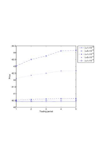
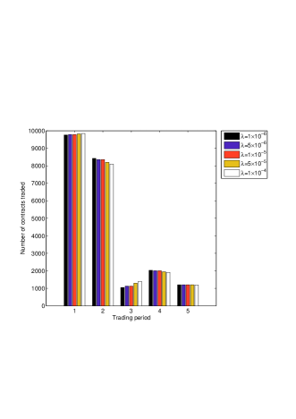
Figure 1: $\upsilon_{ij}=0$, $\epsilon_{ij}=0$ for all $i\in\left\{1,...,5\right\}$ and $j\in\left\{1\right\}$, and increasing $\lambda_{k}$ for all $k\in P\cup C$. The trading periods named by a number from 1 to 5 correspond to a two months ahead, a month ahead, a week ahead, a day ahead, and the spot price, respectively.

In Figure 2 we study the case when only the risk aversion of the producers is increased while the risk aversion of the consumers is kept constant. As we can see the risk aversion of the producers does not have any significant impact on the shape of the term structure of the price. However, the price of all contracts increased significantly due to the increased risk premium of the producers.

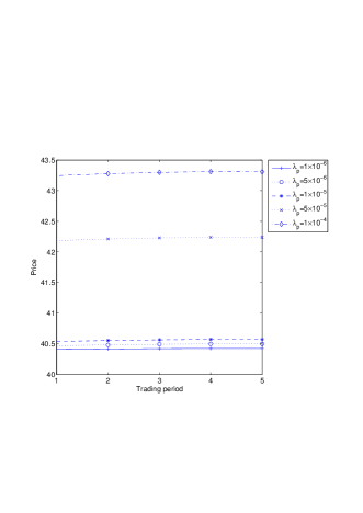
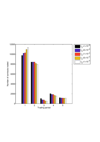
Figure 2: $\upsilon_{ij}=0$, $\epsilon_{ij}=0$ for all $i\in\left\{1,...,5\right\}$ and $j\in\left\{1\right\}$, $\lambda_{c}=10^{-6}$ for all $c\in C$, and increasing $\lambda_{p}$ for all $p\in P$.

In Figure 3 we study the case when only the risk aversion of the consumers is increased while the risk aversion of the producers is kept constant. We can see that this has a small impact on the term structure of the price. In contrast to the producers, the increased risk premium of the consumers is not reflected in an increased price. Thus, the consumers can only maintain their profitability by increasing the fixed price they charge the end users (i.e. they increase the constant price $s_{c}$ defined in (11)).

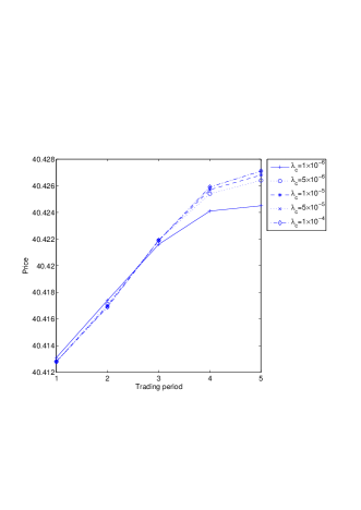
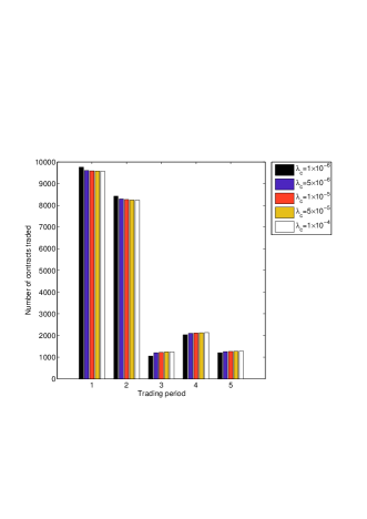
Figure 3: $\upsilon_{ij}=0$, $\epsilon_{ij}=0$ for all $i\in\left\{1,...,5\right\}$ and $j\in\left\{1\right\}$, $\lambda_{p}=10^{-6}$ for all $p\in P$, and increasing $\lambda_{c}$ for all $c\in C$.

One must increase the consumers’ risk aversion parameter $\lambda_{c}$ significantly to observe a visual impact. Such hypothetical case is depicted in Figure 4. We can see that by increasing the risk aversion of consumers, the term structure of electricity prices changes from the normal backwardation to contango. An increased risk aversion increases the consumers’ interest in less risky contracts and decreases the interest in risky contracts. Since the contracts closer to delivery are usually more risky, this causes the term structure to flip from normal backwardation to contango. A small kink at the fourth trading period is a consequence of a calibration of the covariance matrix on historical values.

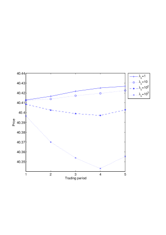
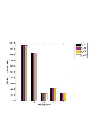
Figure 4: $\upsilon_{ij}=0$, $\epsilon_{ij}=0$ for all $i\in\left\{1,...,5\right\}$ and $j\in\left\{1\right\}$, $\lambda_{p}=10^{-6}$ for all $p\in P$, and increasing $\lambda_{c}$ for all $c\in C$.

Intuitively, it may not be immediately clear why the change in the risk aversion of producers and consumers has such a different impact on the term structure of the electricity price. The level of the price is defined by producers only. Let us consider a simplified setting when there is only one trading period and only one delivery period. Moreover, we have just one producer and one consumer. In such a setting, the profit of the consumer can be calculated as

(46) $$P_{c}\left(V_{c},\Pi\right)=e^{-\hat{r}T_{1}}\left(-\Pi\left(t_{1},T_{1}\right)+s_{c}\right)D\left(T_{1}\right)$$

where the constraint $V_{c}\left(t_{1},T_{1}\right)=D\left(T_{1}\right)$ was used. We can see that the profit function does not depend on the consumer’s decision variables $V_{c}$. Thus the consumer does not have any power to influence the price. She has to buy a sufficient amount of electricity to satisfy the demand of end users regardless of the electricity price. On the other hand, the producer has much more flexibility. Her profit can be calculated as

(47) $$P_{p}\left(V_{p},\Pi\right)=e^{-\hat{r}T_{1}}\left[-\Pi\left(t_{1},T_{1}\right)V_{p}\left(t_{1},T_{1}\right)-O_{p}\left(t_{1},T_{1}\right)G_{em}\left(t_{1},T_{1}\right)-\sum_{l\in L}G_{l}\left(t_{1},T_{1}\right)F_{p,l}\left(t_{1},T_{1}\right)\right].$$

An obvious feasible solution to her optimization problem (8) is

(48) $$V_{p}\left(t_{1},T_{1}\right)=O_{p}\left(t_{1},T_{1}\right)=F_{p,l}\left(t_{1},T_{1}\right)=0$$

for all $l\in L$. This leads to the objective value $\Phi_{p}=0$. Thus, clearly for any given price $\Pi\left(t_{1},T_{1}\right)$, the objective value satisfies $\Phi_{p}\geq 0$. A producer will only turn on the power plants if the electricity price is high enough to cover all production costs, trading costs, and the risk premium. A similar reasoning can also be extended to a multiperiod setting.

In Figures 5, 6, 7, and 8 we study the impact of the liquidity on the term structure of the electricity price. In Figures 5, and 6 the impact of the market micro-structure (i.e. the quadratic term $\upsilon$) is examined while in Figures 7, and 8 the impact of the bid-ask spread and the trading fees (i.e. the linear term $\epsilon$) is depicted.

Increasing of $\upsilon$ for all the contracts simultaneously (see Figure 5), increases the price without changing the shape of the term structure. It has a large impact on the optimal trading strategy of the players. When $\upsilon$ is large players spread the number of contracts traded in each trading period equally among all the trading periods available.

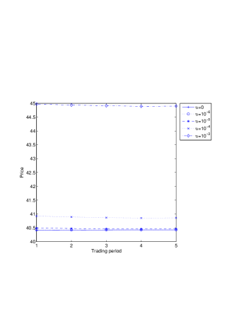
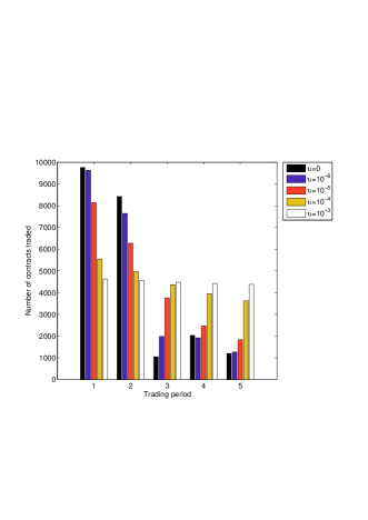
Figure 5: $\lambda_{k}=10^{-6}$ for all $k\in P\cup C$, $\epsilon_{ij}=0$ and increasing $\upsilon_{ij}$ for all $i\in\left\{1,...,5\right\}$ and $j\in\left\{1\right\}$.

When $\upsilon$ is changed only for the first trading period (i.e. the two month ahead contract), this significantly changes the term structure of the price. As we can see in Figure 6, a large increase in $\upsilon$ changes the term structure from normal backwardation to contango (i.e. downward sloping). As expected, the players also trade a much smaller number of contracts in the first trading period.

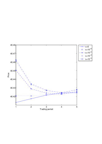
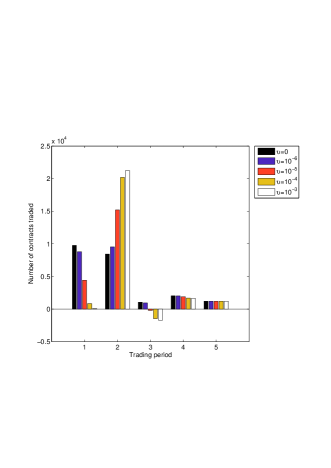
Figure 6: $\epsilon_{ij}=0$ for all $i\in\left\{1,...,5\right\}$ and $j\in\left\{1\right\}$, $\lambda_{k}=10^{-6}$ for all $k\in P\cup C$, and increasing $\upsilon_{11}$. For the other trading periods $i\in\left\{2,...,5\right\}$ and $j\in\left\{1\right\}$, $\upsilon_{ij}=0$.

An effect of a simultaneous change in the linear trading costs $\epsilon$ for all the contracts is depicted in Figure 7. We can see that the linear trading costs have no impact on the trading strategy and on the shape of the term structure. However, the price of all contracts is increased to cover the losses of the producers caused by the increased linear cost of trading. The consumers cover the losses caused by the increased linear cost of trading through increased electricity prices they charge to the end users. The simultaneous change in the linear trading costs $\epsilon$ for all the contracts does not impact the optimal trading strategy of the players.

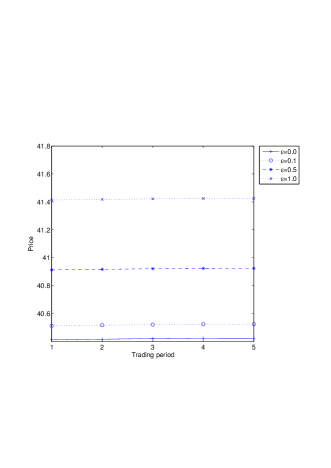
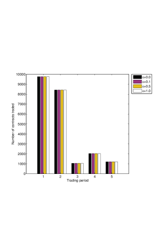
Figure 7: $\lambda_{k}=10^{-6}$ for all $k\in P\cup C$, $\upsilon_{ij}=0$ and increasing $\epsilon_{ij}$ for all $i\in\left\{1,...,5\right\}$ and $j\in\left\{1\right\}$.

When $\epsilon$ is changed only for the first trading period (i.e. the two month ahead contract), this, in contrast to the changes in $\upsilon$, significantly affects only the price in the first trading period. The price of the two month ahead contract is increased to cover the losses of the producers caused by the increased linear cost of trading. If $\epsilon$ is increased significantly, this makes the two month ahead contract so unattractive that no contracts are traded (see the right part of Figure 8).

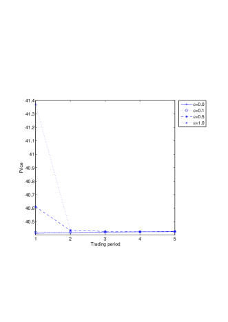
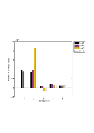
Figure 8: $\upsilon_{ij}=0$ for all $i\in\left\{1,...,5\right\}$ and $j\in\left\{1\right\}$, $\lambda_{k}=10^{-6}$ for all $k\in P\cup C$, and increasing $\epsilon_{11}$. For the other trading periods $i\in\left\{2,...,5\right\}$ and $j\in\left\{1\right\}$, $\epsilon_{ij}=0$.

In the reminder of this section, we investigate the effect of the term structure of fuel and emission prices on the term structure of electricity prices. Initially, we set

(49) $$\begin{array}[]{ccccccccc}\mathbb{E}^{\mathbb{P}}\left[G_{1}\left(t_{1},T_{1}\right)\right]&=&\mathbb{E}^{\mathbb{P}}\left[G_{1}\left(t_{2},T_{1}\right)\right]&=&\ldots&=&\mathbb{E}^{\mathbb{P}}\left[G_{1}\left(t_{5},T_{1}\right)\right]&=&69.30\>\left[\text{GBp/therm}\right],\\ \\ \mathbb{E}^{\mathbb{P}}\left[G_{2}\left(t_{1},T_{1}\right)\right]&=&\mathbb{E}^{\mathbb{P}}\left[G_{2}\left(t_{2},T_{1}\right)\right]&=&\ldots&=&\mathbb{E}^{\mathbb{P}}\left[G_{2}\left(t_{5},T_{1}\right)\right]&=&57.87\>\left[\text{GBP/tonne}\right],\\ \\ \mathbb{E}^{\mathbb{P}}\left[G_{em}\left(t_{1},T_{1}\right)\right]&=&\mathbb{E}^{\mathbb{P}}\left[G_{em}\left(t_{2},T_{1}\right)\right]&=&\ldots&=&\mathbb{E}^{\mathbb{P}}\left[G_{em}\left(t_{5},T_{1}\right)\right]&=&3.883\>\left[\text{GBP/tonne}\right],\end{array}$$

where $l=1$ and $l=2$ denote gas and coal prices, respectively. Electricity price is quoted in GBP/MWh.

We conducted two types of experiments: In the first type, we performed parallel shifts of the term structure of fuel/emission prices. In the second type, we changed the shape of the term structure of fuel/emission prices. Since results for all fuels as well as for emissions are very similar, we present them for gas only.

Figure 9 depicts the effect of parallel shifts in the term structure of gas prices. Expectedly, an increase/decrease in gas prices causes an increase/decrease in electricity prices.

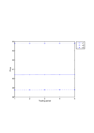
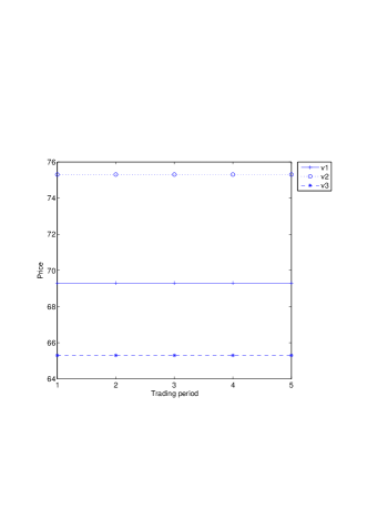
Figure 9: Effect of parallel shifts in the term structure of gas prices (right) on the term structure of electricity prices (left).

More interesting is the second experiment, where we calculated the term structure of electricity prices for three different shapes of the term structure of gas prices. In Figure 10, we examined a constant term structure of gas prices, normal backwardation and contango. We can see that the term structure of gas/emission prices has a large impact on the term structure of electricity prices.

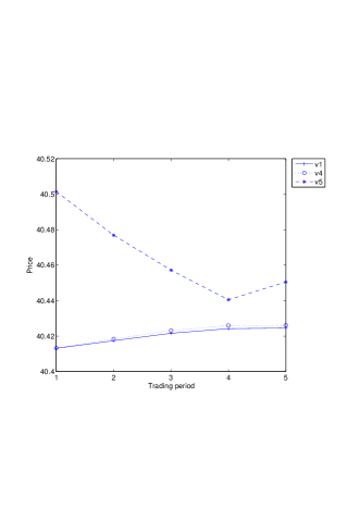
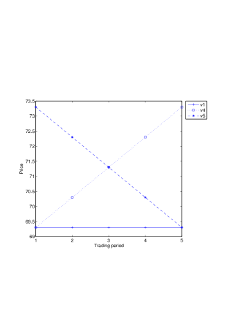
Figure 10: Dependence of the term structure of electricity prices (left) on the shape of the term structure of gas prices (right).

6.3 The UK power system

In this subsection we apply our model to the entire system of the UK power plants. We focus on the coal, gas, and oil power plants, because these power plants adapt their production to cover the changes in demand and are thus responsible for setting the price. Nuclear power plants do not have to be modeled explicitly because their ramp up and ramp down constraints are so tight that their production is almost constant over time. They usually deviate from the maximum production only for maintenance reasons. Renewable sources and interconnectors are not modeled explicitly, because they require a different treatment not covered in this paper. In this subsection, we define demand $D\left(T_{j}\right)$ for all $j\in J$ as

(50) $$D\left(T_{j}\right):=D_{act}\left(T_{j}\right)-P_{renw}\left(T_{j}\right)-P_{inter}\left(T_{j}\right)$$

where $D_{act}\left(T_{j}\right)$ denotes the actual demand in the UK power system, $P_{renw}\left(T_{j}\right)$ denotes the production from all renewable sources including wind, solar, biomass, hydro and pumped storage, and $P_{inter}\left(T_{j}\right)$ denotes the inflow of power in to the UK power system through interconnectors. To make this model useful in practice one has to model each of these terms, but this exceeds the scope of this paper.

We calibrate the model and for each power plant $r\in R^{p,l}$, $l\in L$ and $p\in P$, we estimate the efficiency $c^{p,l,r}$, the carbon emission intensity factor $g^{p,l,r}$, the maximum capacity $\overline{W}_{max}^{p,l,r}$, the ramp up rate $\triangle\overline{W}_{max}^{p,l,r}$ and the ramp down rate $\triangle\overline{W}_{min}^{p,l,r}$ using the historical production as described in Subsection 6.1. The covariance matrix was also estimated from the historical data using the shrinkage approach described in [17].

Our goal is to calculate the electricity spot price with the information available on 11/2/2013. We are interested in a delivery period from 4/4/2013 00:00:00 to 8/4/2013 00:00:00. We assume that there are two types of power contract available. The first is a month ahead contract traded on 15/3/2013 17:00:00 and covers the delivery over all four days. The second type is a spot contract that requires an immediate delivery and is traded for each half hour separately. We use future prices of coal, gas, and oil as available on 11/2/2013. Since the historical demand forecast is not available, we used the realized demand instead, which is a standard practice in the literature. To use this model in practice, one could use a demand forecast available at the Elexon web page or develop a new approach. Since we do not have the information about the ownership of the power plants, we assumed that there is only one producer who owns all power plants connected to the UK grid and only one consumer that is responsible for satisfying the demand of the end users. In reality, market participants have more information about the ownership that can be incorporated into the model.

The numerical results in Figures 11 - 14 are all calculated using $\lambda_{k}=10^{-5}$ for all $k\in P\cup C$, and $\epsilon_{ij}=0.1$ and $\upsilon_{ij}=10^{-4}$ for all contracts. The figure on the left hand side depicts the calculated energy mix between coal and gas power plants, while the figure on the right hand side depicts the actually observed energy mix. Both figures contain also the spot price calculated by our model and the actually observed spot price.

Figure 11 shows that our model predicts the energy mix very closely. Moreover, the daily pattern of the electricity price predicted by our model is similar to the actually observed one.

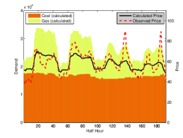
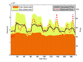
Figure 11: $\lambda_{k}=10^{-7}$ for all $k\in P\cup C$, $\epsilon=0.1$, and $\upsilon=10^{-4}$.

Figure 12 shows how the results change when we tighten the ramp up and ramp down constraints by 20%. We can see that the price is more serrated and slightly higher, because more expensive power plants must be turned on to cover the changes in demand.

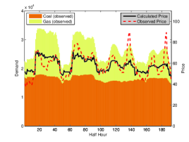
Figure 12: Ramp up and ramp down constraints are tightened by 20%.

Similarly, Figure 13 shows how the results change when we tighten the ramp up and ramp down constraints by 50%.

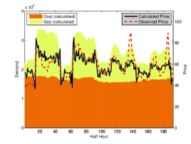
Figure 13: Ramp up and ramp down constraints are tightened by 50%.

Figure 11 reveals a few problems of our model. Firstly, we can see that the daily variation in the calculated price is smaller than in the observed one. Secondly, the two spikes in the observed price are not captured in our model. Our hypothesis is that the first problem occurs, because our model does not incorporate the start-up costs of the power plants correctly. Inclusion of the start-up costs exceeds the scope of this paper and will be addressed separately. Some preliminary results are shown in Figure 14. Our hypothesis for the explanation of the second problem is the error in the demand forecast. Spikes in the spot price occur when there is an unexpected change in demand. Since only a few (usually rather inefficient Open Cycle Gas Turbine) power plants are flexible enough to cover the demand, they require a high electricity price to be turned on. Thus, the spikes cannot be forecast two months before the delivery. An investigation of the predictive power of our model to forecast spikes closer to delivery is left for future work.

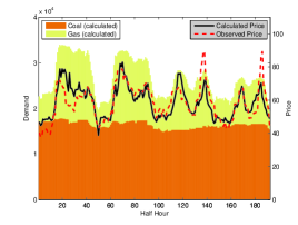
Figure 14: Preliminary result after including the startup costs.

7 Conclusions

In this paper we proposed a tractable quadratic programming reformulation for calculating the equilibrium term structure of electricity prices in a market with multiple consumers and producers. Reformulation can be used for solving general equilibrium optimization problems that include inequality constraints and can be seen as an extension of the shadow price approach.

We have extended the term structure electricity price model proposed in [21] to a more realistic setting by taking into account transaction costs and liquidity considerations as well as realistic electricity contracts.

The section on numerical results first shows how to calibrate various parameters of the model. We investigated how different parameters affect the equilibrium electricity price. Interestingly, we found that consumers have very little power to influence the electricity price. They have to satisfy the demand of the end users regardless of the price level. To maintain their profitability, they propagate all increased costs to the end users. Producers, on the other hand, have much more power to affect the electricity prices. They have a large impact on the price level and a slightly smaller impact on the term structure itself. The market micro-structure and liquidity of the contracts can significantly affect the term structure of the electricity price. In an extreme case, changes in the liquidity even altered the term structure from normal backwardation to contango. The term structure of electricity prices is also considerably affected by the term structure of fuels and emissions.

We investigated the predictive power of our model when applied to the realistic system of UK power plants. The results show that our model predicts the prices quite well and that the predicted price exhibits the main features of the electricity price. Numerical examples show the effect of tightened ramp up and ramp down constraints. We have also identified two areas where a further improvement is needed. Some very promising preliminary numerical results of the further improvements are also included.

References

• [1] R. Almgren and N. Chriss, Optimal execution of portfolio transactions, Journal of Risk, (2001), p. 5–39.
• [2] E. Anderson and H. Xu, Necessary and sufficient conditions for optimal offers in electricity markets, SIAM Journal on Control and Optimization, 41 (2002), pp. 1212–1228.
• [3]  , $\varepsilon$-optimal bidding in an electricity market with discontinuous market distribution function, SIAM Journal on Control and Optimization, 44 (2005), pp. 1391–1418.
• [4] M. T. Barlow, A diffusion model for electricity prices, Mathematical Finance, 12 (2002), pp. 287–298.
• [5] F. E. Benth and T. Meyer-Brandis, The information premium for non-storable commodities, Journal of Energy Markets, (2009).
• [6] H. Bessembinder and M. L. Lemmon, Equilibrium pricing and optimal hedging in electricity forward markets, Journal of Finance, 57 (2002), pp. 1347–1382.
• [7] W. Bühler, Risk premia of electricity futures: A dynamic equilibrium model, in Risk Management in Commodity Markets, John Wiley & Sons, Ltd., 2009, pp. 61–80.
• [8] W. Bühler and J. Müller-Merbach, Valuation of electricity futures: Reduced-form vs. dynamic equilibrium models, Mannheim Finance Working Paper No. 2007-07, (2009).
• [9] R. Carmona, M. Coulon, and D. Schwarz, Electricity price modeling and asset valuation: a multi-fuel structural approach, Mathematics and Financial Economics, 7 (2013), pp. 167–202.
• [10] L. Cavallo and V. Termini, Electricity derivatives and the spot market in italy. mitigating market power in the electricity market, (2005).
• [11] L. Clewlow and C. Strickland, A multi-factor model for energy derivatives, Research Paper Series 28, Quantitative Finance Research Centre, University of Technology, Sydney, Dec. 1999.
• [12]  , Valuing energy options in a one factor model fitted to forward prices, Research Paper Series 10, Quantitative Finance Research Centre, University of Technology, Sydney, Apr. 1999.
• [13] G. De Maere d’Aertrycke and Y. Smeers, Liquidity Risks on Power Exchanges: a Generalized Nash Equilibrium model, 2012.
• [14] I. Gurobi Optimization, Gurobi Optimizer Reference Manual, 2014.
• [15] B. Hambly, S. Howison, and T. Kluge, Modelling spikes and pricing swing options in electricity markets, Quantitative Finance, 9 (2009), p. 937–949.
• [16] S. Howison and M. C. Coulon, Stochastic behaviour of the electricity bid stack: From fundamental drivers to power prices, The Journal of Energy Markets, 2 (2009).
• [17] O. Ledoit and M. Wolf, Improved estimation of the covariance matrix of stock returns with an application to portfolio selection, Journal of Empirical Finance, 10 (2003), pp. 603–621.
• [18] J. J. Lucia and E. Schwartz, Electricity prices and power derivatives: Evidence from the nordic power exchange, (2000).
• [19] T. Meyer-Brandis and P. Tankov, Multi-factor jump-diffusion models of electricity prices, International Journal of Theoretical and Applied Finance (IJTAF), 11 (2008), pp. 503–528.
• [20] S. Robinson, Math model explains high prices in electricity markets, SIAM News, (2005).
• [21] M. Troha and R. Hauser, The existence and uniqueness of a power price equilibrium, ArXiv e-prints, (2014).