Quantum correlations and non-classicality in a system of two coupled vertical external cavity surface emitting lasers

Abstract

Here we demonstrate that photocurrent noise reduction below the standard quantum limit and modal anticorrelation can arise in two mode coupled two-VECSEL system with common pump. This effect occurs due to correlated loss of laser modes. It is possible to suppress noise below the standard quantum limit even for Poissonian coherent pumping, whereas the regularity of the pump can be harmful for non-classicality.

I Introduction

Semiconductor lasers are by far the commonest lasers that one finds around nowadays. However, despite being such a common device, they are still actively researched, modified and improved. They can be used for quantum communication/informatics, in particular, for generating non-classical states of radiation. Since the pioneering prediction by Golubev and Sokolov golubev1984 (and it was a quickly confirmed prediction teich1985 ), it is well known that a semiconductor laser driven by a regular low-noise current is able to produce photon-number squeezed states of light. One should have equal amounts of emitters of the active media pumped in equal intervals of time, so the emitted photons tend to be antibunched.

Here we demonstrate that the photocurrent noise suppression below the standard quantum limit (which is usually associated with photon-number squeezing) in semiconductor lasers (namely, in VECSEL lasers) can be reached by an entirely different mechanism. Namely, it can occur due to coupling of two modes to the same emitter with quickly decaying populations and polarization (which we shall term here as ”correlated loss”). And for this kind of noise reduction to appear, the regularity of the pump might be practically irrelevant.

It is well-known that coupling to the same emitter induces correlations between field reservoirs scully0 . Also, correlated losses are quite common in situations, where one has two or more systems (in our case, field modes) coupled to the third lossy system. Interference arising in this case was shown to lead to entanglement between modes even in absence of direct interaction between them entangle1 ; entangle2 . Correlated loss can lead to appearance of nonlinear coupling between modes and even to nonlinear loss producing nearly ideal Fock states mogilevtsev kerr 2009 ; mogilevtsev opt lett 2010 . Notice, that to have a correlated loss with all consequent nonlinear effects arising, one generally needs to have an hierarchy of time-scales present in the system. Dynamics of the modes should occur on much slower time-scale than dynamics of the dissipating systems coupled to these modes.

Here we demonstrate that in the system of two coupled vertical external cavity surface emitting lasers (VECSELs) with a common pump, a correlated loss can arise and lead to appearance of photocurrent noise reduction below the standard quantum limit (SQL). It occurs when this systems acts as a class-A laser, and the population inversion lifetime is much shorter, than the photon lifetimes in both modes. Since lasing emitters of the active media are coupled simultaneously to both modes, quick decaying emitters disentangle from them giving rise to effective non-linear coupling between modes (similarly to as dispersive atom-field produces Kerr nonlinearity in EIT media eit-kerr1 ; eit-kerr2 ; eit-kerr3 ). Excited emitters of the active media emit either in one or other mode without possibility to re-absorb emitted photon. Such an interference of emission channels gives rise to strong anti-correlation between modes. It was already demonstrated that VECSELs can be class-A lasers a-class1 ; a-class2 . Moreover, a scheme with coupled VECSELs generating two output linearly polarized modes of slightly different frequencies was recently realized in experiment and demonstrated as class-A laser pal2010 . This scheme we adopt as a basis for our theoretical model. We predict that in the set-up similar to the one used in Ref. pal2010 , noise reduction below SQL might occur for each individual mode. Also anticorrelation between modes can arise even for the Poissonian pumping (for example, with the active region excited by an external laser beam). However, our results are not limited to this particular scheme, and can be easily generalized to any kin of lasing devices with correlated loss.

The outline of the paper is as follows. In the second Section we introduce the model of two coupled VECSEL systems, write down quantum Langevin equations for them, discuss parameters of the scheme and describe how the correlated loss and nonlinearities can arise with the example of the simplified particular case of the scheme. In the third Section we derive equations for collective variables (polarizations and populations) and discuss a way to describe pump statistics taking into account partition noise. In Section IV we consider quasiclassical equations and demonstrate, that equations for modal amplitudes can be reduced to equations for A-class lasers. In Section V we investigate statistics of small fluctuations around stationary values of modal amplitudes, collective populations and polarizations, and discuss the obtained results.

II The model of two coupled VECSELS

Now let us consider a quantum model of two-frequency VECSEL in the configuration described in the paper pal2010 . There two coupled VECSELs were created by using two-modal external cavity with spatially separated modes. Spatial separation of modes was achieved by introducing a birefringent crystal inside the laser cavity. Modes overlap on the surface of the active media (which is rather thin for VECSEL lasers), and the pumped region encompasses all the surface. A schematic arrangement of the active media regions participating in the generation process can be seen in Fig.1(a).

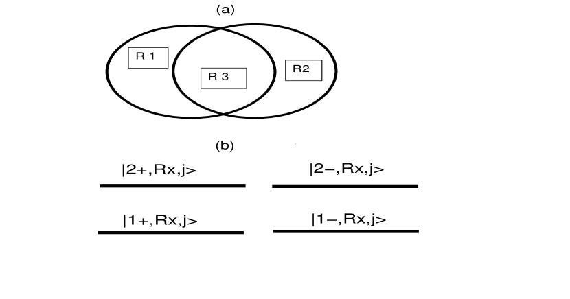
Figure 1: (a) An illustration of the active media regions generating lasing modes. Emitters of the region 1 (denoted as R1) interact only with modes denoted as ”a”, emitters of the region 2 (denoted as R2) interact only with modes denoted as ”b”; emitters of the region 3 (denoted as R3) interact with both groups of modes. (b) A scheme of levels of the $j$th emitter of region R$x$.

II.1 Basic equations

Considering our VECSEL model, we use already well established four-level spin-flip model for the description of emitters of the active media moloney1995 . For the single-frequency VECSEL the quantum theory was already extensively developed and elaborated on the basis of Langevin equation formalism kolobov2002 ; kolobov2004 . The model was shown to give quite accurate description of VECSELs’ lasing and to represent adequately a complicated polarization dynamics appearing in this kind of lasers. Each individual emitter/charge carrier of the active semiconductor in this model is described by a four-level system (actually, two two-level subsystems coupled by spin-flip interaction). Lower levels of this model correspond to the unexcited states of the semiconductor medium, i.e. without electron-hole pairs. Upper levels correspond to the excited states with electron-hole pairs. Two two-level subsystems are taken to represent states with different (and opposite) angular momenta. We assume that each two-level subsystem is coupled to the single circularly polarized mode with a direction of polarization corresponding to the angular momentum of the state, i.e. if one of the two-level subsystems is coupled to the right-polarized mode, than the other subsystem is coupled to the left-polarized one. The scheme of levels of the medium is depicted in Fig.1(b).

Now we proceed writing down a system of quantum Langevin equations for the interaction of the field with individual emitters along the lines indicated in Ref.kolobov2002 . Let us introduce bosonic annihilation operators, $\hat{a}_{\pm}$, $\hat{b}_{\pm}$ corresponding to circularly polarized (in opposite directions for $+$ and $-$) modes of groups ”a” and ”b”. Then, for these modal operators we have the following system of equations kolobov2002 :

$$\frac{d\hat{a}_{\pm}}{dt}=-(\kappa_{a}+i\omega_{a})\hat{a}_{\pm}-(\kappa_{ap}+i\omega_{ap})\hat{a}_{\mp}-$$

$$ig_{a}\Bigl{(}\sum\limits_{j\in R1}\Theta(t-t^{(1)}_{j})\sigma_{j\pm}^{-}+\sum\limits_{l\in R3}\Theta(t-t^{(3)}_{l})\sigma_{l\pm}^{-}\Bigr{)}+\hat{f}_{a\pm},$$

$$\frac{d\hat{b}_{\pm}}{dt}=-(\kappa_{b}+i\omega_{b})\hat{b}_{\pm}+(\kappa_{bp}+i\omega_{bp})\hat{b}_{\mp}-$$ (1)

$$ig_{b}\Bigl{(}\sum\limits_{k\in R2}\Theta(t-t^{(2)}_{k})\sigma_{k\pm}^{-}+\sum\limits_{l\in R3}\Theta(t-t^{(3)}_{l})\sigma_{l\pm}^{-}\Bigr{)}+\hat{f}_{b\pm},$$

where operators $\sigma_{j\pm}^{-}$ denote transition operators from the upper to lower level of the $j$th emitter for corresponding circular polarizations. Using notations of the state vectors corresponding to the emitter levels given in Fig.1, one writes

$$\sigma_{j\pm}^{-}=|1\pm,Rx,j\rangle\langle 2\pm,Rx,j|,\quad j\in Rx,$$

with $\sigma_{j\pm}^{+}$ being its Hermitian conjugate. Quantities $\kappa_{a,b}$ are decay rates for modes $a,b$. We assume that the linear dichroism is present, so, modes of different linear polarization decay with different rates. This difference is represented by parameters $\kappa_{ap}$ and $\kappa_{bp}$. Quantities $g_{a,b}$ are the emitter-field interaction constants for corresponding modes with frequencies $\omega_{a}$ and $\omega_{b}$, respectively. Parameters $\omega_{ap}$ and $\omega_{bp}$ represent coupling between modes of different circular polarization appearing due to linear birefringence.

For the model we adopt the simple injection-type pumping: an excited emitter (electron in the active zone and the hole in the valent zone) appears at a random time-moment. Step-functions $\Theta(t-t^{(x)}_{k})$ are describing such a process of driving the active media. So, the function $\Theta(t-t^{(x)}_{k})$ describes switching on the interaction of the field with the $k$th emitter of the $x$th region. Statistics of time moments, $t^{(x)}_{k}$, defines the type of the pumping (regular, Poissonian or else; for the details see Ref.scully ).

Operators $\hat{f}_{a,b\pm}$ represent quantum Langevin forces introduced into equations to account for quantum noises (in particular, to preserve correct commutation relation for modal operators). They are introduced in the standard manner (see, for example, a brilliant review by Luiz Davidovich davidovich ). We shall specify their properties later.

Now let us proceed with equations for single-emitter transition operators for different active regions depicted in Fig.1 :

$$\frac{d}{dt}\sigma_{j\pm}^{-}=-(\gamma_{\bot}+iw)\sigma_{j\pm}^{-}+\hat{f}_{j\pm}^{\sigma}+$$

$$ig_{a}\Theta(t-t^{(1)}_{j})(\hat{n}_{j\pm}^{(2)}-\hat{n}_{j\pm}^{(1)})\hat{a}_{\pm},\quad j\in R1,$$

$$\frac{d}{dt}\sigma_{j\pm}^{-}=-(\gamma_{\bot}+iw)\sigma_{j\pm}^{-}+\hat{f}_{j\pm}^{\sigma}+$$ (2)

$$ig_{b}\Theta(t-t^{(2)}_{j})(\hat{n}_{j\pm}^{(2)}-\hat{n}_{j\pm}^{(1)})\hat{b}_{\pm},\quad j\in R2$$

$$\frac{d}{dt}\sigma_{j\pm}^{-}=-(\gamma_{\bot}+iw)\sigma_{j\pm}^{-}+\hat{f}_{j\pm}^{\sigma}+$$

$$i\Theta(t-t^{(3)}_{j})(\hat{n}_{j\pm}^{(2)}-\hat{n}_{j\pm}^{(1)})(g_{a}\hat{a}_{\pm}+g_{b}\hat{b}_{\pm}),\quad j\in R3.$$

Here the parameter $\gamma_{\bot}$ is the dephasing rate of two-level subsystems of the emitter; $w$ is the transition frequency. Operators $\hat{n}_{j\pm}^{(y)}$ describe population of $y$th level of $j$th emitter of the $x$th region:

$$\hat{n}_{j\pm}^{(2)}=|2\pm,Rx,j\rangle\langle 2\pm,Rx,j|,$$

$$\hat{n}_{j\pm}^{(1)}=|1\pm,Rx,j\rangle\langle 1\pm,Rx,j|,$$

where $j\in Rx$. Operators $\hat{f}_{j\pm}^{\sigma}$ represent the corresponding Langevin forces; these operators are independent. We discuss them in the next Subsection.

Finally, let us write down equations for single-emitter operators describing populations. For upper levels these are

$$\frac{d}{dt}\hat{n}_{j\pm}^{(2)}=-\gamma_{2}\hat{n}_{j\pm}^{(2)}-\gamma_{c}(\hat{n}_{j\pm}^{(2)}-\hat{n}_{j\mp}^{(2)})+$$

$$ig_{a}\Theta(t-t^{(1)}_{j})(\hat{a}^{\dagger}_{\pm})\sigma_{j\pm}^{-}-\mathrm{h.c.})+\hat{f}_{j\pm}^{(2)},\quad j\in R1,$$

$$\frac{d}{dt}\hat{n}_{j\pm}^{(2)}=-\gamma_{2}\hat{n}_{j\pm}^{(2)}-\gamma_{c}(\hat{n}_{j\pm}^{(2)}-\hat{n}_{j\mp}^{(2)})+$$ (3)

$$ig_{b}\Theta(t-t^{(2)}_{j})(\hat{b}^{\dagger}_{\pm})\sigma_{j\pm}^{-}-\mathrm{h.c.})+\hat{f}_{j\pm}^{(2)},\quad j\in R2,$$

$$\frac{d}{dt}\hat{n}_{j\pm}^{(2)}=-\gamma_{2}\hat{n}_{j\pm}^{(2)}-\gamma_{c}(\hat{n}_{j\pm}^{(2)}-\hat{n}_{j\mp}^{(2)})+$$

$$+i\Theta(t-t^{(3)}_{j})((g_{a}\hat{a}^{\dagger}_{\pm}+g_{b}\hat{b}^{\dagger}_{\pm})\sigma_{j\pm}^{-}-\mathrm{h.c.})+\hat{f}_{j\pm}^{(2)},\quad j\in R3.$$

Here $\gamma_{2}$ is the decay rate of the emitter’s upper levels; $\gamma_{c}$ is the rate of spin-flips between levels $|2+,Rx,j\rangle$ and $|2-,Rx,j\rangle$. Operators $\hat{f}_{j\pm}^{(2)}$ represent corresponding Langevin forces.

Equations for populations of lower levels are as follows:

$$\frac{d}{dt}\hat{n}_{j\pm}^{(1)}=-\gamma_{1}\hat{n}_{j\pm}^{(1)}+\hat{f}_{j\pm}^{(1)}-$$

$$ig\Theta(t-t^{(1)}_{j})(\hat{a}^{\dagger}_{\pm}\sigma_{j\pm}^{-}-\mathrm{h.c.}),\quad j\in R1,$$

$$\frac{d}{dt}\hat{n}_{j\pm}^{(1)}=-\gamma_{1}\hat{n}_{j\pm}^{(1)}+\hat{f}_{j\pm}^{(1)}-$$ (4)

$$ig\Theta(t-t^{(2)}_{j})(\hat{b}^{\dagger}_{\pm}\sigma_{j\pm}^{-}-\mathrm{h.c.}),\quad j\in R2,$$

$$\frac{d}{dt}\hat{n}_{j\pm}^{(1)}=-\gamma_{1}\hat{n}_{j\pm}^{(1)}-+\hat{f}_{j\pm}^{(1)}-$$

$$ig\Theta(t-t^{(3)}_{j})((\hat{a}^{\dagger}_{\pm}+\hat{b}^{\dagger}_{\pm})\sigma_{j\pm}^{-}-\mathrm{h.c.}),\quad j\in R3.$$

Here $\gamma_{1}$ is the decay rate of the emitter’s lower levels; operators $\hat{f}_{j\pm}^{(1)}$ represent corresponding Langevin forces. Notice, that we are assuming no spin-flips between lower levels of emitters. It is really unimportant for the considered scheme because the decay rate of lower levels, $\gamma_{1}$, is taken to be far exceeding that of upper levels, $\gamma_{2}$.

II.2 Langevin forces

Here we describe Langevin forces in Eqs. (II.1,II.1,II.1,II.1). First of all, they are $\delta$-correlated, i.e. for any two forces $\hat{f}_{x}(t)$ and $\hat{f}_{y}(\tau)$ one has

$$\langle\hat{f}_{x}(t)\hat{f}_{y}(\tau)\rangle=d_{xy}(t)\delta(t-\tau),$$

where brackets $\langle\ldots\rangle$ denote quantum averaging. So, $d_{xt}(t)$ are c-number functions. However, they do generally depend on stochastic variables, namely, emitter arrival times. First-order averages of Langevine forces are zero: $\langle\hat{f}_{x}(t)\rangle=0$.

Then, we assume that Langevin forces for different emitters of different regions are independent quantum variables, so, for any two forces corresponding to variables of different emitters, $\hat{f}_{Rj}(t)$ and $\hat{f}_{Rk}(\tau)$, $j\neq k$, one has $\langle\hat{f}_{Rj}(t)\hat{f}_{Rk}(\tau)\rangle=0$. Equally, quantum Langevin forces for modes of $a$ and $b$ groups are independent.

Thus, we proceed to non-zero second-order correlation functions along the lines given in Refs.kolobov2002 ; davidovich . Assuming that there is practically no thermal noise of field modes at optical frequencies, one has

$$\langle\hat{f}_{x\pm}(t)\hat{f}_{x\pm}^{\dagger}(\tau)\rangle=2\kappa_{x}\delta(t-\tau),$$

$$\langle\hat{f}_{x\pm}(t)\hat{f}_{x\mp}^{\dagger}(\tau)\rangle=2\kappa_{xp}\delta(t-\tau),$$ (5)

where $x=a,b$.

The operators of Langevin forces for emitters’ populations are self-conjugated, so in all regions one has

$$\langle\hat{f}_{j\pm}^{(2)}(t)\hat{f}_{j\pm}^{(2)}(\tau)\rangle=\delta(t-\tau)\times$$

$$\left[\gamma_{2}\langle\hat{n}_{j\pm)}^{(2)}\rangle+\gamma_{c}(\langle\hat{n}_{j\pm}^{(2)}\rangle+\langle\hat{n}_{j\mp}^{(2)}\rangle)\right],$$

$$\langle\hat{f}_{j\pm}^{(2)}(t)\hat{f}_{j\mp}^{(2)}(\tau)\rangle=-\delta(t-\tau)\times$$ (6)

$$\gamma_{c}(\langle\hat{n}_{j\pm}^{(2)}\rangle+\langle\hat{n}_{j\mp}^{(2)}\rangle),$$

$$\langle\hat{f}_{j\pm}^{(1)}(t)\hat{f}_{j\pm}^{(1)}(\tau)\rangle=\gamma_{1}\langle\hat{n}_{j\pm}^{(1)}\rangle\delta(t-\tau).$$

For transition operators one has in the same way

$$\Bigl{\langle}\left[\hat{f}_{j\pm}^{\sigma}(t)\right]^{\dagger}\hat{f}_{j\pm}^{\sigma}(\tau)\Bigr{\rangle}=\delta(t-\tau)\times$$

$$\left[(2\gamma_{\bot}-\gamma_{2}-\gamma_{c})\langle\hat{n}_{j\pm}^{(2)}\rangle+\gamma_{c}\langle\hat{n}_{j\mp}^{(2)}\rangle\right],$$

$$\Bigl{\langle}\hat{f}_{j\pm}^{\sigma}(t)\left[\hat{f}_{j\pm}^{\sigma}(\tau)\right]^{\dagger}\Bigr{\rangle}=\delta(t-\tau)\times$$ (7)

$$(2\gamma_{\bot}-\gamma_{1})\langle\hat{n}_{j\pm}^{(1)}\rangle.$$

Finally, we write down cross-correlations of Langevin forces for transition operators and populations:

$$\langle\hat{f}_{j\pm}^{\sigma}(t)\hat{f}_{j\pm}^{(2)}(\tau)\rangle=(\gamma_{2}+\gamma_{c})\langle\sigma_{j\pm}\rangle\delta(t-\tau)$$

$$\langle\hat{f}_{j\pm}^{\sigma}(t)\hat{f}_{j\mp}^{(2)}(\tau)\rangle=-\gamma_{c}\langle\sigma_{j\pm}\rangle\delta(t-\tau),$$ (8)

$$\Bigl{\langle}\left[\hat{f}_{j\pm}^{\sigma}(t)\right]^{\dagger}\hat{f}_{j\pm}^{(1)}(\tau)\Bigr{\rangle}=\gamma_{1}\langle\sigma_{j\pm}^{\dagger}\rangle\delta(t-\tau),$$

also valid for all three regions.

II.3 Parameters of the scheme

We consider realistic values of parameters of the scheme outlined above in this Section. They are close to those of the experiment described in Ref. pal2010 . For these values the scheme acts as a class-A laser. First of all, we assume that the lower levels of emitters are emptied very rapidly, i.e. $\gamma_{1}$ is sufficiently large to exclude adiabatically the lower level populations. Actually, rapid decay of lower level populations is a condition of this model applicability for semiconductor lasers; see, for example, Ref.jacobino1997 . Then, we make a realistic assumption about dephasing in the active media being very rapid, so the decay rate, $\gamma_{\bot}$, far exceeds the upper levels decay rate, $\gamma_{2}$. Finally, we make an assumption of the class-A laser: we take upper level decay rate to be far exceeding modal decay rates, $\kappa_{a,b}$ and $\kappa_{ap,bp}$. So, the following hierarchy for the time-scales takes place in our model:

$$\kappa_{a,b},\kappa_{ap,bp}\ll\gamma_{2}\ll\gamma_{\bot},\gamma_{1}.$$ (9)

Also, we assume that the interaction constants $g_{a,b}$ are small in comparison with the the upper levels decay rate, $\gamma_{2}$.

II.4 Toy model for correlated loss

Now let us demonstrate that satisfying the condition (9), one can get a nonlinear coupling between modes. For illustration we take the simplified model of just two field modes of the same frequency coupled resonantly to a single two-level system subjected to strong dephasing and population loss. We describe this simplified model with the following master equation for the density matrix, $\rho$, written in the basis rotated with the emitters transition frequency

$${d\over dt}\rho=-ig[\sigma^{+}(a+b)+h.c.,\rho]+$$

$$(\gamma_{\bot}\mathcal{L}(\sigma_{z})+\gamma_{2}\mathcal{L}(\sigma^{-}))\rho,$$ (10)

where the dissipator $\mathcal{L}(x)\rho=2x\rho x^{\dagger}-x^{\dagger}x\rho-\rho x^{\dagger}x$.

The condition (9) allows one to eliminate adiabatically off-diagonal matrix elements $\langle k|\rho|l\rangle$; where $k,l=1,2;\quad k\neq l$, since they decay with a large rate dephasing rate, $\gamma_{\bot}$. For times much exceeding $\gamma_{\bot}^{-1}$ one can write

$$\langle k|\rho|l\rangle\approx-i\frac{g^{2}}{\gamma_{\bot}}\langle k|\hat{n}\sigma_{z}\rho|l\rangle,$$

where $\hat{n}=(a^{\dagger}+b^{\dagger})(a+b)$.

So, the master equation is reduced to one describing a dispersive coupling of modes with a two-level system:

$${d\over dt}\rho\approx-2i\frac{g^{2}}{\gamma_{\bot}}[\hat{n}\sigma_{z},\rho]+\gamma_{2}\mathcal{L}(\sigma^{-})\rho$$ (11)

Obviously, a coupling between modes has arisen as a consequence of correlated loss. So, modes become correlated even in the absence of direct coupling between them as the result of strong decay of the emitters coupled to the modes.

Moreover, under conditions leading to the dispersive coupling similar to Eq.(11), Kerr nonlinearities can arise, too eit-kerr1 ; eit-kerr2 ; eit-kerr3 . Indeed, adiabatically eliminating emitter variables from Eq. (10) while retaining terms up to $g^{3}/\gamma_{\bot}^{3}$ and averaging over the state of emitter, it is not hard to obtain for the reduced density matrix the following expression

$${d\over dt}\hat{\rho}\approx-2i\frac{g^{2}}{\gamma_{\bot}}[\hat{n},\hat{\rho}]-4i\frac{g^{4}}{\gamma_{\bot}^{3}}[\hat{n}^{2},\hat{\rho}].$$ (12)

Thus, one has both linear and cross-Kerr coupling between the modes. Provided that modal losses are sufficiently low, self-Kerr and cross-Kerr nonlinearities appearing in Eq.(12) are known to be able to lead both to photon number squeezing of individual modes and to anticorrelations of modes eit-kerr1 ; eit-kerr2 ; eit-kerr3 ; kerr_all . As it will be seen below, it is just the case for our class-A coupled VECSELs lasers.

III Collective equations

The next step is to move from single-emitter equations to equations for collective operators describing ensembles of emitters in different regions of active media. Such collective operators can be introduced in a standard manner (see, for example, Refs.kolobov2002 ; scully ; davidovich ). So, introducing for clarity different notations for different regions, we obtain for polarizations

$$\hat{P}_{\pm}=-i\sum\limits_{j\in R1}\Theta(t-t^{(1)}_{j})\sigma_{j\pm}^{-},$$

$$\hat{Q}_{\pm}=-i\sum\limits_{j\in R2}\Theta(t-t^{(2)}_{j})\sigma_{j\pm}^{-},$$ (13)

$$\hat{\Xi}_{\pm}=-i\sum\limits_{j\in R3}\Theta(t-t^{(3)}_{j})\sigma_{j\pm}^{-}.$$

For collective population operators we have

$$\hat{M}_{y\pm}=\sum\limits_{j\in R1}\Theta(t-t^{(1)}_{j})\hat{n}_{j\pm}^{(y)},$$

$$\hat{N}_{y\pm}=\sum\limits_{j\in R2}\Theta(t-t^{(2)}_{j})\hat{n}_{j\pm}^{(y)},$$ (14)

$$\hat{\Lambda}_{y\pm}=\sum\limits_{j\in R3}\Theta(t-t^{(3)}_{j})\hat{n}_{j\pm}^{(y)}.$$

where $y=1,2$ denotes the emitter level.

In this section we derive equations for collective variables (III,III), perform averaging over arrival times of emitters via injection-like pumping and calculate quantum Langevin forces corresponding to the introduced collective operators.

III.1 Equations for collective variables

First of all, let us write equations for modal operators. From the system (II.1) one has

$$\frac{d\hat{a}_{\pm}}{dt}=-(\kappa_{a}+i\omega_{a})\hat{a}_{\pm}+(\kappa_{ap}+i\omega_{ap})\hat{a}_{\mp}+$$

$$g_{a}(\hat{P}_{\pm}+\hat{\Xi}_{\pm})+\hat{f}_{a\pm},$$

$$\frac{d\hat{b}_{\pm}}{dt}=-(\kappa_{b}+i\omega_{b})\hat{b}_{\pm}+(\kappa_{bp}+i\omega_{bp})\hat{b}_{\mp}+$$ (15)

$$g_{b}(\hat{Q}_{\pm}+\hat{\Xi}_{\pm})+\hat{f}_{b\pm},$$

As follows from Eqs.(II.1,III,III), equations for collective polarization operators are

$$\frac{d}{dt}\hat{P}_{\pm}=-(\gamma_{\bot}+iw)\hat{P}_{\pm}+$$

$$g_{a}(\hat{M}_{2\pm}-\hat{M}_{1\pm})\hat{a}_{\pm}+\hat{F}_{\pm}^{P},$$

$$\frac{d}{dt}\hat{Q}_{\pm}=-(\gamma_{\bot}+iw)\hat{Q}_{\pm}+$$ (16)

$$g_{b}(\hat{N}_{2\pm}-\hat{N}_{1\pm})\hat{b}_{\pm}+\hat{F}_{\pm}^{Q},$$

$$\frac{d}{dt}\hat{\Xi}_{\pm}=-(\gamma_{\bot}+iw)\hat{\Xi}_{\pm}+$$

$$(\hat{\Lambda}_{2\pm}-\hat{\Lambda}_{1\pm})(g_{a}\hat{a}_{\pm}+g_{b}\hat{b}_{\pm})+\hat{F}_{\pm}^{\Xi}.$$

Collective Langevin operators for these equations are

$$\hat{F}_{\pm}^{P,Q,\Xi}=\sum\limits_{j\in R1,R2,R3}\delta(t-t^{(1,2,3)}_{j})\sigma_{j\pm}^{-}+$$

$$\sum\limits_{j\in R1,R2,R3}\Theta(t-t^{(1,2,3)}_{j})\hat{f}_{j\pm}^{\sigma}.$$ (17)

Correlation properties for these operators will be given in the next Subsection.

Equations for collective populations are not so trivial to derive as those given above. Eqs. (III.1,III.1) remain invariant after averaging over arrival times (of course, it holds, if one assumes that operators in these equations are not correlated through it; such an assumption is obviously valid near the stationary regime that we are mostly interested in; see Ref.scully ). It is not so for equations describing collective populations, since the noise for populations is biased (has non-zero average) due to presence of the pump. We assume that emitters arrive fully excited, and become with equal probability either $+$ or $-$ excited subsystem of each VECSEL. Let us for the time being denote these biases for the upper-level population collective noises as $R_{x}$, $x$, denoting regions as in Fig.1. As follows from Eqs.(II.1,III,III), equations for operators of total upper-state populations are

$$\frac{d}{dt}\hat{M}_{2\pm}=R_{1}-\gamma_{2}\hat{M}_{2\pm}-\gamma_{c}(\hat{M}_{2\pm}-\hat{M}_{2\mp})-$$

$$g_{a}(\hat{a}_{\pm}^{\dagger}\hat{P}_{\pm}+\hat{P}^{\dagger}_{\pm}\hat{a}_{\pm})+\hat{F}_{2\pm}^{M},$$

$$\frac{d}{dt}\hat{N}_{2\pm}=R_{2}-\gamma_{2}\hat{N}_{2\pm}-\gamma_{c}(\hat{N}_{2\pm}-\hat{N}_{2\mp})-$$ (18)

$$g_{b}(\hat{b}_{\pm}^{\dagger}\hat{Q}_{\pm}+\hat{Q}^{\dagger}_{\pm}\hat{b}_{\pm})+\hat{F}_{2\pm}^{N},$$

$$\frac{d}{dt}\hat{\Lambda}_{2\pm}=R_{3}-\gamma_{2}\hat{\Lambda}_{2\pm}-\gamma_{c}(\hat{\Lambda}_{2\pm}-\hat{\Lambda}_{2\mp})-$$

$$((g_{a}\hat{a}_{\pm}^{\dagger}+g_{b}\hat{b}_{\pm}^{\dagger})\hat{\Xi}_{\pm}+\hat{\Xi}^{\dagger}_{\pm}(g_{a}\hat{a}_{\pm}+g_{b}\hat{b}_{\pm}))+\hat{F}_{2\pm}^{\Lambda}.$$

In the system (III.1) the collective Langevin operators are

$$\hat{F}_{2\pm}^{M,N,\Lambda}=\sum\limits_{j\in R1,R2,R3}\delta(t-t^{(1,2,3)}_{j})\hat{n}^{(2)}_{j\pm}+$$

$$\sum\limits_{j\in R1,R2,R3}\Theta(t-t^{(1,2,3)}_{j})\hat{f}_{j\pm}^{(2)}-R_{1,2,3}.$$ (19)

From the equation (19) it is clear that parameters $R_{1,2,3}$ are average pump rates (i.e. emitter injection rates) of emitters of the certain type (i.e. $+$ or $-$) in corresponding regions. Indeed, it is easy to see that with our way of driving one has (see the derivation in Ref. kolobov2002 )

$$\left\langle\sum\limits_{j\in R1,R2,R3}\delta(t-t^{(1,2,3)}_{j})\hat{n}_{j\pm}^{(2)}\right\rangle_{s}=R_{1,2,3},$$

where $\langle\ldots\rangle_{s}$ denoted averaging over the arrival times.

In our scheme of two-frequency VECSEL the pumping source for all three regions is the same pal2010 . So, respective pump rates are not independent parameters. Since we are assuming that density of emitters is the same in all considered regions, the average pump rate for every region is simply proportional to the size of this region. Thus, we write

$$R_{3}=\sqrt{\xi_{a}}(R_{1}+R_{3})=\sqrt{\xi_{b}}(R_{2}+R_{3})$$ (20)

where parameters $\xi_{a,b}$ describe the respective sizes of the regions of modal overlap, $R_{3}$, relative to total sizes of regions interacting with modes ”a” and ”b”.

Finally, we write down equations for lower level collective populations deriving them from Eqs.(II.1). Notice that emitters are taken to be injected being completely excited, i.e. they are on upper levels. Thus, we have

$$\frac{d}{dt}\hat{M}_{1\pm}=-\gamma_{1}\hat{M}_{1\pm}+\hat{F}_{1\pm}^{M}+$$

$$g_{a}(\hat{a}_{\pm}^{\dagger}\hat{P}_{\pm}+\hat{P}^{\dagger}_{\pm}\hat{a}_{\pm}),$$

$$\frac{d}{dt}\hat{N}_{1\pm}=-\gamma_{1}\hat{N}_{1\pm}+\hat{F}_{1\pm}^{N}+$$ (21)

$$g_{b}(\hat{b}_{\pm}^{\dagger}\hat{Q}_{\pm}+\hat{Q}^{\dagger}_{\pm}\hat{b}_{\pm}),$$

$$\frac{d}{dt}\hat{\Lambda}_{\pm}=-\gamma_{2}\hat{\Lambda}_{\pm}+\hat{F}_{1\pm}^{\Lambda}+$$

$$((g_{a}\hat{a}_{\pm}^{\dagger}+g_{b}\hat{b}_{\pm}^{\dagger})\hat{\Xi}_{\pm}+\hat{\Xi}^{\dagger}_{\pm}(g_{a}\hat{a}_{\pm}+g_{b}\hat{b}_{\pm})).$$

In this system the collective Langevin operators are

$$\hat{F}_{1\pm}^{M,N,\Lambda}=\sum\limits_{j\in R1,R2,R3}\delta(t-t^{(1,2,3)}_{j})\hat{n}_{j\pm}^{(1)}+$$

$$\sum\limits_{j\in R1,R2,R3}\Theta(t-t^{(1,2,3)}_{j})\hat{f}_{j\pm}^{(1)}.$$ (22)

It should be pointed out that statistics of arriving times, $t_{j}^{1,2,3}$ is defined by the character of the driving process and might influence states of the emitted modes. This statistics affects correlation properties of Langevin operators, which are to be discussed in the next Subsection.

III.2 Correlations functions for collective Langevin operators

Notwithstanding the fact that collective variables are composed only from emitter operators of the same region, operators of collective Langevin forces for different regions are not independent and their cross-correlations are not always zero. It occurs because of the presence of the same driving source for all three regions. Naturally, such a driving partition can give rise to cross-region correlations. Here we consider them generalizing a simple and illustrative procedure described in details in Ref.scully . Using it, one obtains that

$$\left\langle\sum\limits_{j\in Rx,k\in Ry}\delta(t-t^{(x)}_{j})\delta(t-t^{(y)}_{k})\hat{n}_{j\pm}^{(2)}\hat{n}_{k\pm}^{(2)}\right\rangle_{s}=$$

$$(R_{x}+R_{x}^{2})\delta_{xy}-\frac{R_{x}R_{y}}{R}\frac{p}{2},$$ (23)

where the parameter $p$ describes the regularity of the pump and $R=R_{1}+R_{2}+R_{3}$. The value $p=0$ corresponds to the Poissonian pump (for example, as it is for pumping the active region with the external laser field in Ref.pal2010 ). The value $p=1$ corresponds to the regular pump when emitters arrive to the active region with a constant rate. However, even in this case either ”+” or ”-” subsystems are excited with equal probability; that is the reason of having $p/2$ instead of $p$ in Eq.(23). Values $0<p<1$ correspond to partially regular pumping. One can see from Eq.(23) that for Poissonian pump noise correlations between region do not arise, whereas for regular pumping one has cross-region correlations. As we shall see below, such a partition noise negates a noise-suppression effect of the regular pump. Photon number squeezing in our two coupled VECSELs scheme arise solely due to effect of the correlated loss, i.e. due to interference of emission channels.

Thus, from Eqs.(19) it is possible to get second-order correlation functions of the collective Langevin forces for collective upper-state populations. For non-zero correlation functions of the same regions one has

$$\left\langle\hat{F}_{2\pm}^{Y}(t)\hat{F}_{2\pm}^{Y}(\tau)\right\rangle=\delta(t-\tau)R_{y}\left(1-\frac{R_{y}}{R}\frac{p}{2}\right)+$$

$$\delta(t-\tau)\left(\gamma_{2}Y_{2\pm}+\gamma_{c}(Y_{2\pm}+Y_{2\mp})\right),$$

$$\left\langle\hat{F}_{2\pm}^{Y}(t)\hat{F}_{2\mp}^{Y}(\tau)\right\rangle=-\delta(t-\tau)\frac{R_{y}^{2}}{R}\frac{p}{2}-$$ (24)

$$\gamma_{c}\delta(t-\tau)\left(Y_{2\pm}+Y_{2\mp}\right),$$

where $Y=M,N,\Lambda$, and, simultaneously, $y=1,2,3$. For cross-correlation functions of different regions one has

$$\left\langle\hat{F}_{2\pm}^{X}(t)\hat{F}_{2\pm}^{Y}(\tau)\right\rangle=\left\langle\hat{F}_{2\pm}^{X}(t)\hat{F}_{2\mp}^{Y}(\tau)\right\rangle=$$

$$-\delta(t-\tau)\left(\frac{R_{x}R_{y}}{R}\frac{p}{2}\right),\quad X\neq Y,\quad x\neq y,$$ (25)

where $X,Y=M,N,\Lambda$, and, simultaneously, $x,y=1,2,3$. Variables without ”hats” denote averages of corresponding quantum variables, i.e. $\langle\hat{s}\rangle=s$, and averaging is assumed to be done over the distribution of arrival times, too.

Since the emitters arrive completely excited, non-zero second-order correlation functions of the collective Langevin forces for collective lower-state populations are simpler than Eqs. (III.2,25):

$$\left\langle\hat{F}_{1\pm}^{Y}(t)\hat{F}_{1\pm}^{Y}(\tau)\right\rangle=\delta(t-\tau)\gamma_{1}{Y}_{1\pm},$$ (26)

where $Y=M,N,\Lambda$.

For auto-correlation functions of collective polarizations one has

$$\left\langle\left[\hat{F}_{\pm}^{Y}(t)\right]^{\dagger}\hat{F}_{\pm}^{Y}(\tau)\right\rangle=\delta(t-\tau)\times$$

$$\left((2\gamma_{\bot}-\gamma_{2}-\gamma_{c}){Y}_{2\pm}+\gamma_{c}{Y}_{2\mp}+R_{y}\right),$$ (27)

$$\left\langle\hat{F}_{\pm}^{Y}(t)\left[\hat{F}_{\pm}^{Y}(\tau)\right]^{\dagger}\right\rangle=\delta(t-\tau)(2\gamma_{\bot}-\gamma_{1}){Y}_{1\pm},$$

where $Y=M,N,\Lambda$ and, simultaneously, $y=1,2,3$.

For non-zero cross-correlation functions of noises of collective polarization and populations for the same region it follows from Eqs.(17,19,22) that

$$\left\langle\hat{F}_{\pm}^{X}(t)\hat{F}_{2\pm}^{Y}(\tau)\right\rangle=\delta(t-\tau)(\gamma_{2}+\gamma_{c}){X}_{\pm},$$

$$\left\langle\hat{F}_{\pm}^{X}(t)\hat{F}_{2\mp}^{Y}(\tau)\right\rangle=-\delta(t-\tau)\gamma_{c}{X}_{\pm},$$ (28)

$$\left\langle\left[\hat{F}_{\pm}^{X}(t)\right]^{\dagger}\hat{F}_{2\mp}^{Y}(\tau)\right\rangle=\delta(t-\tau)\gamma_{1}{X}_{\pm}^{\ast}.$$

where $X=P,Q,\Xi$ and, simultaneously, $Y=M,N,\Lambda$.

Correlation functions derived in this Subsection will be used for analyzing small fluctuations around stationary solutions of Eqs. (III.1,III.1,III.1,III.1).

IV Quasiclassical equations and stationary solutions

In this Section we analyze collective equations (III.1,III.1,III.1,III.1) in the quasiclassical limit, when one neglects quantum correlations between variables, i.e. assumes that for any two variables $\langle xy\rangle\approx\langle x\rangle\langle y\rangle$. We shall consider the case where only two linearly and orthogonally polarized modes persist in the whole system in the stationary regime. Thus, we assume that for sufficiently large evolution times, $t\rightarrow\infty$, only amplitudes

$$a_{x}=\frac{1}{\sqrt{2}}(a_{+}+a_{-})$$

and

$$b_{y}=\frac{i}{\sqrt{2}}(b_{-}-b_{+})$$

are non-zero. This regime was realized in the experiment performed in Ref. pal2010 . It should be noticed that reaching such a regime is not trivial, because VECSEL modal dynamics can be quite involved. Generally, one can have four elliptically polarized stationary modes in the considered two coupled VECSEL system kolobov2004 ; modal polarizations ; modal polarizations1 . However, adjusting parameters of the scheme (in particular, linear dichroism and birefringence) one can obtain the desired regime with just two orthogonally polarized modes surviving.

We assume also that the frequency difference between surviving modes, $\Delta=\omega_{a}-\omega_{b}$, is very small on the scale set by other parameters of the problem. So, we shall take that the stationary regime is reached for times much less than $\Delta^{-1}$.

Now let us demonstrate that in the quasiclassical limit and under the time-scale hierarchy conditions (9) collective equations (III.1,III.1,III.1,III.1) lead to standard quasiclassical equations for modal intensities of the class-A laser. To start with, let us re-write equations for upper-level populations (III.1) in the quasiclassical approximation

$$\frac{d}{dt}M_{2\pm}=R_{1}-\gamma_{2}{M}_{2\pm}-\gamma_{c}({M}_{2\pm}-{M}_{2\mp})+$$

$$g_{a}({a}_{\pm}^{\ast}{P}_{\pm}+{P}^{\ast}_{\pm}{a}_{\pm}),$$

$$\frac{d}{dt}{N}_{2\pm}=R_{2}-\gamma_{2}{N}_{2\pm}-\gamma_{c}({N}_{2\pm}-{N}_{2\mp})+$$ (29)

$$g_{b}({b}_{\pm}^{\ast}{Q}_{\pm}+{Q}^{\ast}_{\pm}{b}_{\pm}),$$

$$\frac{d}{dt}{\Lambda}_{2\pm}=R_{3}-\gamma_{2}{\Lambda}_{2\pm}-\gamma_{c}({\Lambda}_{2\pm}-{\Lambda}_{2\mp})-$$

$$((g_{a}{a}_{\pm}^{\ast}+g_{b}{b}_{\pm}^{\ast}){\Xi}_{\pm}+{\Xi}^{\ast}_{\pm}(g_{a}{a}_{\pm}+g_{b}{b}_{\pm})).$$

Due to the very rapid spin flips (according to the condition (9)) in the stationary regime one has ${Y}_{2\pm}\approx{Y}_{2\mp}$, for $Y=M,N,\Lambda$. Also, if one is not far from threshold and the modal amplitudes are small, it follows from Eqs. (29) that in this regime the upper-level population in each region is proportional to the pumping rate in this region, i.e. ${Y}_{2\pm}\propto R_{y}$. Taking into account Eq.(20) and the pump being common for all regions of the active media, one comes to the following conclusion:

$${\Lambda}_{2\pm}\approx\sqrt{\xi_{a}}({M}_{2\pm}+{\Lambda}_{2\pm})\approx\sqrt{\xi_{b}}({N}_{2\pm}+{\Lambda}_{2\pm}).$$ (30)

Now let us change the basis to the one rotating with the modal frequency (as it was pointed above, we can safely take equal modal frequencies), and introduce new collective variables corresponding to regions coupled to certain modes,

$${\mathcal{P}}_{\pm}=P_{\pm}+\Xi_{\pm},\quad{\mathcal{Q}}_{\pm}=Q_{\pm}+\Xi_{\pm},$$

$${\mathcal{M}}_{x\pm}=M_{x\pm}+\Lambda_{x\pm},\quad{\mathcal{N}}_{x\pm}=N_{x\pm}+\Lambda_{x\pm},$$

where $x=1,2$. Then, our quasiclassical equations for modes are

$$\frac{d{a}_{\pm}}{dt}=-\kappa_{a}{a}_{\pm}+(\kappa_{ap}+i\omega_{ap}){a}_{\mp}+g_{a}{\mathcal{P}}_{\pm},$$

$$\frac{d{b}_{\pm}}{dt}=-\kappa_{b}{b}_{\pm}+(\kappa_{bp}+i\omega_{bp}){b}_{\mp}+g_{b}{\mathcal{Q}}_{\pm}.$$ (31)

For the collective polarization one has

$$\frac{d}{dt}{\mathcal{P}}_{\pm}=-(\gamma_{\bot}+i\nu){\mathcal{P}}_{\pm}+$$

$$({\mathcal{M}}_{2\pm}-{\mathcal{M}}_{1\pm})(g_{a}{a}_{\pm}+g_{b}\sqrt{\xi_{a}}b_{\pm}),$$

$$\frac{d}{dt}{\mathcal{Q}}_{\pm}=-(\gamma_{\bot}+i\nu){\mathcal{Q}}_{\pm}+$$ (32)

$$({\mathcal{N}}_{2\pm}-{\mathcal{N}}_{1\pm})(g_{b}{b}_{\pm}+g_{a}\sqrt{\xi_{b}}{a}_{\pm}),$$

where $\nu=w-\omega_{a}$.

Since the lower state population is decaying very fast being on the shortest time-scale in the considered system, near the stationary regime one has ${X}_{2\pm}\gg{X}_{1\pm}$, for $X={\mathcal{M}},{\mathcal{N}}$. Thus, the stationary values of collective polarizations can be estimated from Eq.(32) as

$${\bar{\mathcal{P}}}_{\pm}\approx\frac{{\mathcal{M}}_{2\pm}}{\gamma_{\bot}+i\nu}(g_{a}{a}_{\pm}+g_{b}\sqrt{\xi_{a}}b_{\pm}),$$

$${\bar{\mathcal{Q}}}_{\pm}\approx\frac{{\mathcal{N}}_{2\pm}}{\gamma_{\bot}+i\nu}(g_{b}{b}_{\pm}+g_{a}\sqrt{\xi_{b}}{a}_{\pm}).$$ (33)

From these equations it follows that proportionality relations similar to (30) hold for polarizations too. It allows one to re-write the system (29) as

$$\frac{d}{dt}{\mathcal{M}}_{2\pm}=R_{a}-\gamma_{2}{\mathcal{M}}_{2\pm}-\gamma_{c}({\mathcal{M}}_{2\pm}-{\mathcal{M}}_{2\mp})+$$

$$\left((g_{a}{a}_{\pm}^{\ast}+g_{b}\sqrt{\xi_{a}}{b}_{\pm}^{\ast}){\mathcal{P}}_{\pm}+c.c\right),$$

$$\frac{d}{dt}{\mathcal{N}}_{2\pm}=R_{b}-\gamma_{2}{\mathcal{N}}_{2\pm}-\gamma_{c}({\mathcal{N}}_{2\pm}-{\mathcal{N}}_{2\mp})+$$ (34)

$$\left((g_{b}{b}_{\pm}^{\ast}+g_{a}\sqrt{\xi_{b}}{a}_{\pm}^{\ast}){\mathcal{Q}}_{\pm}+c.c.)\right),$$

where $R_{a}=R_{1}+R_{3}$, $R_{b}=R_{2}+R_{3}$. In the similar manner one can write equations for lower-level populations, too.

Let us eliminate adiabatically low-level populations and polarizations, taking into account the hierarchy of time-scales (9) and assuming that the system is not far from the threshold. Then, from Eqs.(31,33,34) it is easy to obtain the following equations for intensities of surviving modes

$$\frac{d{I}_{a}}{dt}\approx-2(\kappa_{a}-\kappa_{ap}){I}_{a}+\frac{r_{a}I_{a}}{d+c_{a}(I_{a}+\zeta_{ab}I_{b})},$$

$$\frac{d{I}_{b}}{dt}\approx-2(\kappa_{b}-\kappa_{bp}){I}_{b}+\frac{r_{b}I_{b}}{d+c_{b}(I_{b}+\zeta_{ba}I_{a})},$$ (35)

where $I_{a}=|a_{x}|^{2}$, $I_{b}=|b_{y}|^{2}$ and

$$d=\gamma_{2}\left(1+\frac{\nu^{2}}{\gamma_{\bot}^{2}}\right),\quad r_{x}=\frac{2g_{x}^{2}}{\gamma_{\bot}}R_{x},$$

$$c_{x}=\frac{g_{x}^{2}}{\gamma_{\bot}},\quad\zeta_{xy}=\xi_{x}\frac{g_{y}^{2}}{g_{x}^{2}},$$

where $x,y=a,b$ and $x\neq y$. Equations (35) were derived under the condition that modal amplitudes are sufficiently small, so that

$$d\gg c_{x}(I_{x}+\zeta_{xy}I_{y}),$$ (36)

and quantities of the second and higher orders in $c_{x}I_{x}$ were neglected.

Equations (35) are equations for modal intensities of class-A lasers laser book . They give the following stationary solutions for modal intensities

$$\bar{I}_{x}=\left[g_{x}^{2}(1-\xi_{a}\xi_{b})\right]^{-1}\times$$

$$\left[\frac{g_{x}^{2}R_{x}}{k_{x}-k_{xp}}-\xi_{y}\frac{g_{y}^{2}R_{y}}{k_{y}-k_{yp}}-d\gamma_{\bot}(1-\xi_{y})\right].$$ (37)

These stationary intensities are non-zero when pumping rates exceed the threshold values

$$\bar{R}_{x}=\frac{d\gamma_{\bot}}{g_{x}^{2}}(\kappa_{x}-\kappa_{xp}).$$ (38)

Finally, let us write down the stationary values of upper-state populations

$$\bar{\mathcal{M}}_{2\pm}\approx\frac{d}{\gamma_{2}}\frac{R_{a}}{d+c_{a}(I_{a}+\zeta_{ab}I_{b})},$$

$$\bar{\mathcal{N}}_{2\pm}\approx\frac{d}{\gamma_{2}}\frac{R_{b}}{d+c_{b}(I_{b}+\zeta_{ba}I_{a})}.$$ (39)

It is to be noticed that the threshold values of pumping rate given by Eq.(38) are rather large for the considered system being outside the ”good cavity” limit (this limit holds for $|g_{x}|>\kappa_{x}-\kappa_{xp}$). These values are proportional to $\gamma_{2}$ and for a small detuning, $|\nu|\ll\gamma_{\bot}$, they are also proportional to $\gamma_{\bot}$.

Figure 2: (Color online) Spectra of the mode $a$ photocurrent, $C_{aa}(\Omega)$, for values of system parameters given by Eq.(47). (a) Spectra for different values of pumping rate. Thick solid, dashed and dash-dotted lines correspond to $R_{a}=R_{b}=1.001\bar{R}_{a},1.01\bar{R}_{a},1.011\bar{R}_{a}$ for the coherent pumping, $p=0$; dotted and thin solid lines correspond to $R_{a}=R_{b}=1.01\bar{R}_{a},1.011\bar{R}_{a}$ for the regular pumping, $p=1$; the overlap is $\xi_{a}=\xi_{b}=0.8$. (b) Spectra for larger overlaps of VECSELs active zones; solid, dashed, dash-dotted, dotted lines correspond to $\xi_{a}=\xi_{b}=0.5,0.6,0.7,0.8$; the pumping is the coherent one, $p=0$; $R_{a}=R_{b}=1.01\bar{R}_{a}$. (c) Spectra for smaller overlaps of VECSELs active zones; solid, dashed, dash-dotted, dotted lines correspond to $\xi_{a}=\xi_{b}=0.1,0.2,0.3,0.4$, other parameters are as in the panel (b); the inset shows spectra for small frequencies for the same parameters as in the main panel. (d) Spectra for different values of the interaction constant; dash-dotted, dashed and solid lines correspond to $g=0.01\kappa_{a},0.05\kappa_{a},0.1\kappa_{a}$; the pumping is the coherent one, $p=0$; the overlap is $\xi_{a}=\xi_{b}=0.8$; $R_{a}=R_{b}=1.01\bar{R}_{a}$. For all figures birefringence and the detuning between modal frequencies and the emitter transition frequency are taken to be zero, $\omega_{ap}=\omega_{bp}=0$, $\omega_{a}=w$; $\Omega$ is given in units of $\kappa$.

Figure 3: (Color online) Spectra of the mode $b$ photocurrent, $C_{bb}(\Omega)$, for values of system parameters given by Eq.(47). (a) Spectra for different values of pumping rate. Solid, dashed, dash-dotted and dotted lines correspond to $R_{a}=R_{b}=1.001\bar{R}_{a},1.005\bar{R}_{a},1.01\bar{R}_{a},1.011\bar{R}_{a}$; the overlap is $\xi_{a}=\xi_{b}=0.8$, $p=0$ (the parameters are as in Fig.2(a), coherent pumping). (b) Spectra for larger overlaps of VECSELs active zones; solid, dashed, dash-dotted, dotted lines correspond to $\xi_{a}=\xi_{b}=0.5,0.6,0.7,0.8$; other parameters are as in Fig.2(b). (c) Spectra for smaller overlaps of VECSELs active zones; solid, dashed, dash-dotted, dotted lines correspond to $\xi_{a}=\xi_{b}=0.1,0.2,0.3,0.4$, other parameters are as in the panel (b). (d) Spectra for different values of the interaction constant; dash-dotted, dashed and solid lines correspond to $g=0.01\kappa_{a},0.05\kappa_{a},0.1\kappa_{a}$; other parameters are as in Fig.2(d). For all figures the pumping is the coherent one, $p=0$.

V Spectra of the quantum fluctuations

So, let us assume that our system of two coupled VECSELs is close to the stationary regime, and consider small fluctuations of the output modes. To this end we assume that each operator, $\hat{x}$, representing a variable of the system can be written as

$$\hat{x}=\bar{x}+\delta x,$$

where $\bar{x}$ denote the scalar stationary value and $\delta x$ is the operator describing quantum fluctuation and satisfying the same commutation relation as the original operator $\hat{x}$. We assume that $\langle\delta x\rangle=0$. Also, for simplicity sake we shall assume that the stationary amplitudes of surviving field modes are real in the basis rotating with the frequency $\omega_{a}$ (which can be safely assumed for such a situation kolobov2002 ; kolobov2004 )).

After linearizing equations (III.1,III.1,III.1,III.1) with respect to quantum fluctuation operators (similarly to as it was done, for example, in Refs. kolobov2002 ; kolobov2004 ), and eliminating adiabatically fluctuations of the lower level populations, one obtains the following system

$$\frac{d}{dt}\overrightarrow{X}=\mathbf{D}\overrightarrow{X}+\overrightarrow{Z},$$ (40)

where elements of the vector $\overrightarrow{X}$ are quantum fluctuation operators of system variables, and elements of the vector $\overrightarrow{Z}$ are operators of corresponding Langevin forces (see Appendix for the coefficients of these vectors and the matrix $\mathbf{D}$, which is a $26\times 26$ matrix).

Our aim is to investigate the spectrum of photocurrents produced by modes going out of our VECSEL system (for example,in the scheme outlined in Ref.pal2010 ). For simplicity sake, let us assume that our photodetectors are of unit efficiency, and losses of surviving modes are caused solely by leaking through the partially transparent mirror. So, the photocurrent is directly proportional to the number of photons of the corresponding mode. Measuring spectra of individual current fluctuation or cross-correlation fluctuation spectra, we are getting quantities proportional to the following ones

$$\langle[\delta I_{x}({\Omega})\delta I_{y}({\Omega})]\rangle=\int\limits^{+\infty}_{-\infty}dte^{i\Omega t}\langle\delta I_{x}(0)\delta I_{y}(t)\rangle,$$ (41)

where $\langle\delta I_{x}(0)\delta I_{y}(t)\rangle$ is the correlation function of the photocurrent fluctuation, $x=a,b$. Operators $\delta I_{x}=I_{x}-\langle I_{x}\rangle$ describe fluctuations of the photocurrent of output modes.

Implementing the standard input/output formalism for expressing averages for modes outside the cavity through averages of modes inside the cavity (see Refs.colett ; kolobov1991 ), one can obtain from Eq.(41) the following expressions for the normalized photocurrent fluctuation spectra

$$C_{xx}(\Omega)={\langle[\delta I_{x}({\Omega})\delta I_{x}({\Omega})]\rangle}/{\langle I_{x}\rangle}=$$

$$1+4(\kappa_{x}-\kappa_{xp})d_{xx}(\Omega),$$ (42)

and for the normalized cross-correlation function of photocurrrent fluctuation of two output modes

$$C_{ab}(\Omega)=4\sqrt{(\kappa_{a}-\kappa_{ap})(\kappa_{b}-\kappa_{bp})}\times$$

$$\frac{d_{ab}(\Omega)}{\sqrt{C_{aa}(\Omega)C_{bb}(\Omega)}},$$ (43)

where quantities $d_{xy}$ are defined through second-order correlation functions of modal operators as

$$\langle\hat{d}_{x}(\Omega)\hat{d}_{y}(\Omega^{\prime})\rangle=d_{xy}(\Omega)\delta(\Omega+\Omega^{\prime}),$$ (44)

with operators

$$\hat{d}_{a}(\Omega)=\frac{1}{2}(\delta a_{+}(\Omega)+\delta a_{-}(\Omega)+h.c.),$$

$$\hat{d}_{b}(\Omega)=\frac{1}{2}(\delta b_{-}(\Omega)-\delta b_{+}(\Omega)+h.c.).$$ (45)

In Eq.(45) operators $\delta x_{+}(\Omega)$ are elements of the Fourier-transformed solution of the system (40):

$$\overrightarrow{X}(\Omega)=\left[\mathbf{D}-\Omega\right]^{-1}\overrightarrow{Z}(\Omega),$$ (46)

where

$$\overrightarrow{Z}(\Omega)=\int\limits^{+\infty}_{-\infty}dte^{i\Omega t}\overrightarrow{Z}(t).$$

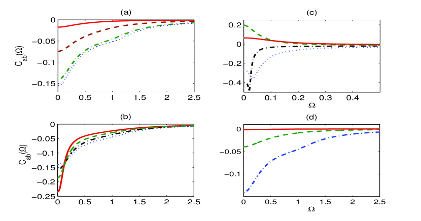
Figure 4: (Color online) Cross-correlation function, $C_{ab}(\Omega)$, for values of system parameters close to ones given by Eq.(47). (a) Cross-correlation function for different values of pumping rate. Solid, dashed, dash-dotted and dotted lines correspond to $R_{a}=R_{b}=1.001\bar{R}_{a},1.005\bar{R}_{a},1.01\bar{R}_{a},1.011\bar{R}_{a}$; other parameters are as in Fig.3(a). (b) Cross-correlation function for larger overlaps of VECSELs active zones; solid, dashed, dash-dotted, dotted lines correspond to $\xi_{a}=\xi_{b}=0.5,0.6,0.7,0.8$; other parameters are as in Fig.3(b) (c) Cross-correlation function for smaller overlaps of VECSELs active zones; solid, dashed, dash-dotted, dotted lines correspond to $\xi_{a}=\xi_{b}=0.1,0.2,0.3,0.4$, other parameters are as in the panel (b). (d) Cross-correlation function for different values of the interaction constant; solid, dashed and dash-dotted lines correspond to $g=0.01\kappa_{a},0.05\kappa_{a},0.1\kappa_{a}$; other parameters are as in Fig.2(d).

For illustration of results described by Eqs. (42-46), let us consider the simplest symmetrical situation, when both coupling, overlaps and modal decay rates are equal: $g_{a}=g_{b}\equiv g$, $\xi_{a}=\xi_{b}\equiv\xi$, $\kappa_{a}=\kappa_{b}\equiv\kappa$, $\kappa_{ap}=\kappa_{ap}=\kappa_{p}$; and assume the following realistic hierarchy of time-scales:

$$g=0.1\kappa,\quad\kappa_{p}=0.5\kappa,\quad\gamma_{2}=10\kappa,$$

$$\gamma_{c}=10^{2}\kappa,\quad\gamma_{\bot}=10^{3}\kappa.$$ (47)

Results of numerical simulation with parameters close to the ones given by Eq.(47) are given in Fig.2 for the normalized spectrum of the mode $a$, in Fig.3 for the normalized spectrum of the mode $b$, and in Fig.4 for the cross-correlation function (43).

First of all, notice that spectra of photocurrent fluctuations of output modes $a$ and $b$ are drastically different (notwithstanding the fact that for the chosen symmetric case the stationary values of modal intensities are the same). An explanation for this phenomenon can be guessed even from the toy model described in Subsection II.4: from Eq. (12) one can see that the symmetric modal superposition is subjected to nonlinearity, whereas the antisymmetric is not. So, for orthogonally polarized modes one should expect different noises. Then, it can be seen that spectral properties of fluctuations are strongly dependent on the overlap between active regions of VECSELs. It is possible to distinguish three different regimes of fluctuations in dependence on the overlap: the strong (approximately $0.5\leq\xi<1$), intermediate ($0.1\leq\xi\leq 0.5$) and weak ($\xi\leq 0.1$) overlap.

Let us start with the discussion of noise features common for all three regimes. In Fig.2(a) it is shown how the photocurrent noise of the output mode $a$ for fixed overlap is suppressed more with increase of the pumping rate. Quite significant suppression of the photocurrent noise can be reached (say, about $90\%$). However, with the used values of parameters (chosen to make the system operating as a class-A laser) one quickly comes out of the region of applicability of the approximation used to derive the system (40). This feature was commented upon in the previous Section. So, for the pumping rate exceeding the threshold value (38) only by $1.5\%$ the condition (36) is already breaking down. It is remarkable that regularity of the pump can even diminish noise reduction for the case (which is also illustrated in Fig. 2(a)). The reason for this is simple: the common pump for both coupled VECSEL systems induces rather strong partition noise. It obliterates the effect of regularity. Whereas for the coherent Poissonian pumping partition noise is not present. Also, it is worth noting that the harmful influence of regularity is more pronounced with increase of the pumping rate, since the terms describing the partition noise grow linearly with the pumping rate (see Eq.(III.2).

The photocurrent fluctuation spectrum for the mode $b$ depends on the pumping rate in the same way as it is for the mode $a$ for the fixed value of the overlap (Fig.2(b)).

Another feature common for all three regimes is dependence of the exhibited noise suppression on respective modal losses. It should be stressed out that for any significant suppression of the photocurrent noise to appear one needs having rather good cavity for their VECSELs. When one goes far away from this limit, noise reduction degrades significantly (Fig.2(d) and Fig.3(d)). For the coupling constant, $g$, just two orders of magnitude lower than the modal loss rate, $\kappa-\kappa_{p}$, any noise suppression is already absent. This result is rather expected, since strong modal loss is bound to destroy quickly interference effects leading to non-classicality (which is well-known fact for those trying to produce non-classical states with Kerr-type nonlinearity yurke ; glancy ).

Now let us discuss the dependence of photocurrent noise spectra on the overlap between regions of the active media. Fig.2(c) and Fig.3(c) show that the mechanism of photocurrent noise suppression for the case is indeed the correlated loss. In the regime of weak overlap (taking place approximately for $\xi\leq 0.1$) for both output modes suppression is absent. In this regime the system behaves as two nearly uncoupled VECSELs with coherent pumping and exhibits weak bunched noise diminishing with increase of the frequency (which is typical for the individual single-mode class-A VECSELs considered here a-class1 ; a-class2 ).

In the regime of the strong overlap (approximately $0.5\leq\xi<1$), the output mode $a$ shows much larger noise suppression than the mode $b$ (which is a manifestation of noise dependence on the modal polarization mentioned earlier). When the overlap becomes smaller, noise for the mode $a$ and $b$ behaves in the opposite way. Noise decreases for the mode $a$ and increases for the mode $b$ (see Fig.2(b) and Fig.3(b)). An increase of noise suppression for the mode $b$ continues well into the intermediate regime, $0.1\leq\xi\leq 0.5$, reaching the maximum when approximately half of the active media regions overlap. Whereas in this regime noise reduction for the mode $a$ is rather weak.

Since our non-classical noise suppression effect is produced by the interference of the emission channels of emitters arriving to the active media, i.e. by coupling of modes to the same emitters subjected to strong losses, it is naturally to expect a strong intermodal correlation arising as the result of this process (as it is pointed out by the simple model considered in Subsection II.4, where it is demonstrated how the coupling between the modes arises for this case). Due to different behavior of the photocurrent fluctuation spectra for modes $a$ and $b$ one expects having rather non-trivial cross-correlation spectrum (43). Having nearly Poissonian noise of the mode $b$ and strongly suppressed photocurrent noise of the mode $a$ in the larger overlap regime, it is quite intuitive to see anticorrelations between modes in this regime (Fig.4(a,b)). Also, it is not surprising to have these anticorrelations diminishing with decrease of the pumping rate or emitter-field interaction constants for the fixed overlap (see Fig.4(a) and (d)).

However, notice that the maximum anticorrelation for the large overlap is reached for small frequency regions where the photocurrent fluctuations spectra for both modes are actually super-Poissonian (Fig.4(a)). This is also a manifestation of the correlated loss as an interference of the emission channels for emitters arriving to the active medium. An individual emitter emits a photon either to one mode or another, and due to a large population and polarization losses the probability to have the photon re-absorbed by the emitter is very low. This process might not prevent noises of individual modes from exhibiting bunching, but it induces anticorrelations between modes.

Maximal anticorrelation is reached in the intermediate regime where the photocurrent spectrum of the mode $b$ exhibit maximal noise reduction. With further decrease of the overlap anticorrelations are eventually washed out tending to small positive correlations in the small overlap regime (Fig.4(c)). Notice that maximal increase of the anticorrelations has obviously resonant character depending strongly on the overlap and the frequency; the maximum anticorrelation is reached for the overlap corresponding approximately to all three regions $R_{j}$ being equally sized (see Fig.1).

It should be noticed that correlations between modes are even more sensitive to modal losses than non-classicality of individual modes (see Fig.4(d)). As it should be expected, modal losses into independent additional dissipative reservoir are prone to obliterate quickly the effect of the correlated loss (i.e. coupling to the same reservoir) mogilevtsev kerr 2009 . One should really be not far from the good cavity limit to have significant correlations between modes in two coupled VECSELs considered here.

VI Conclusions

In this work we have demonstrated that the system of two coupled VECSELs can indeed be a class-A laser, if it is sufficiently close to the threshold. We have developed a simple model based on the quantum Langevin equations that leads to the semiclassical equations for the intensities of two surviving orthogonally linearly polarized output modes similar to the equations describing the class-A laser. We have demonstrated that both suppression of photocurrent fluctuation noise below the standard quantum limit and strongly negative cross-correlation (anticorrelation) are possible in the system. It is remarkable that the mechanism of noise suppression arising in this case is quite different from the already well-known mechanism of inducing noise suppression through the regular pumping. In our case non-classicality arises through correlated loss, i.e. due to simultaneous coupling of both modes to the same emitter and quick decay of populations and polarization of this emitter. It is demonstrated by disappearance of non-classicality for small overlap between active regions of VECSELs, when the dynamics of each VESCEL is essentially as for an individual independent laser. For both strong and moderate overlap it is possible to reach quite strong suppression of photocurrent fluctuations (5-10 dB) and large anti-correlations. Notice, that regularity of the pumping does not enhance non-classicality available with coherent pumping. Actually, as a consequence of partition noise arising due to the pump being common for both VECSELs, regularity of the pumping can actually be harmful for non-classicality.

Appendix A Linearized equations for quantum fluctuations

Here we write down vectors of variables and non-homogeneous part of the linearized system (40):

$$\overrightarrow{X}=\begin{pmatrix}\delta a_{+}\\ \delta a_{-}\\ \delta b_{+}\\ \delta b_{-}\\ \delta a_{+}^{\dagger}\\ \delta a_{-}^{\dagger}\\ \delta b_{+}^{\dagger}\\ \delta b_{-}^{\dagger}\\ \delta P_{+}\\ \delta P_{-}\\ \delta Q_{+}\\ \delta Q_{-}\\ \delta\Xi_{+}\\ \delta\Xi_{-}\\ \delta P_{+}^{\dagger}\\ \delta P_{-}^{\dagger}\\ \delta Q_{+}^{\dagger}\\ \delta Q_{-}^{\dagger}\\ \delta\Xi_{+}^{\dagger}\\ \delta\Xi_{-}^{\dagger}\\ \delta M_{2+}\\ \delta M_{2-}\\ \delta N_{2+}\\ \delta N_{2-}\\ \delta\Lambda_{2+}\\ \delta\Lambda_{2-}\\ \end{pmatrix},\quad\overrightarrow{Z}=\begin{pmatrix}f_{a+}\\ f_{a-}\\ f_{b+}\\ f_{b-}\\ f_{a+}^{\dagger}\\ f_{a-}^{\dagger}\\ f_{b+}^{\dagger}\\ f_{b-}^{\dagger}\\ F^{P}_{+}\\ F^{P}_{-}\\ F^{Q}_{+}\\ F^{Q}_{-}\\ F^{\Xi}_{+}\\ F^{\Xi}_{-}\\ [F^{P}_{+}]^{\dagger}\\ [F^{P}_{-}]^{\dagger}\\ [F^{Q}_{+}]^{\dagger}\\ [F^{Q}_{-}]^{\dagger}\\ [F^{\Xi}_{+}]^{\dagger}\\ [F^{\Xi}_{-}]^{\dagger}\\ F^{M}_{2+}\\ F^{M}_{2-}\\ F^{N}_{2+}\\ F^{N}_{2-}\\ F^{\Lambda}_{2+}\\ F^{\Lambda}_{2-}\\ \end{pmatrix}.$$ (48)

The $26\times 26$ matrix $\mathbf{D}$ can be represented in the block form as

$$\mathbf{D}=\begin{pmatrix}D_{AA}&D_{AP}&D_{AN}\\ D_{PA}&D_{PP}&D_{PN}\\ D_{NA}&D_{NP}&D_{NN}\end{pmatrix}.$$ (49)

Non-zero elements of $8\times 8$ matrix $D_{AA}$ are

$$D_{AA}(j,j)=-\kappa_{a}\quad\mathrm{for}\quad 1\leq j\leq 4,$$

$$D_{AA}(1,2)=D_{AA}(5,6)^{\ast}=\kappa_{ap}+i\omega_{ap},$$

$$D_{AA}(j,j)=-\kappa_{b}\quad\mathrm{for}\quad 5\leq j\leq 8,$$

$$D_{AA}(3,4)=D_{AA}(7,8)^{\ast}=\kappa_{bp}+i\omega_{bp},$$

and $D_{AA}(j,k)=D_{AA}(k,j)$. The elements $8\times 6$ matrix $D_{AN}$ are zeros. Non-zero elements of the $8\times 12$ matrix $D_{AP}$ are

$$D_{AP}(j,j)=D_{AP}(j,j+5)=g_{a},\quad j=1,2,5,6$$

$$D_{AP}(j,j)=D_{AP}(j,j+2)=g_{b},\quad j=3,4,7,8.$$

Non-zero elements of the $12\times 8$ matrix $D_{PA}$ are

$$D_{PA}(j,j)=D_{PA}(j+6,j+4)=g_{a}\bar{M}_{2\pm},\quad j=1,2;$$

$$D_{PA}(j,j)=D_{PA}(j+6,j+4)=g_{b}\bar{N}_{2\pm},\quad j=3,4;$$

$$D_{PA}(j+4,j)=D_{PA}(j+10,j+4)=g_{a}\bar{\Lambda}_{2\pm},\quad j=1,2;$$

$$D_{PA}(j+2,j)=D_{PA}(j+8,j+3)=g_{b}\bar{\Lambda}_{2\pm},\quad j=3,4;$$

where the stationary values of upper-level populations are given by Eq.(39). Non-zero elements of the $12\times 12$ matrix $D_{PP}$ are diagonal: $D_{PP}(j,j)=[D_{PP}(j+4,j+4)]^{\ast}=-\gamma_{\bot}-i\nu$ for $1\leq j\leq 4$. Non-zero elements of the $12\times 6$ matrix $D_{PN}$ are

$$D_{PN}(1,1)=[D_{PN}(7,1)]^{\ast}=g_{a}\bar{a}_{+},$$

$$D_{PN}(2,2)=[D_{PN}(8,2)]^{\ast}=g_{a}\bar{a}_{-},$$

$$D_{PN}(3,3)=[D_{PN}(9,3)]^{\ast}=g_{b}\bar{b}_{+},$$

$$D_{PN}(4,4)=[D_{PN}(10,4)]^{\ast}=g_{b}\bar{b}_{-},$$

$$D_{PN}(5,5)=[D_{PN}(11,5)]^{\ast}=g_{a}\bar{a}_{+}+g_{b}\bar{b}_{+},$$

$$D_{PN}(6,6)=[D_{PN}(12,6)]^{\ast}=g_{a}\bar{a}_{-}+g_{b}\bar{b}_{-},$$

where stationary modal amplitudes are taken to be real and positive (as it was pointed out in Section V), and given by Eq.(37).

Non-zero elements of the $6\times 8$ matrix $D_{NA}$ are

$$[D_{NA}(1,1)]^{\ast}=D_{NA}(1,5)=g_{a}\bar{P}_{+},$$

$$[D_{NA}(2,2)]^{\ast}=D_{NA}(2,6)=g_{a}\bar{P}_{-},$$

$$[D_{NA}(3,3)]^{\ast}=D_{NA}(3,7)=g_{b}\bar{Q}_{+},$$

$$[D_{NA}(4,4)]^{\ast}=D_{NA}(4,8)=g_{b}\bar{Q}_{-},$$

$$[D_{NA}(5,1)]^{\ast}=D_{NA}(5,5)=g_{a}\bar{\Xi}_{+},$$

$$[D_{NA}(6,3)]^{\ast}=D_{NA}(6,7)=g_{a}\bar{\Xi}_{-},$$

$$[D_{NA}(5,2)]^{\ast}=D_{NA}(5,6)=g_{b}\bar{\Xi}_{+},$$

$$[D_{NA}(6,4)]^{\ast}=D_{NA}(6,8)=g_{b}\bar{\Xi}_{-},$$

where stationary polarizations are given by Eqs.(33). Non-zero elements of the $6\times 12$ matrix $D_{NP}$ are

$$[D_{NP}(1,1)]^{\ast}=D_{NP}(1,7)=g_{a}\bar{a}_{+},$$

$$[D_{NP}(2,2)]^{\ast}=D_{NP}(2,8)=g_{a}\bar{a}_{-},$$

$$[D_{NP}(3,3)]^{\ast}=D_{NP}(3,9)=g_{b}\bar{b}_{+}$$

$$[D_{NP}(4,4)]^{\ast}=D_{NP}(4,10)=g_{b}\bar{b}_{-},$$

$$[D_{NP}(5,5)]^{\ast}=D_{NP}(5,11)=g_{a}\bar{a}_{+}+g_{b}\bar{b}_{+},$$

$$[D_{NP}(6,6)]^{\ast}=D_{NP}(6,12)=g_{a}\bar{a}_{-}+g_{b}\bar{b}_{-}.$$

Finally, non-zero elements of the $6\times 6$ matrix $D_{NN}$ are $D_{NN}(j,j)=-\gamma_{2}-\gamma_{c}$ for $j=1,2\ldots 6$; $D_{NN}(j,j+1)=\gamma_{c}$ for $j=1,3,5$; also $D_{NN}(j,k)=D_{NN}(k,j)$ for all $j,k$.

References

• (1) Y. M. Golubev and I. V. Sokolov, Sov. Phys. JETP 60, 234 (1984).
• (2) M. C. Teich, and B. E. A. Saleh, J. Opt. Soc. Am. B 2, 275 (1985).
• (3) See, for example, a classical textbook by M. Scully and M.S. Zubairy, Quantum Optics, Cambridge University Press; Chpt.14 (1997).
• (4) D. Braun, Phys. Rev. Lett. 89, 277901 (2002).
• (5) C. Horhammer and H. Buttner, Phys. Rev. A 77, 042305 (2008).
• (6) D. Mogilevtsev, Tomas Tyc, and N. Korolkova, Phys. Rev. A 79, 053832 (2009).
• (7) D. Mogilevtsev and V. S. Shchesnovich, Opt. Lett. 35 3375 (2010).
• (8) V. Pal, P. Trofimoff, B.-X. Miranda, G. Baili, M. Alouini, L. Morvan, D. Dolfi, F. Goldfarb, I. Sagnes, R. Ghosh, and F. Bretenaker, Opt. Exp. 18, 5008 (2010).
• (9) M. Fleischhauer, A. Imamoglu, and J. P. Marangos, Rev. Mod. Phys. 77, 633 (2005).
• (10) G. F. Sinclair and N. Korolkova, Phys. Rev. A 76, 033803 (2007).
• (11) F. G. S. L. Brandao, M. J. Hartmann, and M. B. Plenio, New J. Phys. 10, 043010 (2008).
• (12) G. Baili, M. Alouini, D. Dolfi, F. Bretenaker, I. Sagnes, and A. Garnache, Opt. Lett. 32, 650 (2007).
• (13) G. Baili, F. Bretenaker,M. Alouini, D. Dolfi, and I. Sagnes, J. Lightwave Tech. 26, 952 (2008).
• (14) M. San Miguel, Q. Feng, and J. V. Moloney, Phys. Rev. A 52, 1728 (1995).
• (15) J.-P. Hermier, M. I. Kolobov, I. Maurin, and E. Giacobino, Phys. Rev. A, 65, 053825 (2002).
• (16) Yu. M. Golubev, T. Yu. Golubeva, M. I. Kolobov, and E. Giacobino, Phys. Rev. A 70, 053817 (2004).
• (17) C. Benkert, M. O. Scully, J. Bergou, L. Davidovich, M. Hillery, M. Orszag, Phys. Rev. A 41, 2756 (1990).
• (18) L. Davidovich, Rev. Mod. Phys. 68, 127 (1996).
• (19) A. Bramati, V. Jost, F. Marin, and E. Giacobino, J. Mod. Opt. 44, 1929 (1997).
• (20) S. Glancy and H. M. de Vasconcelos, J. Opt. Soc. Am. B 25, 712 (2008).
• (21) M. Sondermann, M. Weinkath, and T. Ackemann, J. Mulet and S. Balle, Phys. Rev. A 68, 033822 (2003).
• (22) Yu. M. Golubev, T. Yu. Zernova, and E. Giacobino, Optics and Spectroscopy, 94, 75 (2003).
• (23) A. E. Siegman, Lasers, University Science Books, 1986.
• (24) M. J. Collett and C. W. Gardiner, Phys. Rev. A 30, 1386 (1984); C. W. Gardiner and M. J. Collett, ibid. 31, 3761 (1985); M. J. Collett and D. F. Walls, ibid. 32, 2887 (1985).
• (25) M. I. Kolobov, L. Davidovich, E. Giacobino, and C. Fabre, Phys. Rev. A 47, 1431 (1993).
• (26) B. Yurke and D. Stoler, Phys. Rev. Lett. 57, 13 (1986); Phys. Rev. A 35, 4846 (1987).
• (27) S. Glancy and H. M. de Vasconcelos, J. Opt. Soc. Am. B 25, 712 (2008).